HAL Id: cea-01484040
https://hal-cea.archives-ouvertes.fr/cea-01484040
Submitted on 6 Mar 2017
HAL is a multi-disciplinary open access
archive for the deposit and dissemination of
sci-entific research documents, whether they are
pub-lished or not. The documents may come from
teaching and research institutions in France or
abroad, or from public or private research centers.
L’archive ouverte pluridisciplinaire HAL, est
destinée au dépôt et à la diffusion de documents
scientifiques de niveau recherche, publiés ou non,
émanant des établissements d’enseignement et de
recherche français ou étrangers, des laboratoires
publics ou privés.
Magnetic critical properties and basal-plane anisotropy
of Sr 2 IrO 4
L Fruchter, D. Colson, V Brouet
To cite this version:
L Fruchter, D. Colson, V Brouet. Magnetic critical properties and basal-plane anisotropy of Sr
2 IrO 4. Journal of Physics: Condensed Matter, IOP Publishing, 2016, 28 (12),
�10.1088/0953-8984/28/12/126003�. �cea-01484040�
arXiv:1512.04448v1 [cond-mat.str-el] 14 Dec 2015
Magnetic critical properties and basal-plane anisotropy of Sr
2IrO
4L. Fruchter, D. Colson, V. Brouet
Laboratoire de Physique des Solides, C.N.R.S. UMR 8502, Universit´e Paris-Sud, 91405 Orsay, France and
+Service de Physique de l’Etat Condens´e, CEA-Saclay, 91191 Gif-sur-Yvette, France
(Dated: Received: date / Revised version: date)
The anisotropic magnetic properties of Sr2IrO4 are investigated, using longitudinal and torque
magnetometry. The critical scaling across Tc of the longitudinal magnetization is the one expected
for the 2D XY universality class. Modeling the torque for a magnetic field in the basal-plane, and taking into account all in-plane and out-of-plane magnetic couplings, we derive the effective 4-fold anisotropy K4 ≈1 10
5
erg mole−1. Although larger than for the cuprates, it is found too small
to account for a significant departure from the isotropic 2D XY model. The in-plane torque also allows us to put an upper bound for the anisotropy of a field-induced shift of the antiferromagnetic ordering temperature.
PACS numbers: 71.70.Ej,75.30.Kz,75.47.Lx,75.30.Gw
Introduction
The Ruddlesden-Popper series, Rn+1IrnO3n+1 where
R= Sr, Ba and n = 1,2,∞, has emerged as a new play-ground for the study of electron correlation effects. In these compounds, while extended 5d orbitals tend to re-duce the electron-electron interaction, as compared to the 3d transition metal compounds as cuprates, the strong spin orbit coupling (SOC) associated to the heavy Ir and the on-site Coulomb interaction compete with electronic bandwidth to restore such correlations[1]. Sr2IrO4, a
per-ovskite where a IrO2layer alternates with two SrO layer,
is structurally similar to the first discovered cuprate su-perconductor, (La,Ba)2CuO4. It was early proposed that
the strong SOC allows for an effective localized state, en-tangling spin and orbital degrees of freedom, with total angular momentum Jef f = 1/2. This spin-orbital
insu-lating state was proposed to be the analog of the Mott insulating state found in cuprates[1].
Sr2IrO4 orders antiferromagnetically below Tc ≃
240 K[2, 3]: the moments lay in the IrO2 plane and,
as the loss of the inversion symmetry in the non cubic structure – due to a rotation of the oxygen octahedra – allows for a Dzyaloshinskii-Moriya interaction, a canting of the spins (≈ 9 deg.) and a ferromagnetic component occur[4, 5] (Fig. 5). The in-plane net moments are cou-pled in an ’up-up-down-down’ way from plane to plane in zero field, and align ferromagnetically with an in-plane field H ≈ 0.2 T [6]. The initial proposition in Ref. [5] that the pseudospin Hamiltonian may be mapped onto a simple Heisenberg Hamiltonian for a square lattice anti-ferromagnet received several supports [7–10]. Recently, however, critical magnetic fluctuations were investigated using X-ray resonant magnetic scattering above Tc, and
were found consistent with the 2D XY model rather than with the isotropic model. Moreover, it was proposed that the basal-plane anisotropy accounts for the deviation of the critical exponent of the coherence length from the one of this model[11].
The magnetic ordering of a layered compound as Sr2IrO4relies, however, on the finite transverse coupling
between 2D fluctuating spins, and one cannot disregard the 3D nature of this coupling, when the ordered state is considered. So, it is necessary to also investigate the dimensionality of the fluctuations as the ordering tem-perature is crossed. The critical scaling of the magneti-zation allows to do so, as shown in section I. Besides these conventional magnetization studies, the transverse mag-netization provided by torque measurements is a direct way to evaluate the additional anisotropy in the basal-plane. Section II presents such measurements, and mod-els the system in an in-plane magnetic field to obtain an estimate of the four-fold magneto-crystalline anisotropy. It is discussed whether the measured anisotropy is able to reduce the dimensionality of the magnetic system, as proposed in Ref. 11.
I. LONGITUDINAL MAGNETIZATION
The longitudinal magnetization of a single crystal with dimensions 1200 x 400 x c = 120 µm3 was measured
in magnetic fields up to 7 T. It was grown using a self-flux technique in platinum crucibles, similar to the one in Ref. [2]. In a mean-field approach, the Weiss-molecular theory allows to predict an asymptotic linear relation-ship between the squared magnetization, M (T, H)2 and
the inverse susceptibility, H/M , in the vicinity of Tc,
which is the basis for the determination of Tc from the
so-called Arrott plot, which displays M2 vs (H/M )[12].
Below Tc, such a plot may be linearly extrapolated to
the positive saturation magnetization, Ms, while, above
Tc, the isotherms extrapolate to negative values and
in-tercept the (H/M ) axis at the inverse susceptibility χ−10 ; the isotherm at T = Tc is the one extrapolating to the
origin.
In the general case where the mean-field approach fails, a modified Arrott plot must be built, which incorporates the general scaling relations for the magnetization and susceptibility at Tc:
2 0 1 2 3 4 0 2 4 β = 0.24 γ = 0.92 246 K 216 K 1 0 - 3 M 1 / β ( e m u c m - 3 ) 1 / β 10- 4 ( H / M )1 / γ ( Oe cm- 3 emu- 1 )1 / γ a) 215 220 225 230 235 240 0 b) T ( K ) MS β ( a .u .) 0 χ 0 - γ 0.1 0.2 0.3 1E-6 1E-4 0.01 1 β
FIG. 1: (a) Modified Arrott plot for magnetic field applied along a/b axis. The inset displays the distance between the seed (β,γ) of the procedure and its output. (b) Asymptotic spontaneaous magnetization (MS) and initial inverse
suscep-tibility (χ−1
0 ) as obtained from (a). Lines are best linear fits
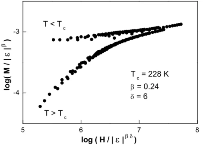
of Mβ s and (χ−10 ) γ. 5 6 7 8 -4 -3 T > T c T < T c T c = 228 K β = 0.24 δ = 6 lo g ( M / | ε | β ) log ( H / | ε |β δ)
FIG. 2: A scaling plot for M (H), using β as found in Fig. 1b.
The mean-field result is retrieved, taking β = 1/2 and γ = 1. In practice, the appropriate exponents are rarely easily obtained in this way, as the isotherms may be only asymptotically linear, and several sets of β and γ val-ues may provide equally satisfying plots (see for instance Ref. 13). So, an unbiased procedure is desirable, and we achieved this in the following way.
From magnetization isotherms obtained in the interval 216 K < T < 246 K and 0.5 T < H < 7 T, we have built the modified Arrott plot for a grid of β and γ values. For each of these plots, we have first determined the critical isotherm (as the one closest to a line crossing the origin); obtained the extrapolated values for Msand χ−10 (as the
isotherms are not completely saturated at the maximum field in Fig. 1, we have assumed that they exponentially reach the critical isotherm slope), and finally computed the β and γ values from power law fits of these quantities (as in Fig. 1b). The self-consistent plot, for which the computed β and γ values were closest to the initial seed (the distance between the seed of the procedure and its output is shown in the inset of Fig. 1a), is obtained for β = 0.24 ± 0.02, γ = 0.92 ± 0.1, and Tc = 228 ± 1 K.
Another way to obtain the scaling exponents is to use the reduced equation of states:
M/ |ǫ|β = f±(H/Mβδ) (2)
where f± refer to data for T > Tc and T < Tc
re-spectively, and ǫ is the reduced temperature. Using the previous values for β and Tc, the best scaling is obtained
for δ ≃ 6 (Fig. 2). This is compatible with the Widom scaling relation, δ = 1 + γ/β = 5.2 ± 0.9.
Away from the critical region, the data is well de-scribed by the conventional Curie-Weiss law, using TCW
= 252 ± 2 K. As seen in Fig. 3, the Curie-Weiss law breakdowns at a temperature T∗ ≃ 275 K. This is
the temperature at which an atomistic description fails. We may estimate the Levanyuk-Ginzburg criterion from the temperature range of these critical fluctuations as tG ≃ (Tc− T∗)/Tc ≃ 0.2. Using the expression in 2D,
tG= ∆Cp−1χ−20 , and Cp≃ 4mJ/mole K (Ref. 14), yields
ξ0/a ≃ 102 for the zero-temperature coherence length.
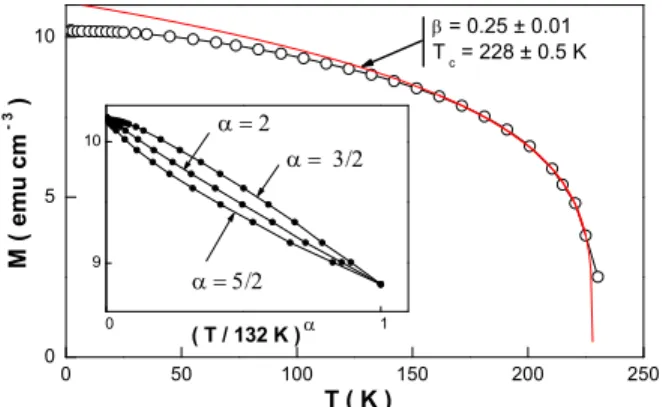
Remarkably, the applied magnetic field does not seem to change the dimensionality of the critical fluctuations to-wards a 1D behavior, as is often observed (see Ref. [15] for a review). This is also evidenced by low field mag-netization as in Fig. 4, for which a power-law fit yields β = 0.25 ± 0.01, in agreement with the high-field scaling analysis. Surprisingly, the scaling for T → 0 indicates neither a spin 1/2, 2D (T3/2), nor a 2D anisotropic or
1D universal behavior (T5/2), but clearly a 3D one (T2
-Fig. 4). This could be an indication that the transverse coupling cannot be neglected in the weakly fluctuating regime.
These results indicate clearly that the magnetic transi-tion is dominated by critical fluctuatransi-tions, which are not in the mean-field universality class. The value found for β is compatible with the 2D XY model (β = 0.23), but are hardly compatible with a strong in-plane anisotropy, for which the exponent is pushed toward the one of the 2D Ising model (β = 0.125), as discussed in Ref. 11. In the following, we investigate the in-plane anisotropic proper-ties, using torque magnetometry.
II. TORQUE MEASUREMENTS A. Experimental results
Torque magnetometry essentially measures the magne-tization component transverse to the applied field, being Γ = M × B. Thus, for a magnetic field applied in the easy a-b plane, it senses the deviation of the magneti-zation direction from the applied field one, as a result of the basal-plane magnetocrystalline anisotropy, which tends to align the spins with specific directions.
Torque was measured using a home-made setup, built from AFM piezolevers[17]. This very sensitive device cannot accommodate large samples, and a smaller crys-tal was used, selected from the same batch as for the
250 300 350 400 0 1 2 3 T c T* = 275 K T CW = 252 K m 1 (m o le e m u 1 ) T ( K )
FIG. 3: Curie-Weiss law, defining TCW and T∗(H = 0.2 T).
0 50 100 150 200 250 0 5 10 β = 0.25 ± 0.01 T c = 228 ± 0.5 K M ( e m u c m 3 ) T ( K ) α = 3/2 α = 5/2 α = 2 ( T / 132 K )α 0 1 9 10
FIG. 4: Low field magnetization data (H = 0.4 T). The line is the best fit to a power-law (Tc−T )β for T > 162K. The inset shows that M (T → 0) is best described by the 3D spin 1/2 scaling, T2
(a small Curie term is present – ≈ 0.4% at 1 K – which was not removed).
crystal used for conventional magnetometry. This par-allepipedic sample (240 x 240 x c = 100 µm3) had a T
c
identical to the one of the larger crystal, and we could also check that its anisotropic magnetic properties (char-acterized by the characteristic field H2– see below) were
also identical. Torque measurement were performed by rotating the magnetic field in the a-b plane, in magnetic fields up to 9 T. Torque signals showed a small two-fold component – typically 10% of the four-fold component – which we assign to a small misalignment of the rota-tion plane from the a-b one, so that torque also picks up part of the axial strong anisotropy. This component was systematically subtracted from the torque data as a function of the magnetic field angle, as was done for the one displayed in Fig. 6. The torque per unit volume due to the demagnetizing field may be estimated as:
Γdemag≈ 2M2∆N sin(4θ) (3)
where M is the magnetization and ∆N is the demag-netizing factor variation when the magnetic field is
ro-FIG. 5: Left: conventions used for torque measurements. Right: two adjacent IrO2 layers, antiferromagnetically
cou-pled (torque is positive for the upper layer - open arrow is the net magnetization in each layer).
0 45 90 -10 -5 0 5 10 a) H = 800 Oe Γ ( N m -2 ) θ ( deg. ) 0 45 90 -10 -5 0 5 10 Γ ( N m -2) b) H = 1000 Oe θ ( deg. ) 0 45 90 -4 -2 0 2 4 Γ ( N m -2) c) H = 1500 Oe θ ( deg. ) 0 45 90 -10 0 10 Γ ( N m -2) d) H = 2.5 10 4 Oe θ ( deg. )
FIG. 6: Torque for T = 215 K. Circles are for increasing θ; crosses, for decreasing ones. Note the difference in the torque scale. Conventions for θ and Γ are displayed in Fig. 5.
tated in the plane. Using either the approximation of an ellipsoid, or the demagnetizing factor computed for a square-shaped sample[18], we obtain ∆N ≃ 6 10−2.
Using typical value for the magnetization (e.g. M ≃ 8 emu cm−3 in the ordered state or χ ≃ 1 emu cm−3 in
the paramagnetic state at 280 K), we obtain Γdemag ≃
10−2 - 10−1 Nm−2, which is negligible, compared to the
torque signal discussed in the rest.
As expected from the quadratic symmetry of the crys-tal, the torque signal has a four-fold periodicity. Above some critical field H2 ≃ 103 Oe, the signal is to a very
good approximation sinusoidal (Fig. 6c,d), while, below this field, it shows a typical metastable behavior at θ = π/4 (Fig. 6a, b). Remarkably, the amplitude of the signal is not monotonous with the applied field, and a drop by about 50% is observed at the crossing of H2.
A systematic study of the torque signal at a fixed angle confirms this feature, and allows to uncover some others.
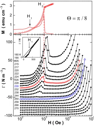
4 Figure 7 shows the torque signal obtained for θ = π/8 for
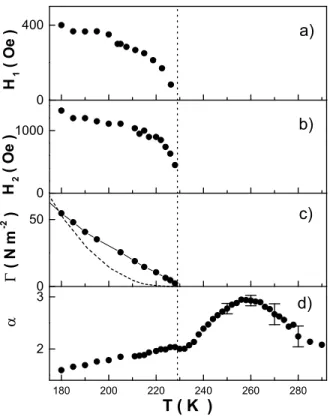
several temperatures, as well as the longitudinal magne-tization at a selected temperature T = 220 K. A sharp drop of the signal is observed at H2(T ), also displayed in
Fig. 8b. This coincides with the maximum slope of the longitudinal magnetization, m(H) (Fig. 7, upper panel). A much weaker feature is also present at a smaller field, H1(T ). Upon crossing this field, the longitudinal
mag-netization shows a small step (as evidenced by dm/dH in the upper panel in Fig. 7), and so does the transverse magnetization (Fig. 7, inset in the lower panel). Both characteristic fields H1(T ) and H2(T ) sharply drop to
zero at Tc (Fig. 8).
For fields larger than H2(T ), the torque signal shows
a plateau where it is roughly independent of the applied field (this is most evident a few K from Tc, where the
plateau is visible over a magnetic field decade). At still larger magnetic field, a noticeable increase of the torque signal occurs. It could be well fitted using a simple power law, Hα, which we found could be valid over one field
decade (the limitation being the maximum torque which our device could stand). Fitting the torque signal with such a power law, superimposed to a constant offset, yields the value of the plateau, as well as the exponent and the magnitude of the high field signal. It is found that the field-independent signal decreases to zero at Tc,
in a quasi-linear way (Fig. 8c), while the high field expo-nent varies between α ≃ 1 at low temperature and α ≃ 3 at 260 K (Fig. 8d).
B. Zero temperature model
Clearly, the interpretation of the anisotropic magnetic properties of Sr2IrO4 is made difficult by the complex
magnetic interactions hosted by this material. In the following, we introduce these interactions one after the other, in order to gauge the importance of the different contributions, and finally elaborate a model accounting for the observations.
First, we neglect the interlayer coupling and thus con-sider each layer separately. In this case, the magnetic configuration is essentially the one of a 2D antiferromag-net, with a four-fold anisotropy reflecting the quadratic symmetry of the crystal, with the additional feature of an in-plane ferromagnetic component (Fig. 5). The torque for an anisotropic 2D antiferromagnet in an in-plane mag-netic field was computed in ref. 19 and applied to the case of the cuprate Bi2CuO4. Essentially, the torque
signal reflects the occurrence of a critical field, above which the AF domains flop to a configuration almost per-pendicular to the applied field, which is well known as the spin-flop transition. Above this field, the AF do-mains nearly rigidly follow the applied magnetic field and the torque signal Γ(θ) is sinusoidal, with an am-plitude independent of the applied field, 4 K4, where K4
is the in-plane anisotropy constant in a phenomenologi-cal representation[19]. Identifying the intermediate-field
102 103 104 105 -100 -50 0 50 100 180 K 190 205 215 217 220 222 224 226 228 230 232 238 244 250 258 266 270 Γ ( N m 2 ) H ( Oe ) 0 1 2 3 M ( e m u c m 3 )
Θ = π / 8
0 500 0 H 1 Γ / H H 2 H 1FIG. 7: Upper: longitudinal magnetization (T = 220 K) and it derivative, dM/dH. Lower: torque (curves have been shifted for clarity). The inset in the lower panel displays the transverse magnetization, Γ/H, at T = 215 K, and triangles are for T = 230 K.
torque plateau in Fig. 7 with this regime, the torque value in Fig. 8c is then simply 4 K4sin(4θ). This
al-lows to estimate K4 = 8 103 erg mol−1 at T = 180 K.
It is then possible to estimate the spin-flop critical field,
Hf lop = (16 K/ χ⊥)1/2, where χ⊥ is the magnetic
sus-ceptibility for a magnetic field perpendicular to the spin-axis, and where we have neglected the susceptibility in the spin direction. Using the measured linear part of the magnetization m(H) at H = 7 T, we estimate χ⊥= 6.5
10−4emu mole−1and, neglecting χ
k, Hf lop= 2 T at T =
180 K. This is well above any of the characteristic fields evidenced by torque or longitudinal magnetization.
Actually, the ferromagnetic component must be con-sidered, as the driving torque on this component is larger than the one originating from the anisotropy of the sus-ceptibility. Neglecting the anisotropic susceptibility con-tribution, it is easy to show that the critical field now is:
Hf lop≃ 4.3K4/ ms, where msis the in-plane
magnetiza-tion. Using the measured value ms = 470 emu mole−1,
one obtains Hf lop = 160 Oe at T = 180 K. While this
value can account for the lower field H1, the model
can-not account for the second field, H2, as, for fields larger
than H1, one merely expects a rigid rotation of the layers.
To account for this second field, one needs to introduce the AF coupling between layers. The simplest model to
0 1000 H 2 ( O e ) 0 50
c)
Γ ( N m -2 ) 180 200 220 240 260 280 2 3d)
T ( K )
α 0 400b)
a)
H 1 ( O e )FIG. 8: Quantities extracted from the data in Fig. 7. a) First critical field, as given by both a step in the transverse and in the longitudinal magnetization. b) Field at the torque peak. c) Torque magnitude for H = 0.4 T. The dotted line is m(T )10
for the same field. d) Exponent for torque field dependence at high field, Γ ∝ Hα.
do so is to introduce the ferromagnetic components in two adjacent layers, and a phenomenological expression for the magnetic total energy as the sum of two terms:
Fs=
X
l=1,2
−K4cos(4 arccos(ml· a)) − ml· B
Fi= J⊥m1· m2 (4)
where the sum is for two adjacent layers, l = 1 and l = 2; mlis the ferromagnetic component in layer l, Fs
con-tains the magnetocrystalline and Zeeman energies, and Fi is for the antiferromagnetic coupling of the two
lay-ers. Although this model applies to two distinct layers, it is essentially the same as the one in Ref. 19 (using χ⊥ ∼ 1/J), with the difference that – as the magnetic
field may now reach values corresponding to the flip of the AF-coupled magnetizations – one cannot longer treat these within the anisotropic susceptibility approximation . As a result, one expects from Eq. 4 a critical field for the flop of the ferromagnetic domains similar to the one esti-mated above, which accounts for H1, and a critical field
for the flip of the AF-coupled magnetizations towards the parallel configuration, which accounts for H2. Thus, this
model offers a possibility to estimate two credible criti-cal fields, but it still cannot account completely for the
0 0.01 0.02 0
Γ
,
M
H
M Γ 0 0.02 0 3π/8 H ( a , M ) ( r a d . )FIG. 9: Torque and longitudinal magnetization, as obtained from the model of Eqs. 5. The inset displays the angle of the magnetization in the two layers, from the a-axis. Parameters for the simulation are J = 1, S = 1, K4 = 6 10−5, J⊥ = 6
10−4 and D = 0.1. The magnetic field is applied at θ = π/8.
observed torque signal. In particular, it only predicts a saturation of the torque at H2, in place of the observed
non-monotonic behavior.
We found that a realistic model may only be obtained by taking into account both the spin in-plane degrees of freedom, as for the first model, and the out-of-plane coupling, as for the second one. The total energy is then the sum of three terms:
Fs=
X
l=1,2 i=1,2
−K4cos(4 arccos(Sil· a)) − Sil· B
Fa=
X
l=1,2
J S1l · S2l − D S1l ∧ S2l
Fi= J⊥(S11+ Sl2) · (S12+ S22) (5)
where l = 1, 2 is for the two coupled layers; i = 1, 2 is for the two spins of one pair; J is the antiferromag-netic coupling of two spins belonging to the same plane; D is the Dzyalochinskii-Morya coefficient (which drives the tilt of the spins, and so generates the ferromagnetic in-plane component ml as in Eqs. 4), and J⊥
antifer-romagnetically couples m1 and m2. Strictly, the first
term should be −K4cos(4(arccos(Sil · a)) − α), where
α ≃ D/2J, to account for the octahedra rotation, but this is irrelevant for the present simulations.
As may be seen in Fig. 9, the model reproduces the essential experimental features for both the longitudinal magnetization and the torque. It is seen that, below H1, two domain orientations coexist while, above H2, the
magnetizations in the two adjacent layers are ordered fer-romagnetically and progressively rotate towards the mag-netic field orientation, as the field is increased. The peak in the torque magnitude does not mark a transition de-limiting two distinct spin configurations, but a crossover where the spin canting is found to vary by about 10%. While the only true transition at H1 produces a well
6 marked jump in the torque and magnetization
simula-tion, we have seen (Fig. 7) that the experimental mani-festation is actually weak. This may be explained both by a spatial distribution of the material properties, and by the fact that the simulation postulates identical pop-ulations of the two domain orientation below H1, and a
single stable domain above this field, while pinning and inhmogenities may well smear out the singularity.
C. Basal-plane anisotropy
Within the modelization made above, the observation, below Tc, of a torque signal increasing with field at large
field should be interpreted as the manifestation of a field-dependent parameter K4. Van Vleck first laid the basis
for a quantum theory for the computation of the magne-tocrystalline anisotropy in ferromagnetic materials[20]. He showed that the anisotropy parameter may be eval-uated using an effective anisotropic spin-Hamiltonian in the local Weiss field approximation (as a result of crys-tal field splitting and spin-orbit coupling), and the sta-tistical computation of the spin orientation distribution derived from this Hamiltonian. This distribution also determines the magnetization, and, thus, the anisotropy may be expressed as a function of this measurable quan-tity (see Ref. [21] for a review). At low temperature, when spin-waves do not destroy the two-spin correlation, this yields the well-known power law dependence, κl ∝
Ml(l+1)/2, where κ
l are the coefficients of the magnetic
energy in a spherical harmonics representation[22]. The effective anisotropy is then proportional to one of these coefficients, or a linear combination of them. This rela-tionship does not depend on the details of the spin inter-actions, but only on the symmetry of the crystal, and the order of the anisotropy. It was shown that the mean-field approximation is actually an example of a renormalized collective excitation theory, to which also belongs the spin-wave theory[23]. In this hypothesis that the spin excitations are quasi-independent, the two limiting be-haviors κl∝ Ml(l+1)/2 and κl∝ Ml, respectively in the
ordered and the paramagnetic states, are predicted. In the case of the tetragonal symmetry, the correspondence between these coefficients and the basal plane four-fold anisotropy constant is straightforward, as K4∝ κ4.
The interpretation of the power law field dependence for K4 then follows for each temperature regime. At low
temperature, M (H) is the sum of the field-independent Msand a small linear field term, so that any power law
of the magnetization yields α ≃ 1. Indeed, α decreases steadily with decreasing temperature in Fig. 8d, reaching α = 1.4 at T = 150 K. At Tc, the critical scaling gives
M ∝ Hβ/(β+γ)≃0.2(Section I), so that K
4∝ M10∝ H2,
as observed. Finally, in the paramagnetic regime, one expects K4 ∝ M4 ∝ H4. While the measured
expo-nent grows up to α ≃ 3 at T = 260 K, it is however seen to decrease for larger temperature, down to α ≃ 2. This could be due to the fact that the contribution of
the anisotropy becomes quickly smaller for higher tem-perature (as M (T )4), and the torque signal eventually
becomes dominated by some anisotropic contribution of the form ∆χH2 (i.e. ∝ M2). It is found, however,
that M (T )10 at low magnetic field does not account for
the quasi-linear temperature dependence for K4(T ) when
T → Tc(Fig. 8c). This discrepancy could sign the
break-down of the two-spins correlations by thermal spin-waves, when kBT becomes larger than the typical spin-wave
en-ergy for wave vector k ≃ a−1. Still, we evaluate the zero
temperature anisotropy from the extrapolation of K4 at
150 K to K4(0) = 1.2 105 erg mole−1, using the M10
scaling. This value is one order of magnitude larger than the one of Bi2CuO4, which should be representative of
tetragonal cuprates[19].
In Ref. 11, it was proposed that the anisotropy is large enough to influence the universality class of the fluctua-tions. In a classical description, it is not expected to do so, as long as the four-fold contribution to the free energy is smaller than the spin coupling energy, J. More pre-cisely, Ref. 24 determines K4/J ≃ 0.5. The anisotropy
energy, ≈ 0.13 µeV/spin, is only about 10−6J. The
ob-servation was made, however, that 2D quantum confine-ment yields a larger effective anisotropy for planar anti-ferromagnets, as a small anisotropy term opens a large magnon gap on the scale of J[11]. It was proposed that the effective anisotropy is in this case (24K4J)1/2 ≃ 6
10−3J. This modified value is smaller than the upper
bound obtained from the magnon dispersion in Ref. 11, 8 10−2J; it is also too small to expect a noticeable
devi-ation from the isotropic 2D XY model.
Finally, we show that torque measurements also pro-vide a way to bound possible anisotropic thermodynamic effects. In a previous contribution, we proposed that an increase of the ordering temperature with field could be at the origin of the observation of magnetoresistance effects above Tc[16]. In particular, we recalled that
the Dzyalochinskii-Morya term is the origin of a field-induced, transverse, staggered magnetic field (H†), and,
so, of a transverse staggered magnetization. This stag-gered field competes with the conventional suppression of Tc with field and, at low field, may increase the ordering
temperature in a linear way[25]. The simplest hypothe-sis to evaluate this effect above Tc is to assume a shift
of the Curie-Weiss temperature, as it should most di-rectly reflect the change in the local spin-coupling with the induced staggered field. The shift due to the stag-gered field may be estimated as ∆TCW/TCW = H†µ/J,
where H† = z hM i D/µ2, z = 4 is the coordination of the magnetic lattice, hM i the average magnetization per spin at T ≈ TCW, and µ the moment of the Ir atom.
H−1∆T
CW/TCW may be evaluated in this way as large
as 3 10−3 T−1. The anisotropic part of this shift is
how-ever not known (it was erroneously assumed that there should be one in Ref. [16], but the absence of a pro-jection of the Dzyalochinskii-Morya vector on the basal plane does not allow for this direct source of anisotropy, in the present case, unlike for La2CuO4). Assuming a
four-fold variation TCW = ∆4TCWsin(4θ), the
associ-ated contribution to torque is 4BM ∆4TCW/(T − TCW).
Using the torque amplitude measured at 260 K and 6 T as the maximum contribution for this effect, we obtain H−1∆
4TCW/TCW < 10−5T−1. So, the anisotropy of the
ordering temperature shift must be very small, if any.
Conclusion
To summarize, we have shown that the bulk magneti-zation critical scaling across Tc is close to the one
ex-pected for 2D XY scaling, as was found earlier from the temperature dependence of the magnetic coherence length, above Tc. There is no observable effect of an
in-plane magnetic field on the fluctuations dimensionality, and the scaling as T → 0 indicates the possible
impor-tance of three-dimensional fluctuations in this limit. We have modeled the longitudinal and transverse magnetiza-tions, taking into account the basal-plane couplings and anisotropy, as well as the transverse coupling. We find that the basal-plane anisotropy is too small to account for large deviations from an isotropic 2D XY model, using a simple estimate for the effective anisotropy enhancement from quantum fluctuations effects.
L.F. performed the experiments and wrote the paper, with inputs from co-authors, who also provided samples. We acknowledge support from the Agence Nationale de la Recherche grant SOCRATE.
[1] B. J. Kim, Hosub Jin, S. J. Moon, J.-Y. Kim, B.-G. Park, C. S. Leem, Jaejun Yu, T.W. Noh, C. Kim, S.-J. Oh, J.-H. Park, V. Durairaj, G. Cao, and E. Rotenberg, Phys. Rev. Lett. 101 (2008) 076402 .
[2] B. J. Kim, H. Ohsumi, T. Komesu, S. Sakai, T. Morita, H. Takagi and T. Arima, Science 323 (2009) 1329. [3] Feng Ye, Songxue Chi, Bryan C. Chakoumakos, Jaime
A. Fernandez-Baca, Tongfei Qi, and G. Cao, Phys. Rev. B 87 (2013) 140406(R).
[4] M. K. Crawford, M. A. Subramanian, R. L. Harlow, J. A. Fernandez-Baca, Z. R. Wang, and D. C. Johnston, Phys. Rev. B 49 (1994) 9198.
[5] G. Jackeli and G. Khaliullin, Phys. Rev. Lett. 102 (2009) 017205 .
[6] G. Cao, J. Bolivar, S. McCall, J. E. Crow, and R. P. Guertin, Phys. Rev. B 57 (1998) R11039(R).
[7] Vamshi M. Katukuri, Hermann Stoll, Jeroen van den Brink, and Liviu Hozoi, Phys. Rev. B 85 (2012) 220402(R).
[8] Jungho Kim, D. Casa, M. H. Upton, T. Gog, Young-June Kim, J. F. Mitchell, M. van Veenendaal, M. Daghofer, J. van den Brink, G. Khaliullin, and B. J. Kim, Phys. Rev. Lett. 108, 177003 (2012).
[9] S. Boseggia, R. Springell, H. C. Walker, H. M. Rn-now, Ch. Ruegg, H. Okabe, M. Isobe, R. S. Perry, S. P. Collins, and D. F. McMorrow, Phys. rev. Lett. 110, 117207 (2013).
[10] S. Fujiyama, H. Ohsumi, T. Komesu, J. Matsuno, B. J. Kim, M. Takata, T. Arima, and H. Takagi, Phys. Rev. Lett. 108 (2012) 247212.
[11] J. G. Vale, S. Boseggia, H. C. Walker, R. Springell, Z.
Feng, E. C. Hunter, R. S. Perry, D. Prabhakaran, A. T. Boothroyd, S. P. Collins, H. M. R¨onnow, and D. F. McMorrow, Phys. Rev. B 92, 020406(R), 2015.
[12] A. Arrott, Phys. Rev. 108, 1394 (1957).
[13] S. Zhou, K. Matsubayashi, Y. Uwatoko, C.-Q. Jin, J.-G. Cheng, J. B. Goodenough, Q. Q. Liu, T. Katsura, A. Shatskiy and E. Ito, Phys. Rev. Lett. 101, 077206 (2008). [14] S. Chikara, O. Korneta, W. P. Crummett, L. E. DeLong, P. Schlottmann, and G. Cao, Phys. Rev. B 80 (2009) 140407(R).
[15] U. K¨obler and A. Hoser, Renormalization group theory, Springer (2010).
[16] L. Fruchter, G. Collin, D. Colson and V. Brouet, Eur. Phys. J. B 88, 141 (2015).
[17] D. Zech, J. Hofer, H. Keller, C. Rossel, P. Bauer and J. Karpinski, Phys. Rev. B 53 R6026 (1996).
[18] D.-X. Chen, E. Pardo and A. Sanchez, IEEE Transac-tions on Magnetics, 41, 2077 (2005).
[19] M. Herak, M. Miljak, G. Dhalenne and A. Revcolevschi, J. Phys.: Condens. Matter 22, 026006 (2010).
[20] J. H. Van Vleck, Phys. Rev. 52, 1178 (1937).
[21] H.B. Callen and E. Callen, J. Phys. Chem. Solids, 27,1271 (1966).
[22] C. Zener, Phys. Rev. 96, 1335 (1954).
[23] H.B. Callen and S. Shtrikman, Solid State Com., 3, 5 (1965).
[24] A Taroni S T Bramwell and P C Wholdsworth, J. Phys.: Condens. Matter 20, 275233 (2008).
[25] F. Kagawa, Y. Kurosaki, K. Miyagawa and K. Kanoda, Phys. Rev. B 78, 184402 (2008).