HAL Id: cea-02890764
https://hal-cea.archives-ouvertes.fr/cea-02890764
Submitted on 6 Jul 2020
HAL is a multi-disciplinary open access
archive for the deposit and dissemination of
sci-entific research documents, whether they are
pub-lished or not. The documents may come from
teaching and research institutions in France or
abroad, or from public or private research centers.
L’archive ouverte pluridisciplinaire HAL, est
destinée au dépôt et à la diffusion de documents
scientifiques de niveau recherche, publiés ou non,
émanant des établissements d’enseignement et de
recherche français ou étrangers, des laboratoires
publics ou privés.
Distributed under a Creative Commons Attribution| 4.0 International License
Visible to near infrared multispectral images dataset for
image sensors design
Axel Clouet, Célia Viola, Jérôme Vaillant
To cite this version:
Axel Clouet, Célia Viola, Jérôme Vaillant. Visible to near infrared multispectral images dataset for
im-age sensors design. Journal of Electronic Imaging, SPIE and IS&T, In press, 106,
�10.2352/ISSN.2470-1173.2020.5.MAAP-082�. �cea-02890764�
Visible to near-infrared multispectral images dataset for image
sensors design
Axel Clouet, C ´elia Viola, J ´er ˆome Vaillant; Univ. Grenoble Alpes, CEA, LETI, DOPT, LIS, F-38000
Abstract
In this paper we present a set of multispectral images cov-ering the visible and near-infrared spectral range (400 nm to 1050 nm). This dataset intends to provide spectral reflectance im-ages containing daily life objects, usable for silicon image sensor simulations. All images were taken with our acquisition bench and a particular attention was brought to processings in order to provide calibrated reflectance data. ReDFISh (Reflectance Dataset For Image sensor Simulation) is available at: http: // dx. doi. org/ 10. 18709/ perscido. 2020. 01. ds289 .
Introduction
Spectral imaging covers all acquisition techniques producing a three dimensional datacube of the photographed scene. Outputs are described by I(x, y, λ ), where x, y are spatial dimensions and λ refers to spectral dimension. Thus each pixel of the image won’t contain luminance information as in monochrome image or RGB data as in color imaging, but a spectral information such as re-flectance of a scene. This technique is used as scientific purpose in several fields such as remote sensing, agriculture, medicine or cultural heritage. Aside these applications, reflectance multispec-tral images are also very useful for new image sensors design. It serves to simulate raw image acquisitions of realistic pictures with chosen spectral responses of the simulated sensor (and their spatial arrangement), tuned illumination and exposure conditions. Once raw acquisition is simulated, the user can also test image processings such as color correction, denoising or demosaicking. Most of image sensors produced around the world are de-signed for color application, they are usually based on CMOS technology using silicon as photodetection material. Spectrally, the silicon absorption range covers visible and a part of near-infrared (VIS-NIR) domains, between 400 nm and 1100 nm. For photography purpose, the unwanted near infrared part of the spec-trum is filtered out. However, this last part of the electromag-netic spectrum is used in various applications like de-hazing and low light imaging, or depth measurement with active illumina-tion[1]. Multispectral image dataset covering both the visible and the NIR ranges are then very useful during the development phase of such image sensors. The main motivation of the present work is to publish a new set of multispectral images to supplement the few ones already available [2][3][4] over the VIS-NIR spectrum. This paper is structured as follow: first we present the acquisi-tion setup. In the next secacquisi-tion, we detail the data acquisiacquisi-tion, im-age pre-processing and extraction of scene reflectance procedures. Then, before summarizing our work, the structure of the dataset is described including file format and some sample images.
Model and material
Image acquisition model
The setup we designed to acquire multispectral images is based on the analysis of the image acquisition model. It guided the choice of spectral filtering and hardware. In the following we assume that we take pictures of a scene that contains only objects illuminated by external illuminant (no emitted light in the pho-tographed scene). Then, for any pixel of coordinates (i, j) in the recorded image, its signal can be written:
Si, j=CV F.a 2 pix.τint 4. f#2 . Z+∞
0 I(λ ).Rx,y(λ ).T (λ ).QE(λ ).dλ +ε (1)
with CV F the conversion factor from electrons to arbitrary digital unit (in ADU /e−), apix the pixel pitch (in m), τint the
integra-tion time (in s), f# the aperture of the objective lens, I(λ ) the
illuminant spectral distribution (in photons.s−1.sr−1.m−2.m−1), Rx,y(λ ) the reflectance spectral distribution of the object, at
co-ordinates (x, y), seen by the pixel (i, j), T (λ ) the transmission of the optics, QE(λ ) the quantum efficiency of the pixel (in e−/photons) and ε the noise term (in ADU) that includes all sources (shot noise, readout noise, dark signal, etc). Obviously the integral in equation 1 is bounded as the transmittance of the optics and the quantum efficiency are non-zero only over a limited spectral range.
Many solutions were developed to perform multi- or hyper-spectral imaging, with their own advantages and drawbacks[5]. The easiest method to implement with standard components is light filtering[6, 7] in front of the camera, using narrow band fil-ters set.
Now we can rewrite the equation by splitting the transmit-tance T (λ ) in two components: the filter transmittransmit-tance itself (Tf
λc(λ )) and the transmittance of the objective placed in front of
the sensor (Tob j(λ )):
Si, j
λc=
CV F.a2pix.τint
4. f#2 . Z+∞ 0 I(λ ).Rx,y(λ ) × Tf λc(λ ).T ob j(λ ).QE(λ ).dλ + ε (2) Hardware
Our bench is schematically described in the figures 1 and 2. The main components are the illumination, the optical filters, the camera including the sensor and the objective and obviously the scene. Each element will be detailed in following subsections. Illumination
The illuminant I(λ ) must cover the whole spectrum of inter-est, 400 − 1050nm in our case. Thus, we use two outdoor light
Figure 1: Scheme of the multispectral acquisition bench
Figure 2: Overall view of our multispectral image acquisition bench: sensor and light sources (left), scene seen from sensor point of view (right)
spots that include 400W (plug power) quartz tungsten halogen (QTH) lamp with reflector, they deliver an illumination with a spectral content close to blackbody at 2900K. This spectral prop-erty is interesting for two main reasons, on one hand, its high intensity in NIR domain compensates the decrease of the quan-tum efficiency of the camera (see figure 4). On the other hand, and compared to vapor based lightning (arc lamps or fluorescent tube), it does not own spectral lines that could be a source of error when computing reflectance data from raw acquisition. Two spots are used to ensure a uniform illumination over the scene and high irradiance: spectral transmittance of filters being narrow, the input flux in the camera may be too low leading to noisy acquisitions. A warm up of 20 minutes is applied before acquiring images in order to ensure the stability of the illumination.
Spectral filtering
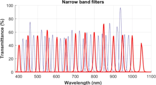
The spectral filtering is done using Thorlabs bandpass fil-ter set with a FWHM of 10nm. Central wavelengths span from 400nm to 1050nm with a step of 50nm for freely available mul-tispectral images. This first set was completed with additional wavelengths, every 20nm. Each filter was measured with a cali-brated spectrophotometer (Agilent Cary 7000) to get its transmit-tance spectrum (see figure 3).
Camera
Images are acquired using a monochrome camera DCC3240N from Thorlabs. It is based on a global shutter sensor optimized for the NIR from Teledyne-E2V (EV76C661ABT). Image contains 1280 × 1024 pixels with values coded on 10 bits. Integration time can be adjusted from 10ms to 2s. Quantum efficiency is depicted in figure 4.
To take images, a 25mm lens (Navitar MVL25M1) is mounted in front of the sensor making focus and aperture tun-able. The spectral transmittance, provided by the manufacturer is shown in figure 5.
Figure 3: Measured transmittance of filters: for freely available multispectral images in red and complementary wavelengths in blue
Figure 4: Spectral response of DCC3240N camera (from datasheet[8])
Figure 5: Spectral transmittance of MVL25M1 lens
Scene setup
The scene is placed 1.5m away from the light sources. The usable depth of the scene is limited to 15cm (all objects in the scene must be inside the depth of field of the camera). To fill the view field of the camera with objects, we built a three-step platform with black foam core cardboard being weakly reflective over the considered wavelengths range.
For reliability purpose, in each image we include the same X-Rite ColorChecker Passport Photo[9] at the bottom center part of the scene (shown later in figure 7a).
In addition, for flat-field correction, the platform is removed and we placed a white cardboard in the same plane.
Fourier analysis and sampling performance vali-dation
The sampling performance of the experimental setup can be evaluated thanks to a Fourier analysis. The goal of our acquisi-tion setup is to sample the reflectance spectrum at each pixel lo-cation of the image using the narrow band filters. To analyse the performance of the sampling setup, we can compare measuring functions to reflectance data in terms of variation spectra. For this approach, we used normalized power spectral densities computed thanks to Fourier transforms.
Thereby, we can consider that the target signals are contin-uous reflectances (denoted R) whereas each measuring function (denoted M) is given by the multiplication of the camera spec-tral response (figure 4) and respectively each narrow band filter (figure 3). In this analysis, as the illuminant is supposed to be smooth (and fixed), we do not take it in consideration. In a simple form, the sampling of reflectance data (denoted ˜R) and its corre-sponding Fourier transform can be written as in equation 3 (∗ is a convolution),F denotes the fast Fourier transform operator. So measuring function acts like a low pass filter in terms of variation frequencies, we perform a pre-study over known reflectance data to verify if the frequency content of potential target reflectances will be cut or not.
˜
Rx,y= Rx,y∗ M
F ( ˜Rx,y) =F (Rx,y).F (M)
(3) Numerous examples of reflectance data that have been ac-quired using high resolution spectrophotometers are provided by the U.S Geological Survey [10]. This spectral dataset includes various materials such as vegetations, soils, minerals, artificial materials, etc... Additionally, we measured reflectance spectra of the X-Rite ColorChecker Passport with a high resolution spec-trophotometer Agilent cary 7000 (see figure 7a).
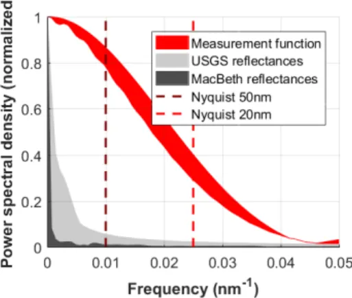
Figure 6: Bundle of normalized power spectral densities of mea-surement functions, USGS reflectances, X-Rite ColorChecker re-flectances. Nyquist frequencies are displayed for the two sam-pling steps, respectively 50 nm and 20 nm.
In figure 6, we displayed the bundle of the normalized spectral densities of measuring functions and many different re-flectance data. Frequencies of target rere-flectances are significantly lower than measuring functions ones, moreover, frequency con-tent of targets at both Nyquist frequencies are very low especially
for the X-Rite ColorChecker Passport. These results show that our acquisition setup owns good sampling properties to ensure accurate reconstruction of reflectance data.
Image acquisition and processing
In this section we detail the image acquisition procedure and the associated processings. At first, the camera is set to deliver raw uncorrected images. This is done by turning off all auto-corrections in the camera software (ThorCam): like auto-gain and gamma, dark level and bad pixel corrections, etc. As shown in equation 2, any image contains a noise parts, denoted ε. This generic term covers all sources of unwanted signal and can be split in two part: either temporal noise, or biases like dark signal. To reduce temporal noise, we averaged several images taken in the same conditions. To suppress the biases, specific images are needed: dark images, taken with the same setting than image of interest but without light, and flat field images where we capture a uniform scene. So the acquisition procedure of light image is the following:
1. For each filter, we start adjusting the integration time such that image histogram covers the 10 bits of the camera, with-out saturation.
2. Take several images of the scene, typically 4 to 10. 3. Take several dark images by placing a cap over the objective
lens, with the same settings.
This is done for each scene, but also for flat field image which are taken every day as we check that illumination unevenness remains stable.
Standard image corrections
We apply some classical corrections to get a signal value that matches with the acquisition model given in equation 1.
To summarize corrections, lets denote:
• Iλc a given raw image of interest, acquired with the narrow band filter centered at λcand with an integration time τλc
• ID,λcthe dark frame with same integration time τλc • IFF,λc the flat field frame, for which the exposure is tuned
by adjusting the integration time τFF
λc
• IDFF,λcthe dark frame with integration time τ
FF λc
Note that flat field correction is performed for all spectral filters to overcome chromatic aberrations issues. In each case, several images are taken and averaged to reduce the temporal noise. Lets denote ˆI the averaged image. The corrected image Sλc is then given equation 4.
Sλc=
ˆIλc− ˆID,λc
ˆIFF,λc− ˆIDFF,λc.max( ˆIFF,λc− ˆIDFF,λc) (4)
One must notice that flat field correction is a relative correction, as explicitly written equation 4 it is usual to normalize flat frames by there maximum intensity values.
Additionally to these different correction steps, we per-formed a post-processing alignment. In all multispectral images, landmarks have been placed (top left). We extract a ROI of 50 × 50 pixels around the mark and the potential displacement is estimated by computing the cross-correlation between the ROI
of the current frame and the ROI of a reference frame (we choose λ = 550nm as reference). The location of the maximum of the cross-correlation gives the displacement amount and the image is registred by applying the translation vector.
Reflectance extraction
To extract the reflectance values from a corrected image Sλc, we work with the equation 2. The Fourier analysis showed that reflectance spectra have smooth variation as they contain low frequencies compared to measuring function. Consequently, re-flectance can be considered to be constant over the transmittance range of a single narrow band filter. As the illuminant is consti-tuted of halogen lamps and won’t vary during the acquisitions, we suppose it varies smoothly compared to measuring function. Thus, we approximate them by their value at the central wave-length of the filter. Under this hypothesis, we can rewrite equation 2 by taking out of the integral I(λc) and Rx,y(λc):
Si, j
λc =
CV F.a2pix.Tint
4. f#2 .I(λc).Rx,y(λc) × Z+∞ 0 Tf,λc(λ ).Tlens(λ ).QE(λ ).dλ + ε (5)
However, at this point, reflectance extraction is still not ac-curate since several uncertainties are remaining. First, CVF is not precisely given by the manufacturer of the camera, despite an ex-perimental evaluation, the value remains an approximation of the real one. Then, aperture factor f# is not perfectly known since
the lens aperture setup is not notched. Moreover, spectral trans-mittance Tlens(λ ) of the lens is given by the manufacturer but it
can vary according to the aperture value or even between manu-factured lot. Next, the spectral repartition of the illuminant has not been measured precisely (lamp manufacturers only give color temperature). Finally there is a multiplying factor resulting from the flat field correction which is arbitrary based on the maximum value of each flat field frame. To compensates all these inaccura-cies, we use a pre-calibration to estimate an experimental effective illuminant we call ˆI(λc).
(a)
(b)
Figure 7: Example of reflectance spectra measured with Agilent Cary 7000 spectrophotometer on X-Rite ColorChecker Passeport (patches are surrounded with red square
To remove these uncertainties, we measured spectral re-flectance of X-Rite ColorChecker chart in a spectrophotometer
figure 7a. For each patch, we know Rx,y(λc) and we can extract
ˆ
I(λc) using equation 5. We expect to get the same evaluation of
ˆ
I(λc) for each color patch. To evaluate small modifications of this
illuminant along the time, an X-Rite ColorChekcer Passeport has been placed in all multispectral images.
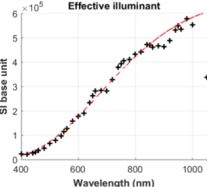
We observed negligible differences of the effective illumi-nant value from an image to another, so we used the same one for all the images. The mean of these effective illuminants is dis-played in figure 8.
Figure 8: Measured effective illuminant (black crosses), fit with a black body spectral repartition at 2970K (red dash line)
Once the effective illuminant is fixed, the reflectance of a given scene can be extracted directly from equation 5, then we can compare reflectance data from multispectral images to those mea-sured with the spectrophotometer. Figure 9 shows this compari-son for random pixels selected in the middle of the color patches in a randomly chosen image (here it is ”LeatherFace”).
Figure 9: Comparison of reflectance spectra from multispec-tral image (crosses) versus spectrophotometer measurement (solid line)
Results and dataset
We built up the dataset using the procedure described above, each multispectral image is composed of a data cube (size 1280 × 1024 × 14) containing reflectance on the third dimension. The dataset is constituted of indoor images that mainly contain com-mon life objects with different colors and textures. It is freely available as a single zip file on PerSCiDO platform: http:// dx.doi.org/10.18709/perscido.2020.01.ds289. This file contains 22 datacubes in hdf5 format (structure described below) and 22 images in png format to facilitate the image identification.
File format
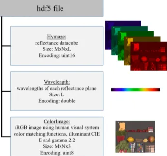
To store the reflectance datacube, the wavelength and an RGB image, we choose the hierarchical file format hdf5 [11], which can be easily read with scientific language like Python or Matlab. It simply contains 3 fields (see figure 10):
• Hymage: the reflectance data cube, size is 1280 × 1024 × 14 and is encoded on uint16, so reflectance is R = Hymage/(216− 1)
• Wavelength: the wavelength, in nm, of each plane and en-coded in double
• ColorImage: sRGB (gamma = 2.2) image, size is 1280x1024x3, generated from the reflectance data cube, hu-man visual system color matching function and CIE E illu-minant.
Figure 10: File format description
Samples
The figure below shows some of the scenes we shot: plants and flowers (11a), fruits and vegetables (11b), make-up mate-rial (11c), woods of different species (11f), tained leather patches (11d), and pastel pencils (11e).
Summary
We presented in this paper a dataset of multispectral re-flectance images covering the visible and a part of the near-infrared spectrum corresponding to the absorption range of the silicon. This set intends to supplement the already available datasets and was generated to provide useful images for sensor simulation (daily life objects). We included in all images an X-Rite ColorChecker chart for color correction implementation and we took a great care to image acquisition and pre-processing to limit the noise and uncertainties in the data. The dataset (called ReDFISh) with spectral sampling every 50nm between 400nm and 1050nm is freely available for download at http://dx.
(a) (b)
(c) (d)
(e) (f)
Figure 11: Image samples
doi.org/10.18709/perscido.2020.01.ds289, and comple-mentary data with 20nm may be available on request (contact us at e-mail address displayed in authors biography section).
Acknowledgment
The authors would like to thanks the University of Grenoble Alpes, PERSYVAL-Lab and the PerSCiDO platform for hosting the dataset. We also want to thank people in CEA-LETI who pro-vided great help and support for the bench setup. Finally, many thanks to David Alleysson and Mauro Dalla Mura for fruitful dis-cussions.
References
[1] N. Pears. 3D Imaging, Analysis and Applications. Springer, 2012.
DOI: 10.1007/978-1-4471-4063-4.
[2] M. Parmar et al. “A Database of High Dynamic Range Visible and Near-Infrared Multispectral Images”. In: Digital Photography IV. Vol. 6817. International Society for Optics and Photonics, 2008, 68170N.
[3] J. Eckhard et al. “Outdoor Scene Reflectance Measurements Us-ing a Bragg-GratUs-ing-Based Hyperspectral Imager”. In: Applied Optics54.13 (May 1, 2015), p. D15.ISSN: 0003-6935, 1539-4522.
DOI: 10.1364/AO.54.000D15.
[4] Y. Monno et al. “Single-Sensor RGB-NIR Imaging: High-Quality
Journal19.2 (Jan. 2019), pp. 497–507.ISSN: 2379-9153.DOI: 10.1109/JSEN.2018.2876774.
[5] J. Qin et al. “Hyperspectral and Multispectral Imaging for Eval-uating Food Safety and Quality”. In: Journal of Food Engineer-ing118.2 (Sept. 1, 2013), pp. 157–171.ISSN: 0260-8774.DOI: 10.1016/j.jfoodeng.2013.04.001.
[6] G. Lu et al. “Medical Hyperspectral Imaging: A Review”. In:
Journal of Biomedical Optics19.1 (Jan. 2014).ISSN: 1083-3668.
DOI: 10.1117/1.JBO.19.1.010901.
[7] D. Wu et al. “Advanced Applications of Hyperspectral Imaging
Technology for Food Quality and Safety Analysis and Assess-ment: A Review — Part I: Fundamentals”. In: Innovative Food Science & Emerging Technologies19 (July 1, 2013), pp. 1–14.
ISSN: 1466-8564.DOI: 10.1016/j.ifset.2013.04.014.
[8] Thorlabs.URL: https://www.thorlabs.de/.
[9] X-Rite.URL: https://www.xrite.com/.
[10] USGS.URL: https://www.usgs.gov/.
[11] HDF-Group.URL: https://www.hdfgroup.org/.
Author Biography
Axel Clouet received his Master degree in semi-conductors physics and photonics from Grenoble Institute of Technology -Phelma (France) in 2017. He is currently pursuing his PhD at the department of optics and photonics of the CEA-LETI of Greno-ble. His interest is now focused on signal and image processing for color and multispectral imaging.
Contact: axel.clouet@cea.fr
C´elia Viola received her Associate’s Degree from Grenoble-Alpes University Institute of Technology, France (2019).
J´erˆome Vaillant received his M. Sc. in Optical Engineer-ing from Ecole Centrale de Marseille, France (1996), his M. Sc. Degree in Astrophysics from Grenoble Alps University, France (1997) and his Ph.D. in Astrophysics from Lyon Univer-sity, France, in 2000. Since then he has worked on CMOS image sensor with a focus on optics at pixel. Starting in 2000 at STMi-croelectronics R&D center in Crolles, France, he joined CEA in Grenoble, France, in 2012.