HAL Id: hal-01852585
https://hal.inria.fr/hal-01852585
Submitted on 2 Aug 2018
HAL is a multi-disciplinary open access
archive for the deposit and dissemination of
sci-entific research documents, whether they are
pub-lished or not. The documents may come from
teaching and research institutions in France or
abroad, or from public or private research centers.
L’archive ouverte pluridisciplinaire HAL, est
destinée au dépôt et à la diffusion de documents
scientifiques de niveau recherche, publiés ou non,
émanant des établissements d’enseignement et de
recherche français ou étrangers, des laboratoires
publics ou privés.
Convolutional neural networks for disaggregated
population mapping using open data
Luciano Gervasoni, Serge Fenet, Régis Perrier, Peter Sturm
To cite this version:
Luciano Gervasoni, Serge Fenet, Régis Perrier, Peter Sturm.
Convolutional neural networks
for disaggregated population mapping using open data.
DSAA 2018 - 5th IEEE International
Conference on Data Science and Advanced Analytics, Oct 2018, Turin, Italy.
pp.594-603,
Convolutional neural networks for disaggregated
population mapping using open data
Luciano Gervasoni
∗, Serge Fenet
†, Regis Perrier
‡and Peter Sturm
§∗†§Inria Grenoble – Rhˆone-Alpes, France
∗‡§Univ Grenoble Alpes, Lab. Jean Kuntzmann, Grenoble, France ∗‡§CNRS, Lab. Jean Kuntzmann, F-38000 Grenoble, France
†Univ. Lyon 1/ LIRIS, F-69622, Lyon, France
Email:∗[email protected], †[email protected], ‡[email protected], §[email protected]
Abstract—High resolution population count data are vital for numerous applications such as urban planning, transportation model calibration, and population growth impact measurements, among others. In this work, we present and evaluate an end-to-end framework for computing disaggregated population mapping employing convolutional neural networks (CNNs). Using urban data extracted from the OpenStreetMap database, a set of urban features are generated which are used to guide population density estimates at a higher resolution.
A population density grid at a 200 by 200 meter spatial resolution is estimated, using as input gridded population data of 1 by 1 kilometer. Our approach relies solely on open data with a wide geographical coverage, ensuring replicability and potential applicability to a great number of cities in the world. Fine-grained gridded population data is used for 15 French cities in order to train and validate our model. A stand-alone city is kept out for the validation procedure. The results demonstrate that the neural network approach using massive OpenStreetMap data outperforms other approaches proposed in related works.
Index Terms—Population density, Census tract, Open data, Neural networks
I. INTRODUCTION
As often shown in the literature, numerous urban-related ac-tivities, such as business development evaluation, demographic studies, disaster prevention, and urban planning, require pop-ulation data at a fine resolution [1]–[4].
Transportation models also require population data, mainly describing both households and activities locations, in order to compute realistic origin-destination travels [5]. Indeed, the main demand for commuting nowadays is explained through residents’ daily journeys between their residence and their jobs. To this effect, population estimates at a fine resolution are of paramount importance for these models [6].
Additionally, the notion of population density exists in-trinsically in the definition of urban sprawl. Thus, capturing population densities at the neighborhood scale is of great importance to determine low-density pattern sprawling devel-opments. Nonetheless, census tract data is generally delivered at a coarse-grained low resolution. To this end, there exists a demand for methods able to disaggregate population data into a more fine-grained resolution.
The idea of using ancillary data to perform disaggregated population estimates is common to all frameworks. A com-prehensive review on disaggregated population estimates has
been carried out in [3]. In the following, we review related works according to the ancillary data employed.
Census data yields the essential data of population count, which are often available as gridded data. However, they rarely – if ever – provide a fine enough resolution for several data-demanding applications. Low temporal resolution (i.e., infrequent data collection) and low spatial resolution have been recognized as two major drawbacks of this data source [1]. Consequently, one needs to perform disaggregated mapping estimations of census tract data at higher resolutions than provided, by means of using ancillary data [7].
To help this process, LiDAR data are often used as ad-ditional topology-related data. They however remain costly to acquire, and require dedicated measurement campaigns, which remains limited to some geographical regions. Alternatively, survey data built for example from user interviews, are fre-quently used in the context of transportation models. Yet, they are expensive to obtain, and above all represents only a small percentage of the overall population.
Land Use and Land Cover (LULC) data have commonly been used as auxiliary information to carry out disaggregated population estimates at a fine resolution [8]–[10]. Generally, this type of data is inferred from satellite imagery using remote sensing techniques. Nonetheless, it has already been documented that these methods are well-suited for land-cover (i.e., physical material at the surface of the earth) estimations rather than land-use (i.e., for a same land-cover, either a residential or activity-related – commercial, industrial, shop, leisure, amenities, etc – usage) estimations [11]. This is notably relevant in those cases where a differentiation between residential and activity land uses is necessary, i.e. disaggregated population mapping. Further, information on the intensity of utilization of a land use type is not retrieved by any means, which is a crucial aspect towards computing realistic employment and residential usage estimations.
More generally, it is recognized that the application of techniques using satellite imagery is increasingly problematic with increasing population density [12]. Thus, in all likelihood, the retrieval of building heights remains highly difficult with-out the aid of complementary sources of data. This is done for instance in [2], where “building footprints and heights are first determined from aerial images, digital terrain and
surface models”. However, availability of this type of data is very limited, restricting the geographical coverage of their application.
Still, population density estimations have been carried out using satellite imagery and census data [13]. The relation between population and the area/volume of buildings has also been studied in the context of satellite imagery and with the aid of LiDAR data [1]. In this particular context, population estimation was found to be better using an area-based approach rather than a volume-area-based one. This can be explained due to the homogeneity of single-residential housing for the employed case study, and might not hold for other regions.
In [1], authors used remote-sensing-based approaches to estimate local population by: (1) identifying the number of dwelling units, (2) extracting impervious surfaces in residential areas, (3) classifying land-use types and (4) directly relating spectral reflectance to population values. A more detailed review of population estimation methods using remote sensing in the context of Geographic Information Systems (GIS) is available in [14].
It is tempting to try to learn how to infer high-resolution population data from coarser measures. Such an approach for disaggregating population data has been performed using Random forests [15]. By combining remotely-sensed and geospatial data, the method builds population density grids at the fine resolution of ∼ 100m. More recently, a method performing disaggregated population estimates at building-level (individual households) by computing residential surfaces from OpenStreetMap data has been proposed [16].
Motivation: An increasing number of sources of gridded population data are available nowadays. However, they almost never yield a very fine-grained resolution, mainly due to confidentiality reasons. This presents an inconvenience for a number of urban oriented applications, which demand a higher resolution due to their spatial expressiveness. Meanwhile, crowd-sourcing data is sharply rising, both in terms of quality and coverage. We advocate that this kind of data can be thus exploited, outperforming previous relating works in terms of population disaggregation.
Contribution: In this work we provide an end-to-end framework to perform disaggregated population mapping em-ploying a Convolutional Neural Network (CNN). To this end, a set of urban features are calculated using OpenStreetMap in order to describe the urban context, and is later employed to guide the population densities downscaling procedure. The census tract data allows to estimate the effective population count within the higher resolution grids. We rely solely on open source data, and the presented method can be applied to any region in the world as long as sufficient data exists.
Overview: Our contribution consists of 1) creating an appropriate neural network architecture to achieve our goal; 2) generating training data by means of extracting urban features for a set of cities; and 3) performing disaggregated population mapping from census tract data into a finer-grained resolution.
II. DATA
In this framework, we make use of two sources of data, providing an urban structural context and a coarse gridded population count. Both are open data, ensuring replicability of the developed framework. Additionally, the sources of data depict a world-wide coverage. Nonetheless, urban data availability still highly varies across the world.
A. Population data
Coarse grained gridded population data is necessary to provide a basis from which we compute population count estimates at a finer level. For this reason, at one point fine grained population data is needed to train our model.
Fine grained census population data is used for the country of France. The INSEE institute1 delivers the gridded data for the whole country with a resolution of 200m by 200m. This fine-grained data is used to train and validate our developed model.
Later, once the model has been trained, one can further study the applicability of the method to other countries, by leaning on other sources of data proper to each country. To this end, the Gridded Population World (GPW) dataset2 is employed,
which provides population data with a complete world-wide coverage at a resolution of ∼ 1km by 1km.
B. Urban context data
Urban structural data provides the context from which we will learn the features explaining the local variations of population, and guides the disaggregated population mapping. This urban data is extracted from the OpenStreetMap database, a prominent example of Volunteered geographic information and open data.
Volunteered geographic information (VGI) is becoming an essential source of data. Although it has been initially criticized because of potential data quality issues, the rising number of contributions made on platforms such as Open-StreetMap (OSM) have attracted the attention of researchers working on urban applications, which in addition have lead to improve its precision and completeness. VGI, and in particular in the case of open source data, are easy to access and exploit. In the specific case of OSM data, it often exhibits a better precision and completeness compared to commercial or private datasets.
A rising number of quality assessments have been proposed and carried out on OSM. [17] showed that “in many places, researchers and policymakers can rely on the completeness of OSM, or will soon be able to do so”. In several European cities, OSM footprint data (such as in Munich in the study of [18]) have a “high completeness and semantic accuracy”.
[19] showed that “For the features studied, it can be noted that change over time is sometimes due to disagreements between contributors, but in most cases the change improves the quality of the data”. OSM data have been proven to be
1https://www.insee.fr/fr/statistiques/2520034; INSEE is the French national
statistics institute.
superior compared to the official data-set for Great Britain Meridian 2 [20]. Germany’s street network is concluded to be more complete than in available commercial data-sets [21]. Similarly, Hamburg’s street network is about 99.8% complete according to the surveying office of Hamburg [22], and the volume of Points of Interest (POI) in China has increased nine-fold during the period 2007-2013 [23]. There are already more than 4 million registered users, whereas the accumulated number of contributors per month have increased to more than 1 million.
It should be pointed out that still, missing data exists for a great number of regions in the world. As a matter of trend, medium-to-big density cities tend to be more complete in terms of data, due to the number of existing contributors. As well, data availability highly varies across countries. On the one hand, some countries appear to have very few contributors, and thus urban data such as buildings have not been drawn for a great number of cities.
On the other hand, some official public institutions have started uploading their official datasets to OSM. For instance, in France the cadastral database has been uploaded3. Further,
a project4has been set up towards reaching the harmonization
of the French street addresses database – several exist but do not always match – into a single one via OSM.
Urban data availability is a key element to consider. Thus, the appropriateness of application of the present work relies upon the availability of data for the desired region of interest.
III. URBAN FEATURES PROCESSING
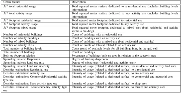
We generate a set of urban features extracted from the data and meta-data of OSM to later drive the population mapping procedure. First, we sample a regular grid at a given spatial resolution, and for each of the grid cells we compute a set of urban features or descriptors. The list of features to compute is shown in Table I. A large number of features are chosen to be extracted, given the fact that the higher the information about differing urban aspects, the better the potential to better guide the disaggregating procedure.
In order to calculate the different urban features, OSM data for an input region is requested via the Overpass API in a similar way to [24]. The OSM database consists of geometrical elements (i.e., points, lines, polygons) with associated meta-data – key-value tags – to indicate information about these elements. The following elements together with their including meta-data is retrieved:
• Buildings: using the tool provided in [24], all buildings within the region of interest are retrieved.
• Building parts: in order to reconstruct the real area asso-ciated to each building, all building parts are retrieved.
• Land use polygons: provides information about the land use within each polygon.
• Points of Interest (POI): mostly associated to activity land
uses, they allow to determine mixed-use buildings.
3https://wiki.openstreetmap.org/wiki/WikiProject France/Cadastre/Import
automatique des batiments
4http://openstreetmap.fr/bano; BANO (Base d’Adresses Nationale Ouverte)
Some building parts are filtered out if they are not necessary (“building : part”=“no” and “building : part”=“roof ”) or if the building already exists, as sometimes a tagged building contains a tag of a building part as well.
A. Classification
All the retrieved data are classified according to their corresponding land use: “activity”, “residential”, “mixed” or “other” land uses.
a) Tags information: Buildings, building parts and POIs are classified according to their input tags. We follow in this process the information provided by the OSM wiki5.
Afterwards, the land use is inferred for those buildings which do not contain this tag via the inclusion of other information, i.e. polygons with defined land use. This procedure is the same as done in [25].
b) Points of Interest: POIs in OSM are used to tag a feature occupying a particular point. Given that they are mostly associated to activity land uses, one can use them to determine the real use for several buildings. Thus, buildings containing points of interest will adopt a new class, as depicted in Table II. This procedure is motivated by the high frequency of mixed use buildings containing their activity land use in the form of a POI.
B. Land uses area calculation
a) Building levels: Data related to building height and levels are used to determine the effective number of levels per building or building part. As either the number of levels or the height of a building are frequently available, one needs to determine the equivalence between these two inputs.
This relationship between number of levels and height is computed following the assumption of a 3D visualization tool for building visualization using OSM data. Thus, it approximates the height of one level as an equivalent of 3 meters6.
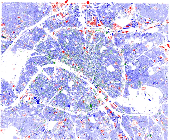
b) Area land use association: The different land use areas associated to each building are then retrieved according to the classification of the building and its inner parts. The total area associated to a building is the same as its footprint times its number of levels. In the case of mixed-use buildings, and in the absence of further information, we evenly distribute its total area to each land use (i.e. activity and residential). If a building lies at the intersection of two or more squares of the grid, the surface values are associated to each square proportionally with respect to its footprint. An example of the buildings retrieved and their land use classification is shown in Fig. 1.
Finally, we choose to include urban sprawl indices into the urban features which will later guide the disaggregated popula-tion procedure due to the fact that sprawl is directly related to the notion of population density. It is well-known that very sprawling neighborhoods or regions depict low population densities. Thus, we claim that including information about the
5http://wiki.openstreetmap.org/wiki/Map Features 6https://www.mapbox.com/blog/mapping-3d-buildings/
Fig. 1: Retrieved buildings from the OpenStreetMap database for the city of Paris, France. Buildings are classified according to their land use: residential, activity and mixed land uses depicted in blue, red and green respectively.
sprawling condition of a local neighborhood will significantly aid during the procedure of population distribution estimation. The spatial sprawling indices – land use mix, intensity of land use, and built-up dispersion – and densities estimation of different land uses are extracted making use of related works [25], [26]. Table I details the features, whereas part of them comes from the computation of sprawl measurements.
All urban features are normalized on a per-city basis, due to the feature-scaling requirement of machine learning algo-rithms. This normalization is not carried out on a global basis due to the fact that values computed within a city would in the end be sensible to the values encountered elsewhere (e.g., different cities). Thus, it is important to point out that values encountered for different urban features may vary significantly from one city to another.
The resolution used for creating the training and validation samples is guided by the input data. The gridded population data available world-wide (GPW) consists of grids of ∼ 1km by 1km. The census tract data grids available for France – used to generate the ground-truth during the supervised learning – consists of ∼ 200m by 200m.
A ground-truth sample consists thus of 25 squares of ∼ 200m by 200m, namely 5 by 5 squares, which aggregated represent the same resolution as GPW. The set of urban
fea-tures is computed for each of the squares within the finer-grid, where population count data is available. Additionally, the total population count for the complete sample is calculated, as well as the population density associated to each square.
It is to be noted that the resolution of a sample containing the 25 squares corresponds to the resolution available in the world-wide gridded population data. Nonetheless, it should be noted that they are not aligned due to the usage of different geographical coordinate systems.
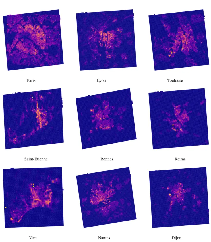
The population data used to generate the ground-truth samples – INSEE’s fine grids – for several French cities are depicted in Fig. 5. As well, several calculated urban features for the city of Paris are shown in Fig. 6.
IV. CONVOLUTIONALNEURALNETWORKS Our goal is to conceive an easy-to-use end-to-end frame-work to perform population densities downscaling using urban contextual information. Convolutional neural networks (CNN) are employed to learn a function such that population den-sities are distributed among finer grids using as input urban descriptors associated to each one of them.
CNNs consist of a stack of learned convolutional filters that are able to extract hierarchical contextual features. They represent a popular form of deep learning networks that
Urban feature Description
M2 total residential usage Total squared meter surface dedicated to a residential use (includes building levels
information)
M2 total activity usage Total squared meter surface dedicated to any activity use (includes building levels
information)
M2 footprint residential usage Total squared meter footprint dedicated to residential use
M2 footprint activity usage Total squared meter footprint dedicated to any activity use
M2 footprint mixed usage Total squared meter footprint dedicated to mixed uses (both residential and activity
within a building)
Number of residential buildings Count of buildings with a residential use Number of activity buildings Count of buildings with an activity use
Number of mixed buildings Count of buildings with a mixed-use (both residential and activity) Number of activity POIs Count of Points of Interest related to an activity use
Total number of building levels Count (sum) of available levels for all buildings lying in the grid-cell Total number of buildings Count of buildings
Built-up footprint relation Percentage of buildings built-up area in relation to the square’s area Sprawling indices: Dispersion Degree of built-up dispersion
Sprawling indices: Land use mix Degree of mixed-uses (residential and activity uses)
Sprawling indices: Land use intensity Intensity of usage (related to dedicated surface) for residential and activity land uses Densities estimation: Residential use Intensity of usage (related to dedicated surface) to a residential use
Densities estimation: Activity use Intensity of usage (related to dedicated surface) to any activity use Densities estimation: Commercial/industrial activity
type use
Intensity of usage (related to dedicated surface) to commercial and industrial uses Densities estimation: Shop activity type use Intensity of usage (related to dedicated surface) to shop uses
Densities estimation: Leisure/amenity activity type use
Intensity of usage (related to dedicated surface) to leisure and amenity uses TABLE I: Set of urban features extracted for each input square
Building
Activity Residential Mixed-use POI
Activity Activity Mixed-use Mixed-use Residential Mixed-use Residential Mixed-use Mixed-use Mixed-use Mixed-use Mixed-use TABLE II: Building’s adapted class given its own class and the classification of POIs lying inside the building.
outperform other approaches in several domains, such as digit recognition [27], natural image categorization [28], and remote sensing image analysis [29].
Convolutional layers have fewer connections and a reduced number of trainable parameters compared to fully connected layers (i.e., connected to all the outputs of the previous layer). Moreover, given the fact that the same filter is applied to each input location, translation invariance is ensured.
We favored the use of a fully convolutional architecture rather than fully connected layers for two reasons. First, it reduces the number of parameters to learn, a desirable aspect whenever vasts amount of data are not available. The complexity of a neural network can be expressed through its number of parameters, whereas the larger this number, the larger the amounts of data needed to correctly train the model. Second, the context of disaggregated population estimates urges for learning a location-invariant function. While it is possible to succeed in obtaining such a function with fully connected layers, this could end up not occurring even with vast amounts of data. For this reason we prefer to explicitly conceive an architecture which imposes restrictions on the neuronal connections.
To this end, we compute the function
f (X1, X2, ..., XN) = <Y1, Y2, ..., YN> (1)
such that Xi denotes a set of urban features associated to
grid-cell i, and Yi its estimated population density. In brief,
the function f allows to perform disaggregated population estimates into N finer grid-cells. Let P be the population count obtained from the coarse-grained input gridded data. The estimated population count for the higher-resolution cell i is directly obtained as Yi∗ P . Naturally, one needs to ensure
that
N
X
i=1
Yi = 1
The developed structure of the CNN consists of three consecutive layers, each one performing 1-dimensional con-volutions on its input. These convolutional layers contain respectively 10, 5, and 1 filter/s. As well, each of these convolutions depict a kernel size and strides of 1. Following to each layer, a ReLU activation function is employed.
Finally, after the output layer a normalized exponential function is employed, i.e. sof tmax activation function, which directly associates the estimated population densities to each grid-cell i. Thus, the sof tmax function ensures
0 ≤ Yi≤ 1 and N
X
i=1
Yi= 1
This structure yields a total number of 271 parameters. Additionally, we point out that we explicitly choose to perform 1-dimensional convolutions rather than in the 2-dimensional domain. Given the intended usage of this appli-cation, there exists an important motivation of developing a model which is as generalizable – to be applied for heteroge-neous cities – as possible, rather than being too-specific for a limited region but poorly applicable elsewhere.
Deep-learning methods are well-known for their capabilities of learning hierarchical context in order to enhance their performance. To this end, there are good reasons to believe that the application of convolutions in the 2D domain would imply including information of the neighboring urban context. Nonetheless, this would be undesirable in our particular con-text, given the fact that this type of context is specific to cities within a certain type of urban development, generally found within countries. But we argue hereby that this context can be completely different across countries, so we rather avoid including this type of contextual information in the model. Nonetheless, we shall point out that tests to confirm this hypothesis have not been carried out.
V. RESULTS We processed the following French cities:
• Rennes, Montpellier, Nice, Saint-Etienne, Bordeaux, Di-jon, Marseille, Reims, Toulouse, Paris, Nantes, Lyon, Toulon, Strasbourg, Grenoble
All of these cities sum up to a total number of 96,972 samples (i.e., each sample is represented by 25 squares of 200m by 200m with both the computed urban features and its ground-truth population density).
The neural network is trained by back-propagation using a total number of 86,904 samples. The remainder of the samples are used in the validation procedure. A stochastic gradient descent optimizer is employed with the following parameters:
• learning rate of 0.01
• learning rate decay of 1e − 6
• momentum of 0.9
• mean absolute error employed as loss function
The training procedure consists of 100 epochs using a batch size of 32 samples.
There exists no way to determine the minimum amount of samples required to effectively train a neural network. Nonetheless, a basic rule of thumb states to have at least Q2 samples to train whereas Q represents its number of
parameters. In this case Q2 = 73, 441 given Q = 271, thus the 86,904 samples minus the samples left out for validation yield enough data for the training procedure.
In the literature of population density estimation, both the root mean squared error (RMSE) and mean absolute error (MAE) are well-known and typically used accuracy measures to carry out the evaluation procedure [3], [13]. Thus, those are the chosen metrics to evaluate our proposed method.
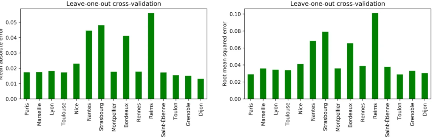
A leave-one-out cross-validation was carried out. The ob-tained mean across the mean absolute errors consists of 2.53%, whereas for the root mean squared error was computed to 4.62%. Fig. 2 shows the different computed validation errors, which stand as an evaluation of each model’s capability of generalization. The leave-one-out cross-validation determines how well the model performs and generalizes for each city whenever the rest – i.e., left-out – cities are employed to carry out the supervised training. Thus, the lower the validation error found for a specific city, the higher the performance of the
trained model on unseen (i.e., during training time) values, depicting a higher capability of generalization.
In addition, the stand-alone validation for the city of Lyon is analysed, employing a total number of 10,068 samples to validate the model. Thus, the rest of the samples – exactly 86,904 – are used during the training procedure. Respectively, 1.83% and 3.44% errors were computed for the MAE and RMSE respectively. Training and validation errors across iterations are depicted in Fig. 3. Thus, the histogram of errors are shown in Fig. 4.
The results exhibit clear-cut improvements in comparison to related works. In the case of [15], population mapping is performed for the countries of Vietnam, Cambodia, and Kenya. The root mean squared error varies between 38.84% and 146.11% – depending on the country and method employed – against 3.4% of our proposed method.
Another related work has been applied for Hamburg, Ger-many. Though within a different context of disaggregation, the mean absolute error for population estimates varies between 8.5% and 49.8% according to the chosen method [7], against 1.83% of the presented approach.
As well, a more direct comparison can be made with another work [16], where disaggregated population mapping is made using the same input dataset and also applied to specific towns rather than whole countries. Once again, the proposed convolutional neural network approach outperforms related works, where they computed a root mean squared error varying between 41.7% and 47.3% depending on the analyzed city.
On the one hand, we claim that Land Use and Land Cover data lack sufficient information to guide the disaggregated pop-ulation estimation. Accordingly, the extracted urban features – serving as descriptors of a number of urban aspects – have the benefit of an augmented expressiveness to better determine the disaggregation of population.
On the other hand, it is well-known that deep-learning based approaches are outperforming alternative methods in several domains. Nonetheless, within the context of population disaggregation, one needs to comprehensively generate a set of urban features which are relevant and hence accurately guide the disaggregation procedure.
VI. CONCLUDING REMARKS
We presented an end-to-end framework for computing dis-aggregated population mapping from coarse to fine scale. The method relies solely on open data which accounts for a wide geographical coverage data. We use the OpenStreetMap database to extract a set of urban features that describes a local urban context, which guides the disaggregated population estimates procedure.
Fine-grain gridded population data (INSEE) is used for French cities in order to train and validate a convolutional neural network. The framework can be applied to a large number of cities in the world – where sufficient urban data exists –, while the appropriateness of application is still to be studied. As well, the gridded population data (GPW) has a world-wide coverage.
Fig. 2: Leave-one-out cross-validation using mean absolute error (left) and root mean squared error (right).
Fig. 3: Training (left) and validation (right) mean absolute error for the city of Lyon. X-axis denotes the iteration number.
Fig. 4: Mean absolute error (left) and root mean squared error (right) histograms for the city of Lyon. X-axis denotes the computed error (i.e., 0.01 denotes 1% for mean absolute error), and the Y-axis depicts its frequency.
Employing fine-grained census tract data as ground-truth, the evaluation is carried out by means of aggregating this
gridded data into a coarse-grained resolution. Population den-sities are estimated into grids 25-times finer than the input
Paris Lyon Toulouse
Saint-Etienne Rennes Reims
Nice Nantes Dijon
Fig. 5: Population densities from INSEE fine-grained data for different French cities. Grid-cells with yellowish colour denote high population density.
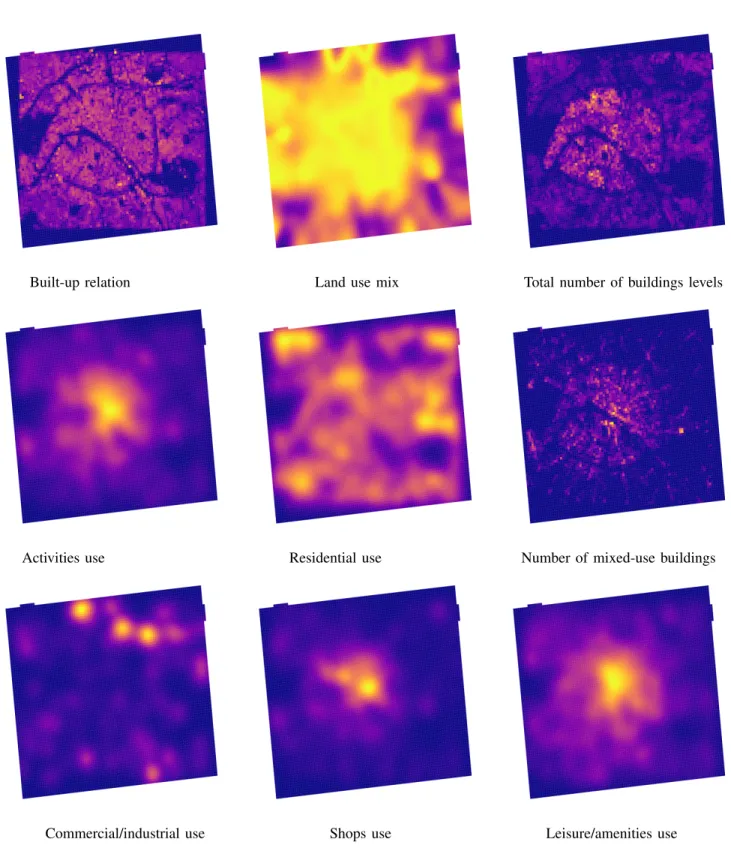
Built-up relation Land use mix Total number of buildings levels
Activities use Residential use Number of mixed-use buildings
Commercial/industrial use Shops use Leisure/amenities use
Fig. 6: Visual illustration of several computed urban features for the city of Paris, which will guide the population downscaling procedure.
resolution. A stand-alone whole city is kept out for the validation procedure, demonstrating that the proposed methods outperforms related work.
The code of the framework is open and available at7. Future
work includes enlarging the training and validation procedure throughout producing more ground-truth samples. This can be done by means of processing the whole French country – where the high resolution ground-truth exists which can be used for validation – or by means of processing other cities where fine-grained census tract data exists. In addition, other relevant urban features will be explored in order to enhance the model.
ACKNOWLEDGMENT
We gratefully acknowledge the support from the CNRS/IN2P3 Computing Center (Lyon/Villeurbanne -France) for providing the computing resources needed to carry out this work.
REFERENCES
[1] Z. Lu, J. Im, L. Quackenbush, and K. Halligan, “Population estimation based on multi-sensor data fusion,” International Journal of Remote Sensing, vol. 31, no. 21, pp. 5587–5604, 2010.
[2] S. Ural, E. Hussain, and J. Shan, “Building population mapping with aerial imagery and gis data,” International Journal of Applied Earth Observation and Geoinformation, vol. 13, no. 6, pp. 841–852, 2011. [3] M. Langford, “An evaluation of small area population estimation
tech-niques using open access ancillary data,” Geographical Analysis, vol. 45, no. 3, pp. 324–344, 2013.
[4] H. Sridharan and F. Qiu, “A spatially disaggregated areal interpolation model using light detection and ranging-derived building volumes,” Geographical Analysis, vol. 45, no. 3, pp. 238–258, 2013.
[5] W. Jifeng, L. Huapu, and P. Hu, “System dynamics model of urban transportation system and its application,” Journal of Transportation Systems engineering and information technology, vol. 8, no. 3, pp. 83– 89, 2008.
[6] P. Waddell, “Urbansim: Modeling urban development for land use, transportation, and environmental planning,” Journal of the American planning association, vol. 68, no. 3, pp. 297–314, 2002.
[7] M. Bakillah, S. Liang, A. Mobasheri, J. Jokar Arsanjani, and A. Zipf, “Fine-resolution population mapping using openstreetmap points-of-interest,” International Journal of Geographical Information Science, vol. 28, no. 9, pp. 1940–1963, 2014.
[8] J. Mennis, “Generating surface models of population using dasymetric mapping,” The Professional Geographer, vol. 55, no. 1, pp. 31–42, 2003. [9] M. Reibel and A. Agrawal, “Areal interpolation of population counts using pre-classified land cover data,” Population Research and Policy Review, vol. 26, no. 5-6, pp. 619–633, 2007.
[10] A. E. Gaughan, F. R. Stevens, C. Linard, P. Jia, and A. J. Tatem, “High resolution population distribution maps for southeast asia in 2010 and 2015,” PloS one, vol. 8, no. 2, p. e55882, 2013.
[11] F. Rodrigues, A. Alves, E. Polisciuc, S. Jiang, J. Ferreira, and F. Pereira, “Estimating disaggregated employment size from points-of-interest and census data: From mining the web to model implementation and visualization,” International Journal on Advances in Intelligent Systems, vol. 6, no. 1, pp. 41–52, 2013.
[12] P. Danoedoro, “Extracting land-use information related to socio-economic function from quickbird imagery: A case study of semarang area, indonesia,” Map Asia, vol. 2006, 2006.
[13] X. Liu, P. C. Kyriakidis, and M. F. Goodchild, “Population-density estimation using regression and area-to-point residual kriging,” Inter-national Journal of geographical information science, vol. 22, no. 4, pp. 431–447, 2008.
[14] S.-s. Wu, X. Qiu, and L. Wang, “Population estimation methods in gis and remote sensing: a review,” GIScience & Remote Sensing, vol. 42, no. 1, pp. 80–96, 2005.
7https://github.com/lgervasoni/urbansprawl
[15] F. R. Stevens, A. E. Gaughan, C. Linard, and A. J. Tatem, “Disag-gregating census data for population mapping using random forests with remotely-sensed and ancillary data,” PloS one, vol. 10, no. 2, p. e0107042, 2015.
[16] L. Gervasoni, S. Fenet, and P. Sturm, “Une m´ethode pour lestimation d´esagr´eg´ee de donn´ees de population `a laide de donn´ees ouvertes,” in 18`eme Conf´erence Internationale sur l’Extraction et la Gestion des Connaissances, 2018.
[17] C. Barrington-Leigh and A. Millard-Ball, “The worlds user-generated road map is more than 80% complete,” PloS ONE, vol. 12, no. 8, p. e0180698, 2017.
[18] H. Fan, A. Zipf, Q. Fu, and P. Neis, “Quality assessment for building footprints data on OpenStreetMap,” International Journal of Geograph-ical Information Science, vol. 28, no. 4, pp. 700–719, 2014.
[19] G. Touya, V. Antoniou, A.-M. Olteanu-Raimond, and M.-D. Van Damme, “Assessing crowdsourced poi quality: Combining methods based on reference data, history, and spatial relations,” ISPRS Interna-tional Journal of Geo-Information, vol. 6, no. 3, p. 80, 2017. [20] M. Haklay, “How good is volunteered geographical information? A
comparative study of OpenStreetMap and Ordnance Survey datasets,” Environment and Planning B: Planning and Design, vol. 37, no. 4, pp. 682–703, 2010.
[21] P. Neis, D. Zielstra, and A. Zipf, “The street network evolution of crowdsourced maps: OpenStreetMap in Germany 2007–2011,” Future Internet, vol. 4, no. 1, pp. 1–21, 2011.
[22] M. Over, A. Schilling, S. Neubauer, and A. Zipf, “Generating web-based 3D city models from OpenStreetMap: The current situation in Germany,” Computers, Environment and Urban Systems, vol. 34, no. 6, pp. 496–507, 2010.
[23] X. Liu and Y. Long, “Automated identification and characterization of parcels with OpenStreetMap and points of interest,” Environment and Planning B: Planning and Design, vol. 43, no. 2, pp. 341–360, 2016. [24] G. Boeing, “OSMnx: New methods for acquiring, constructing,
analyz-ing, and visualizing complex street networks,” Computers, Environment and Urban Systems, vol. 65, no. Supplement C, pp. 126 – 139, 2017. [25] L. Gervasoni, M. Bosch, S. Fenet, and P. Sturm, “A framework for
evaluating urban land use mix from crowd-sourcing data,” in Big Data (Big Data), 2016 IEEE International Conference on. IEEE, 2016, pp. 2147–2156.
[26] ——, “Calculating spatial urban sprawl indices using open data,” in 15th International Conference on Computers in Urban Planning and Urban Management, 2017.
[27] D. Ciregan, U. Meier, and J. Schmidhuber, “Multi-column deep neural networks for image classification,” in Computer vision and pattern recognition (CVPR), 2012 IEEE conference on. IEEE, 2012, pp. 3642– 3649.
[28] A. Krizhevsky, I. Sutskever, and G. E. Hinton, “Imagenet classification with deep convolutional neural networks,” in Advances in neural infor-mation processing systems, 2012, pp. 1097–1105.
[29] K. Makantasis, K. Karantzalos, A. Doulamis, and N. Doulamis, “Deep supervised learning for hyperspectral data classification through convolu-tional neural networks,” in Geoscience and Remote Sensing Symposium (IGARSS), 2015 IEEE International. IEEE, 2015, pp. 4959–4962.