HAL Id: hal-03048305
https://hal.archives-ouvertes.fr/hal-03048305
Submitted on 10 Dec 2020
HAL is a multi-disciplinary open access
archive for the deposit and dissemination of
sci-entific research documents, whether they are
pub-lished or not. The documents may come from
teaching and research institutions in France or
abroad, or from public or private research centers.
L’archive ouverte pluridisciplinaire HAL, est
destinée au dépôt et à la diffusion de documents
scientifiques de niveau recherche, publiés ou non,
émanant des établissements d’enseignement et de
recherche français ou étrangers, des laboratoires
publics ou privés.
Intercomparison Project (ACCMIP): overview and
description of models, simulations and climate
diagnostics
J.-F. Lamarque, D. Shindell, B. Josse, P. Young, I. Cionni, V. Eyring, D.
Bergmann, P. Cameron-Smith, W. Collins, R. Doherty, et al.
To cite this version:
J.-F. Lamarque, D. Shindell, B. Josse, P. Young, I. Cionni, et al.. The Atmospheric Chemistry and
Climate Model Intercomparison Project (ACCMIP): overview and description of models, simulations
and climate diagnostics. Geoscientific Model Development, European Geosciences Union, 2013, 6 (1),
pp.179-206. �10.5194/GMD-6-179-2013�. �hal-03048305�
Geosci. Model Dev., 6, 179–206, 2013 www.geosci-model-dev.net/6/179/2013/ doi:10.5194/gmd-6-179-2013
© Author(s) 2013. CC Attribution 3.0 License.
Advances in
Geosciences
Natural Hazards
and Earth System
Sciences
Open Access
Annales
Geophysicae
Nonlinear Processes
in Geophysics
Atmospheric
Chemistry
and Physics
Open AccessAtmospheric
Chemistry
and Physics
Open Access DiscussionsAtmospheric
Measurement
Techniques
Open AccessAtmospheric
Measurement
Techniques
Open Access DiscussionsBiogeosciences
Open Access Open Access
Biogeosciences
DiscussionsClimate
of the Past
Open Access Open Access
Climate
of the Past
Discussions
Earth System
Dynamics
Open Access Open Access
Earth System
Dynamics
DiscussionsGeoscientific
Instrumentation
Methods and
Data Systems
Open Access
Geoscientific
Instrumentation
Methods and
Data Systems
Open Access DiscussionsGeoscientific
Model Development
Open Access Open Access
Geoscientific
Model Development
DiscussionsHydrology and
Earth System
Sciences
Open AccessHydrology and
Earth System
Sciences
Open Access DiscussionsOcean Science
Open Access Open Access
Ocean Science
DiscussionsSolid Earth
Open Access Open Access
Solid Earth
Discussions
The Cryosphere
Open Access Open Access
The Cryosphere
Discussions
Natural Hazards
and Earth System
Sciences
Open Access
Discussions
The Atmospheric Chemistry and Climate Model Intercomparison
Project (ACCMIP): overview and description of models, simulations
and climate diagnostics
J.-F. Lamarque1, D. T. Shindell2, B. Josse3, P. J. Young4,5,*, I. Cionni6, V. Eyring7, D. Bergmann8, P. Cameron-Smith8, W. J. Collins9,**, R. Doherty10, S. Dalsoren11, G. Faluvegi2, G. Folberth9, S. J. Ghan12, L. W. Horowitz13, Y. H. Lee2, I. A. MacKenzie10, T. Nagashima14, V. Naik15, D. Plummer16, M. Righi7, S. T. Rumbold9, M. Schulz17, R. B. Skeie11, D. S. Stevenson10, S. Strode18,19, K. Sudo14, S. Szopa20, A. Voulgarakis21, and G. Zeng22
1NCAR Earth System Laboratory, National Center for Atmospheric Research, Boulder, CO, USA 2NASA Goddard Institute for Space Studies and Columbia Earth Institute, New York, NY, USA
3GAME/CNRM, M´et´eo-France, CNRS – Centre National de Recherches M´et´eorologiques, Toulouse, France
4Cooperative Institute for Research in the Environmental Sciences, University of Colorado-Boulder, Boulder, CO, USA 5Chemical Sciences Division, NOAA Earth System Research Laboratory, Boulder, CO, USA
6Agenzia nazionale per le nuove tecnologie, l’energia e lo sviluppo economico sostenibile (ENEA), Bologna, Italy 7Deutsches Zentrum f¨ur Luft- und Raumfahrt (DLR), Institut f¨ur Physik der Atmosph¨are, Oberpfaffenhofen, Germany 8Lawrence Livermore National Laboratory, Livermore, CA, USA
9Hadley Centre for Climate Prediction, Met Office, Exeter, UK 10School of Geosciences, University of Edinburgh, Edinburgh, UK
11Center for International Climate and Environmental Research-Oslo (CICERO), Oslo, Norway 12Pacific Northwest National Laboratory, Richland, WA, USA
13NOAA Geophysical Fluid Dynamics Laboratory, Princeton, NJ, USA
14Frontier Research Center for Global Change, Japan Marine Science and Technology Center, Yokohama, Japan
15UCAR/NOAA Geophysical Fluid Dynamics Laboratory, Princeton, NJ, USA
16Canadian Centre for Climate Modeling and Analysis, Environment Canada, Victoria, British Columbia, Canada 17Meteorologisk Institutt, Oslo, Norway
18NASA Goddard Space Flight Center, Greenbelt, MD, USA
19Universities Space Research Association, Columbia, MD, USA
20Laboratoire des Sciences du Climat et de l’Environnement, CEA/CNRS/UVSQ/IPSL, Gif-sur-Yvette, France 21Department of Physics, Imperial College, London, UK
22National Institute of Water and Atmospheric Research, Lauder, New Zealand *now at: Lancaster Environment Centre, Lancaster University, Lancaster, UK **now at: Department of Meteorology, University of Reading, UK
Correspondence to: J.-F. Lamarque ([email protected])
Received: 30 July 2012 – Published in Geosci. Model Dev. Discuss.: 28 August 2012 Revised: 21 December 2012 – Accepted: 7 January 2013 – Published: 7 February 2013
Abstract. The Atmospheric Chemistry and Climate Model
Intercomparison Project (ACCMIP) consists of a series of time slice experiments targeting the long-term changes in atmospheric composition between 1850 and 2100, with the goal of documenting composition changes and the associated
radiative forcing. In this overview paper, we introduce the ACCMIP activity, the various simulations performed (with a requested set of 14) and the associated model output. The 16 ACCMIP models have a wide range of horizontal and vertical resolutions, vertical extent, chemistry schemes and
Table 1. List and principal characteristics of ACCMIP simulations. Additional simulations (1890, 1910, 1950, 1970, and 1990) were proposed
as Optional and are removed from this table for clarity. SSTs stands for sea surface temperatures and GHGs for greenhouse gases.
Historical Simulations
Configuration 1850 1930 1980 2000 Name Emissions and SSTs/GHGs for given year P P P P acchist Year 2000 emissions except 1850 SSTs and GHGs P Em2000Cl1850 2000 case except 1850 CH4concentration O Em2000CH4185 2000 case except 1850 NOxemissions O Em2000NOx185
2000 case except 1850 CO emissions O Em2000CO1850 2000 case except 1850 NMHCs emissions O Em2000NMVOC185 Future Simulations
Emissions/Configuration 2010 2030 2050 2100 Name RCP 2.6 (emissions, GHGs and SSTs) P O P accrcp26 RCP 4.5 (emissions, GHGs and SSTs) O O O O accrcp45 RCP 6.0 (emissions, GHGs and SSTs) P P O P accrcp60 RCP 8.5 (emissions, GHGs and SSTs) P O P accrcp85 Year 2000 emissions/RCP 8.5 SSTs and GHGs for 2030 P Em2000Cl2030 Year 2000 emissions/RCP 8.5 SSTs and GHGs for 2100 P Em2000Cl2100 P = Primary, O = Optional, blank = not requested.
interaction with radiation and clouds. While anthropogenic and biomass burning emissions were specified for all time slices in the ACCMIP protocol, it is found that the natural emissions are responsible for a significant range across mod-els, mostly in the case of ozone precursors. The analysis of selected present-day climate diagnostics (precipitation, tem-perature, specific humidity and zonal wind) reveals biases consistent with state-of-the-art climate models. The model-to-model comparison of changes in temperature, specific hu-midity and zonal wind between 1850 and 2000 and between 2000 and 2100 indicates mostly consistent results. However, models that are clear outliers are different enough from the other models to significantly affect their simulation of atmo-spheric chemistry.
1 Introduction
The Coupled Model Intercomparison Project (CMIP) is a protocol for (1) systematically defining model simulations to be performed with coupled atmosphere–ocean general cir-culation models (AOGCMs) and (2) studying the generated output. This framework provides the scientific community with the ability to more easily and meaningfully intercom-pare model results, a process which serves to facilitate model improvement. The simulations performed for the Climate Model Intercomparison Project phase 3 (CMIP3) in support of the Intergovernmental Panel on Climate Change (IPCC) Fourth Assessment Report (AR4) have provided a useful resource for exploring issues of climate sensitivity, histori-cal climate and climate projections (e.g. Meehl et al., 2007 and references therein). However, the forcings imposed in
simulations of the past or of the future varied from model to model due to varying assumptions about emissions (Shin-dell et al., 2008), differences in the representation of physical and biogeochemical processes affecting short-lived species that were included (such as aerosols and tropospheric ozone and its precursors), and differences in which processes and constituents were included at all (Pendergrass and Hartmann, 2012). For example, only 8 of 23 CMIP3 models included black carbon while fewer than half included future tropo-spheric ozone changes. Furthermore, the CMIP3 archive does not include diagnostics of spatially variable radiative forcing from aerosols, ozone, or greenhouse gases other than carbon dioxide. Hence it is not straightforward to understand how much of the variation between simulated climates re-sults from internal climate sensitivity and inter-model differ-ences or from differdiffer-ences in their forcings.
Similarly to CMIP3, there are gaps in the output from CMIP Phase 5 (CMIP5; note that the naming convention for CMIP was changed to align itself with the IPCC AR num-bering, leading to the jump from CMIP3 to CMIP5) when it comes to atmospheric chemistry, with relatively little in-formation on aerosols or greenhouse gases requested from models (Taylor et al., 2012). In particular, despite having relatively uniform anthropogenic emissions, natural emis-sions are likely highly diverse. Concentrations (forcings) will also differ between models due to different transforma-tion/removal processes. This is especially the case as models progress towards a more Earth System approach and repre-sent interactions with the biosphere (Arneth et al., 2010a), including climate-sensitive emissions of isoprene (Guenther et al., 2006; Arneth et al., 2010b), methane (O’Connor et al.,
Fig. 1. Time evolution of global anthropogenic + biomass burning emissions 1850–2100 following each RCP; blue (RCP2.6), light blue (RCP4.5), orange (RCP6.0) and red (RCP8.5). BC represents black carbon (in Tg(C) yr−1), OC organic carbon (in Tg(C) yr−1), NMVOC non-methane volatile organic compounds (in Tg(C) yr−1) and NOxnitrogen oxides (in Tg(NO2) yr−1). Other panels are in Tg(species) yr−1.
Histori-cal (1850–2000) values are from Lamarque et al. (2010). RCP values are from van Vuuren et al. (2011) and references therein.
37
Fig. 1. Time evolution of global anthropogenic + biomass burning emissions 1850–2100 following each RCP; blue (RCP2.6), light blue
(RCP4.5), orange (RCP6.0) and red (RCP8.5). BC represents black carbon (in Tg(C) yr−1), OC organic carbon (in Tg(C) yr−1), NMVOC non-methane volatile organic compounds (in Tg(C) yr−1) and NOxnitrogen oxides (in Tg(NO2)yr−1). Other panels are in Tg(species) yr−1.
Historical (1850–2000) values are from Lamarque et al. (2010). RCP values are from van Vuuren et al. (2011) and references therein.
2010) and soil nitrogen (Steinkamp and Lawrence, 2011), as well as the more standard climate-sensitive lightning emis-sions. Hence there is a need for characterization of the forc-ings imposed in the CMIP5 historical and future simulations, and for diagnostics to help understanding the causes of the differences in forcings from model to model.
The Atmospheric Chemistry and Climate Model Inter-comparison Project (ACCMIP) aims to better evaluate the role of atmospheric chemistry in driving climate change, both gases and aerosols. Effectively, ACCMIP targets the analyses of the driving forces of climate change in the simu-lations being performed in CMIP5 (Taylor et al., 2012; note that in this document, ACCMIP is identified by the previ-ous acronym, AC&C#4) in support of the upcoming IPCC Fifth Assessment Report (AR5). After an initial meeting in 2009, ACCMIP was organized at an April 2011 workshop where simulations, requested output and associated proto-cols and analysis teams were thoroughly defined. ACCMIP consists of a set of numerical experiments designed to pro-vide insight into atmospheric chemistry driven changes in the
CMIP5 simulations of historical and future climate change, along with additional sensitivity simulations aiming to better understand the role of particular processes driving the non-CO2anthropogenic climate forcing (such as the aerosol in-direct effects and the effects of specific precursors on tropo-spheric ozone). Finally, through its multi-model setup, AC-CMIP provides a range in forcing estimates.
In addition, ACCMIP benefits from a wealth of new and updated observations related to atmospheric chemistry to evaluate and further our understanding of processes link-ing chemistry and climate. ACCMIP studies take advan-tage of these measurements by performing model evalua-tions, especially with respect to their simulations of tropo-spheric ozone and aerosols, both of which have substantial climate forcing that varies widely in space and time (Shindell et al., 2012). For this purpose, observations such as retrievals from the Tropospheric Emission Spectrometer (TES), the Ozone Monitoring Instrument (OMI), the Moderate Res-olution Imaging Spectroradiometer (MODIS) on the Aura satellite, the Cloud-Aerosol Lidar and Infrared Pathfinder
Table 2. List of participating models to and ACCMIP simulations performed. The number of years (valid for each experiment) is listed in
the acchist 2000 column.
acchist accrcp26 accrcp45 accrcp60 accrcp85 Model 1850 1930 1980 2000 2030 2100 2030 2100 2010 2030 2100 2030 2100 CESM-CAM-Superfast X X X 10 X X X X X X X CICERO X X X 1 X X X X X X CMAM X X 10 X X X X EMAC-DLR X X X 10 X X X X GEOSCCM X X 14 X GFDL-AM3 X X 10 X X X X X X X X GISS-E2-R X X X 11 X X X X X X X X X GISS-E2-R-TOMAS X X X 10 HADGEM2 X X 10 X X X LMDZORINCA X X X 11 X X X X X X X X X MIROC-CHEM X X X 10 X X X X X X X MOCAGE X X X 4 X X X X X X X NCAR-CAM3.5 X X X 8 X X X X X X X X NCAR-CAM5.1 X X X 10 STOC-HadAM3 X X X 10 X X X X UM-CAM X X X 10 X X X X X X
Model Em2000 Em2000 Em2000 Em2000 Em2000 Em2000 Em2000 Cl1850 CH41850 NOx1850 CO1850 NMVOC1850 Cl2030 Cl2100
CESM-CAM-Superfast X X X CICERO X X X X CMAM EMAC-DLR X X X GEOSCCM GFDL-AM3 X X X X GISS-E2-R GISS-E2-R-TOMAS HADGEM2 LMDZORINCA MIROC-CHEM MOCAGE X X X NCAR-CAM3.5 X X X X X X X NCAR-CAM5.1 X STOC-HadAM3 UM-CAM X X X X X X X
Satellite Observations (CALIPSO), and the ground-based Aerosol Robotic Network (Aeronet) will be used.
This paper is the ACCMIP overview paper and as such serves as a central repository of information relevant to the ACCMIP simulations (of which 14 were requested), the 16 models performing them and the various ACCMIP pa-pers presently submitted to the Atmospheric Chemistry and Physics ACCMIP Special Issue, discussing (1) aerosols and total radiative forcing (Shindell et al., 2012a), (2) histori-cal and future changes in tropospheric ozone (Young et al., 2012), (3) tropospheric ozone radiative forcing and attribu-tion (Stevenson et al., 2012), (4) ozone comparison with TES (Bowman et al., 2012), (5) black carbon deposition (Lee et al., 2012) and (6) OH (hydroxyl radical) and methane life-time in the historical (Naik et al., 2012a) and future (Voul-garakis et al., 2012) simulations. As such, we present here only the overall suite of model characteristics, simulations performed and evaluation of selected climate variables, since the evaluation and analysis of chemical composition and in-depth model descriptions will be addressed as needed in each paper.
The paper is organized as follows: in Sect. 2, we provide an overview of the ACCMIP simulations. Section 3 describes the main characteristics of the participating models. Sec-tion 4 focuses on the evaluaSec-tion of the present-day simula-tions against observasimula-tions, with a particular focus on selected physical climate variables (precipitation, specific humidity, temperature and zonal wind). Section 5 provides a descrip-tion of the climate response to simulated historical and pro-jected changes in the same physical climate variables. Sec-tion 6 presents a brief discussion and overall conclusions.
2 Description of simulations, output protocol and data access
The ACCMIP simulations (Table 1) consist of time slice ex-periments (for specific periods spanning 1850 to 2100 with a minimum increment of 10 yr) with chemistry diagnostics, providing information on the anthropogenic forcing of his-torical and future climate change in the CMIP5 simulations, including the chemical composition changes associated with this forcing. Each requested simulation is labeled as Primary
Fig. 2. Time evolution of global-averaged mixing ratio of long-lived species1850–2100 following each RCP; blue (RCP2.6), light blue (RCP4.5), orange (RCP6.0) and red (RCP8.5). ClOy and BrOy are the total organic chlorine and bromine compounds, respectively, summarizing the evolution of ozone-depleting substances. All values from Meinshausen et al. (2011).
38
Fig. 2. Time evolution of global-averaged mixing ratio of long-lived species 1850–2100 following each RCP; blue (RCP2.6), light blue
(RCP4.5), orange (RCP6.0) and red (RCP8.5). ClOy and BrOy are the total organic chlorine and bromine compounds, respectively, summa-rizing the evolution of ozone-depleting substances. All values from Meinshausen et al. (2011).
(“P”) or Optional (“O”). Note that additional simulations (ad-ditional time slices or sensitivity tests) were performed by only a limited number of modeling groups. For clarity, they are not listed in Table 1 but will be referred to in some of the ACCMIP papers.
Figures 1 and 2 show the prescribed evolution of short-lived precursor emissions and long-short-lived specie concentra-tions for the different periods and scenarios in the study. For the historical period, beyond the “pre-industrial” tative of year 1850 emissions) and “present-day” (represen-tative of year 2000 emissions) time slices, we have included 1930 (beginning of the large increase in global anthropogenic emissions) and 1980 (peak in anthropogenic emissions over Europe and North America).
Projection simulations follow the Representative Concen-tration Pathways (RCPs; van Vuuren et al., 2011 and ref-erences therein) for both short-lived precursor emissions (Fig. 1) and long-lived specie concentrations (Fig. 2; Mein-shausen et al., 2011). Amongst the 4 available RCPs, a higher simulation priority was given to RCP6.0 since it has short-lived precursor emissions significantly different from the other RCPs, especially in the first half of the 21st century (Fig. 1); however, RCP2.6 and RCP8.5 are still scientifically important since they provide the extremes in terms of 2100 climate change and methane levels. In addition to the pri-mary simulations at 2030 and 2100, an optional time slice at 2050 is included as this time horizon is of interest to policy makers.
Additional simulations were completed, using 2000 emis-sions but with an 1850, 2030 and 2100 (both with RCP8.5) climate, to separate the effects of climate change and
CO 1850 1980 2000 time slice 400 600 800 NMHCs 1850 1980 2000 time slice 200 400 600 800 1000 1200 1400 1600 Tg yr-1 1000 Tg C yr -1 1200 1800 Total NOx 1850 1980 2000 time slice 10 20 30 40 50 60 Lightning NOx 1850 1980 2000 time slice 2 4 6 8 10 Tg N yr-1 Tg N yr-1
Fig. 3. Time evolution of historical total (anthropogenic + biomass burning + natural) emissions of NOx, CO and NMHCs. In addition, lightning emissions are shown. For each time slice, the filled circle indicates the mean, the solid line the median, the extent of the box is 25–75 % and minimum and maximum are shown (adapted from Young et al., 2012).
39
Fig. 3. Time evolution of historical total (anthropogenic + biomass
burning + natural) emissions of NOx, CO and NMHCs. In addition,
lightning emissions are shown. For each time slice, the filled circle indicates the mean, the solid line the median, the extent of the box is 25–75 % and minimum and maximum are shown (adapted from Young et al., 2012).
emissions on constituents and for isolating aerosol indirect effects. In these, the sea surface temperatures and long-lived specie concentrations were specified following their values in the target climate.
Table 3. Model description summary.
Model Modelling Center Model Contact Reference 1 CESM-CAM-Superfast LLNL, USA Dan Bergmann Lamarque et al. (2012)
Philip Cameron-Smith
2 CICERO-OsloCTM2 CICERO, Norway Stig Dalsoren Skeie et al. (2011a, b) Ragnhild Skeie
3 CMAM CCCMA, Environment David Plummer Scinocca et al. (2008) Canada, Canada
4 EMAC DLR, Germany Patrick J¨ockel, J¨ockel et al. (2006) Veronika Eyring
Mattia Righi Irene Cionni
5 GEOSCCM NASA GSFC, USA Sarah Strode Oman et al. (2011) 6 GFDL-AM3 UCAR/NOAA, Larry Horowitz, Donner et al. (2011)
GFDL, USA Vaishali Naik Naik et al. (2012b) 7 GISS-E2-R(-TOMAS) NASA-GISS,USA Drew Shindell Koch et al. (2006)
Greg Faluvegi Shindell et al. (2012b) 8 GISS-E2-R-TOMAS NASA-GISS,USA Drew Shindell Lee and Adams (2011) Greg Faluvegi Shindell et al. (2012b)
Yunha Lee
9 HadGEM2 Hadley Center, William Collins Collins et al. (2011) Met.Office, UK Gerd Folbert
Steve Rumbold
10 LMDzORINCA LSCE, CEA/CNRS Sophie Szopa Szopa et al. (2012) /UVSQ/IPSL, France
11 MIROC-CHEM FRCGC, JMSTC Tatsuya Nagashima Watanabe et al. (2011) Japan Kengo Sudo
12 MOCAGE GAME/CNRM B´eatrice Josse Josse et al. (2004) M´et´eoFrance, France Teyss`edre et al. (2007) 13 NCAR-CAM3.5 NCAR,USA Jean-Franc¸ois Lamarque Lamarque et al. (2011, 2012) 14 NCAR-CAM5.1 PNNL, USA Steve Ghan X. Liu et al. (2012) 15 STOC-HadAM3 University of Ian McKenzie Stevenson et al. (2004)
Edinburgh,UK David Stevenson Ruth Doherty
16 UM-CAM NIWA, New Zealand Guang Zeng Zeng et al. (2008, 2010)
As variations in the solar activity since 1850 is of lim-ited importance for tropospheric chemistry, no specifica-tion was made in the ACCMIP protocol. Suggested vol-canoes and associated stratospheric surface area density follow CCMVal (http://www.pa.op.dlr.de/CCMVal/Forcings/ CCMVal Forcings WMO2010.html), with no volcanic erup-tions in the future.
The proposed simulation length was 4–10 yr (excluding spinup, see Table 2) using prescribed monthly sea surface temperature (SST) and sea ice concentration (SIC) distri-butions, valid for each time slice and averaged over 10 yr. This averaging was designed to reduce the effect of inter-annual variability and therefore provide optimal conditions from which average composition changes and associated forcings can be more readily computed. Output from tran-sient simulations performed with two coupled chemistry– climate–ocean models (i.e. CMIP5 runs, performed by GISS-E2-R and LMDzORINCA) is also part of the ACCMIP data
collection. For the analysis of these models, output fields were averaged over an 11-yr window centered on the target time-slice year (e.g. 2025–2035 for the 2030 time slice).
2.1 Emissions and concentration boundary conditions
Consistent gridded emissions data from 1850 to 2100 were created in support of CMIP5 and of this activity; the his-torical (1850–2000) portion of this dataset is discussed in Lamarque et al. (2010). The year 2000 dataset was used for harmonization with the future emissions determined by In-tegrated Assessment Models (IAMs) for the four RCPs de-scribed in van Vuuren et al. (2011) and references therein. As shown in Fig. 1, all emissions necessary for the simula-tion of tropospheric ozone and aerosols between 1850 and 2100 are available for both anthropogenic activities (includ-ing biofuel, shipp(includ-ing and aircraft) and biomass burn(includ-ing.
Model Type Resolution (lat/lon/# levels), Methane Top level
CESM-CAM-Superfast CCM 1.875/2.5/L26, 3.5 hPa Prescribed atmospheric concentrations with spatial variation, different for each time slice
CICERO-OsloCTM2 CTM 2.8/2.8/L60, 0.11 hPa Prescribed surface concentrations - zonal averages from IPCC TAR for historical; CMIP5 surface concentrations scaled to be consistent with present-day levels in the historical simulations for RCP simulations
CMAM CCM 3.75/3.75/L71, 0.00081 hPa Prescribed year-specific surface concentrations follow-ing CMIP5. Different in each time slice
EMAC CCM T42/L90, 0.01 hPa Prescribed surface concentrations (following CMIP5), different in each time slice
GEOSCCM CCM 2/2.5/L72, 0.01 hPa Prescribed surface (two bottom levels) concentrations. Surface methane has a prescribed latitudinal gradient, normalized to match the CMIP5 value at the time slice period
GFDL-AM3 CCM 2/2.5/L48, 0.017 hPa Prescribed surface concentrations (following CMIP5), different in each time slice
GISS-E2-R(-TOMAS) CCM 2/2.5/L40, 0.14 hPa Prescribed surface concentrations for historical (follow-ing CMIP5), emissions for future
HadGEM2 CCM 1.24/1.87/L38, hPa Prescribed surface concentrations LMDzORINCA CCM 1.9/3.75/L19, hPa Emissions for historical and future
MIROC-CHEM CCM 2.8/2.8/L80, 0.003 hPa Prescribed surface concentrations (following CMIP5), different in each time slice
MOCAGE CTM 2.0/2.0/L47, 6.9 hPa Prescribed surface concentrations (following CMIP5), different in each time slice
NCAR-CAM3.5 CCM 1.875/2.5/L26, 3.5 hPa Prescribed surface concentrations (following CMIP5), different in each time slice
NCAR-CAM5.1 CCM 1.875/2.5/L30, 3.5 hPa Prescribed distributions from NCAR-CAM3.5 STOC-HadAM3 CGCM 5.0/5.0/L19, 50 hPa Prescribed globally uniform CH4concentrations.
Different for each time slice following CMIP5 dataset UM-CAM CGCM 2.5/3.75/L19, 4.6 hPa Prescribed atmospheric concentration with no spatial
variation; different for each time slice
Concentrations of long-lived chemical species and green-house gases were based on the observed historical record (1850–2005) and on the RCP emissions, converted to con-centrations by Meinshausen et al. (2011) and shown in Fig. 2. Unlike anthropogenic and biomass burning emissions, nat-ural emissions (mostly isoprene, lightning and soil NOx, oceanic emissions of CO, dimethylsulfide, NH3, and emis-sions of non-erupting volcanoes) were not specified. No at-tempts were made at harmonizing natural emissions between modeling groups, leading to a range in emissions (Fig. 3). A summary of the emissions as implemented in each model is listed in Table 3 and further discussion on variations be-tween model natural emissions is provided in Sect. 3.
2.2 Simulation output
The ACCMIP simulations provide as output the concen-tration or mass of radiatively active species, aerosol opti-cal properties, and radiative forcings (clear and all sky).
Furthermore, the output also includes important diagnostics to document these, such as the hydroxyl radical concen-tration, photolysis rates, various ozone budget terms (e.g. production and loss rates and dry deposition flux), spe-cific chemical reaction rates, nitrogen and sulfate deposition rates, emission rates, high-frequency (hourly) surface pollu-tant concentrations (O3, NO2and PM2.5) and diagnostics of tracer transport. A complete list of the monthly output is pro-vided as Table S1. For all variables, Climate Model Output Rewriter (CMOR, see http://www2-pcmdi.llnl.gov/cmor) ta-bles have been created, based in part on protocols defined for previous model intercomparisons, such as Hemispheric Transport of Air Pollutants (HTAP, see http://www.htap. org), Aerosol Comparisons between Observations and Mod-els (AeroCOM, see http://aerocom.met.no/), and Chemistry-Climate Model Validation (CCMVal, see http://www.pa.op. dlr.de/CCMVal). All ACCMIP-generated data follow stan-dardized netCDF formats and use Climate and Forecast (CF;
Table 3. Continued.
Model Lightning NOx Other Natural emissions
CESM-CAM-Superfast Interactive, based on model’s convection (Price et al., 1997)
Constant present-day isoprene, CH2O, soil
NOx, DMS and volcanic sulfur, oceanic CO
CICERO-OsloCTM2 Interactive, based on model’s convection (Price et al., 1997) and scaled to 5 Tg N yr−1
Constant present-day (year 2000). From the RETRO dataset: CO, NOx, C2H4,C2H6,
C3H6, C3H8, ISOPRENE, ACETONE.
Vari-ous datasets: SO2, H2S, DMS,TERPENES, sea salt, NH3
CMAM Interactive, based on convective updraft mass flux (modified version of Allen and Pickering, 2002)
Constant; pre-industrial soil NOxemission of
8.7 Tg N yr−1 plus CMIP5 Agriculture (soil) anthropogenic enhancement; CO emissions of 250 Tg CO yr−1as proxy for isoprene oxidation distributed as Guenther et al. (1995)
EMAC Interactive, updraft velocity as a measure of convective strength and associated cloud elec-trification with the flash frequency (Grewe et al., 2001)
Climate sensitive soil NOx, isoprene and
light-ning NOx and soil NO. Constant present-day
(year 2000) SO2 emissions from volcanoes
(Dentener et al., 2006), biogenic emissions of CO and VOC (Ganzeveld et al., 2006), terres-trial DMS (Spiro et al., 1992)
GEOSCCM Fixed emissions with a monthly climatology based on Price et al., scaled to 5 Tg N yr−1
Climate-sensitive soil NOxand biogenic VOC
emissions of isoprene and CO from monoter-pene. Biogenic propene and CO from methanol is scaled from isoprene. No oceanic CO GFDL-AM3 Interactive, based on model’s convection (Price
et al., 1997), scaled to produce ∼ 3–5 Tg N.
constant pre-industrial soil NOx; constant
present-day soil and oceanic CO, and biogenic VOC; climate-sensitive dust, sea salt, and DMS GISS-E2-R
(-TOMAS)
Interactive, based on model’s convection (mod-ified from Price et al., 1997)
Climate-sensitive isoprene based on present-day vegetation, climate sensitive dust, sea salt, DMS; constant present-day soil NOx, alkenes,
paraffin HadGEM2 Interactive, based on model’s convection (Price
and Rind, 1992)
Prescribed: soil NOx, BVOC (as CO), DMS
Climate sensitive: sea salt, dust LMDzORINCA Interactive, based on model’s convection (Price
et al., 1997)
Constant soil NOx, oceanic CO (no soil
CO) and oxygenated biogenic compounds for present-day
MIROC-CHEM Interactive, based on model’s convection based on Price and Rind (1992)
Constant present-day VOCs, soil-Nox, oceanic-CO (no soil oceanic-CO); climate-sensitive dust, sea salt, DMS
MOCAGE Climate sensitive (based on Price and Rind, 1992 and Ridley et al., 2005)
Constant present-day isoprene, Other VOCs, Oceanic CO, Soil NOx
NCAR-CAM3.5 Interactive, based on model’s convection (Price et al., 1997; Ridley et al., 2005), scaled to pro-duce ∼ 3–5 Tg N.
Constant pre-industrial soil NOx emissions,
constant present-day biogenic isoprene, bio-genic and oceanic CO, other VOCs and DMS; climate-sensitive dust, sea salt
NCAR-CAM5.1 NA Sea salt, DMS, mineral dust, wildfire BC&POA, smoldering volcanic SO2
STOC-HadAM3 Interactive, based on model’s convection (Price and Rind, 1992; Price et al., 1997)
Constant, present-day emissions of NO, CO, NH3, VOC, DMS and H2 from veg, soil
and ocean. Present-day volcanic SO2.
Climate-sensitive isoprene UM-CAM Climate sensitive; based on parameterization
from Price and Rind (1997)
Constant present-day biogenic isoprene, soil NOx, biogenic and oceanic CO
Model SSTs/SICE
CESM-CAM-Superfast Decadal means from fully coupled CESM-CAM model simulation for CMIP5, except for the RCP2.6 and RCP6.0 simulations which used SSTs from an earlier version (CCSM3)
CICERO-OsloCTM2 CTM. Met fields: Forecast data for year 2006 from ECMWF IFS model CMAM Decadal means from two members of CCCma CanESM2 CMIP5 simulations EMAC Decadal means from the CMIP5 run carried out with the CMCC Climate Model
GEOSCCM 1870s AMIP SSTs for the 1850 time slice, http://www-pcmdi.llnl.gov/projects/amip/ AMIP2EXPDSN/BCS/bcsintro.php, based on HadISST v1 and NOAA OI SST v2 (Hurrell et al., 2008). SSTs from the CCSM4 for 2100 RCP60 time slice (Meehl et al., 2012)
GFDL-AM3 Decadal mean SSTs/SICE from one member of GFDL-CM3 CMIP5 simulations GISS-E2-R(-TOMAS) Transient, with simulated SSTs/SICE (CMIP5/ACCMIP runs)
HadGEM2 HadGEM2 CMIP5 transient run for the appropriate time period (Jones et al., 2011).
LMDzORINCA SSTs/SICE from HadiSST for historical and from AR4 simulations of IPSL-CM4 ESM (B1, A1B, and A2 for 4.5, 6.0, and 8.5, respectively, and scenario E1 (van Vuuren et al., 2007) for RCP2.6)
MIROC-CHEM monthly mean SSTs/SICE from MIROC-ESM CMIP5 simulations; data for the corresponding ACCMIP time slice year is used and repeated over the years of model integration
MOCAGE No SSTs/SICE (CTM); met. fields taken from atmosphere-only ARPEGE-Climate runs, using SSTs/SICE from CMIP5 runs
NCAR-CAM3.5 SSTs/SICE from AR4 CCSM3 simulations (historical and SRES 2000 commitment, B1, A1B, and A2 for RCP 2.6, 4.5, 6.0, and 8.5, respectively)
NCAR-CAM5.1 Decadal mean SST/Sea ice from fully coupled CESM-CAM5 model simulation for CMIP5 STOC-HadAM3 Same as HadGEM2
UM-CAM Same as HadGEM2
http://cf-pcmdi.llnl.gov) compliant names whenever avail-able.
Not every model performed all simulations, even the pri-mary ones. The overall availability of results for each model and each simulation is shown in Table 2. Data are cur-rently archived at the British Atmospheric Data Centre (see http://badc.nerc.ac.uk), with a data access policy provid-ing one year of access to participatprovid-ing groups only, fol-lowed by general public access to be granted no later than 31 July 2013.
3 Model description
In this section, we provide an overview of the 16 models that participated in ACCMIP simulations. In addition to these, the CSIRO-Mk3.6 CCM (Rotstayn et al., 2012) provided a lim-ited set of diagnostics and is included in the aerosol analysis of Shindell et al. (2012a). Also, results from the TM5 model (Huijnen et al., 2010) are used in Stevenson et al. (2012). The overview discusses the main aspects of relevance to chem-istry and atmospheric chemical composition. A more exten-sive description of each model is available as Supplement.
3.1 General discussion
The participating models are listed in Table 3. Of those, two are identified as Chemistry Transport Models (CTMs,
i.e. driven by externally specified meteorological fields from analysis – CICERO-OsloCTM2, or climate model fields – MOCAGE). Two others (UM-CAM and STOC-HadAM3) are referred to as Chemistry-General Circulation Models (CGCMs): they provide both prognostic meteorological and chemical fields, but chemistry does not affect climate. All other models are identified as Chemistry Climate Models (CCMs): in this case, simulated chemical fields (in addition to water vapour) are used in the radiation calculations and hence give a forcing on the general circulation of the atmo-sphere. Aerosol indirect effects are available in all classes of models.
In several cases, different models share many aspects: UM-CAM and Had-GEM2 use different dynamical cores, but share many parameterizations such as convection and the boundary layer scheme. On the other hand, UM-CAM and STOC-HadAM3 share the same dynamical core. A high degree of similarity is also found in E2-R and GISS-E2-R-TOMAS (different aerosol scheme; we will use the terminology GISS-E2s when common characteristics are discussed) and NCAR-CAM3.5 and CESM-CAM-Superfast (different chemistry scheme). Also, NCAR-CAM3.5 and NCAR-CAM5.1 share the same dynamical core and several physics parameterizations but differ in their representation of clouds, radiation and boundary-layer processes; these mod-els can be considered as distinct.
Table 3. Continued.
Model Composition-Radiation
Coupling
Photolysis scheme
CESM-CAM-Superfast Online H2O, O3, SO4; offline O2, CO2, N2O, CH4, CFC11, CFC12, BC, OC, dust, sea salt
Look-up table with correction for modeled clouds, stratospheric O3and surface albedo, not aerosols.
CICERO-OsloCTM2 No coupling (CTM) Online using the Fast-J2 (Wild et al., 2000; Bian and Prather, 2002); accounts for modeled O3, clouds, sur-face albedo and aerosols
CMAM Online O3, H2O; offline CO2, CH4, N2O, CFC-11 and CFC-12
Look-up table depending on modeled strat. O3and sur-face albedo; correction for clouds (follows Chang et al., 1987)
EMAC Online O3, H2O, SO4, CH4, CFCs; cli-matological aerosols
Online calculations of photolysis rate coefficients (J-values) using cloud water and ice content, cloudiness and climatological aerosol (J¨ockel et al., 2006) GEOSCCM online H2O, O3, N2O, CH4,
CFC-11,CFC-12,HCFC-22; offline aerosols
Online (FastJX); accounts for clouds, strat O3, and albedo; uses offline aerosols from GOCART
GFDL-AM3 Online H2O, O3, SO4, BC/OC, SOA, sea salt, dust; offline CH4, CFCs, N2O, CO2
Look-up table, based on TUV (v4.4); frequencies ad-justed for modeled clouds, strat. O3, and surface albedo, not for aerosols
GISS-E2-R(-TOMAS) Online H2O, O3, SO4, BC/OC, sea salt, dust, NO3; offline/online CH4 for his-torical/future; offline CO2, N2O, CFCs;
Online (Fast-J2 scheme); accounts for modeled clouds, strat. O3, aerosols, surface albedo
HadGEM2 Online tropospheric O3, CH4, H2O, SO4, BC, OC, dust; offline CFCs, N2O, strat O3
Look-up table (Law and Pyle, 1993); no correction for modeled fields
LMDzORINCA Offline CO2, CH4, CFC and N2O; no aerosol interactions
Look-up table, based on TUV (v4.1); frequencies ad-justed for modeled clouds, strat. O3, and surface albedo, not for aerosols
MIROC-CHEM Online H2O, O3, SO4, BC/OC, sea salt, dust, CFCs, N2O; offline CH4, CO2
Online coupled with radiation code considering gas absorption and cloud/aerosol/surface albedo, based on Landgraf and Crutzen (1998)
MOCAGE No coupling (CTM) Look-up table with correction for modeled clouds, stratospheric O3and surface albedo, not aerosols NCAR-CAM3.5 Online H2O, O3, SO4, BC/OC, SOA,
sea salt, dust, CH4, CFCs, N2O; offline CO2
Look-up table with correction for modeled clouds, stratospheric O3and surface albedo, not aerosols
NCAR-CAM5.1 Online H2O, aerosol with water uptake by κ-Kohler
NA
STOC-HadAM3 No coupling (CTM) 1-D, two-stream model (Hough, 1988). Uses climato-logical ozone above tropopause and modelled ozone be-low
UM-CAM Offline O3 (CMIP5 database), CH4, CO2, N2O, CFCs
Look-up table (Law and Pyle, 1993); no correction for modeled fields
Different grid structures are used for the horizontal dis-cretization. EMAC and CICERO-OsloCTM2 are based on a quadratic Gaussian grid of approximately 2.8◦, i.e. a spher-ical truncation of T42. CMAM is also a spectral model and was run at T47, though uses a regular grid (3.8 × 3.8 degree) for physical parameterizations. GFDL-AM3 has a horizontal domain consisting of a 6×48×48 cubed sphere-grid, with the grid size varying from 163 km (at the 6 corners of the cubed sphere) to 231 km (near the centre of each face). All remain-ing models use a regular latitude-longitude grid rangremain-ing from 1.25◦×1.875◦(HadGEM2) to 2.5◦×3.75◦(STOC-Hadam3
and UM-CAM). While the physics calculations in STOC-HadAM3 are performed at 2.5◦×3.75◦, this model uses a La-grangian chemical transport scheme, after which the fields are remapped onto a 5◦×5◦grid for output. While the hor-izontal resolutions are relatively homogeneous, the models have a greater range of vertical extent and resolution. Top levels range from 50 hPa (STOC-HadAM3) to 0.0081 hPa (CMAM), with a number of levels varying from 19 (LMD-zORINCA, STOC-HadAM3 and UM-CAM) to 90 (EMAC) (Fig. 4).
Model Species simulated Stratospheric Ozone CESM-CAM-Superfast 16 gas species; interactive sulfate; no aerosol indirect
effects
Linearized ozone chemistry
CICERO-OsloCTM2 93 gas species; BC, OC, sea salt, nitrate, sulfate, sec-ondary organic aerosols
Synoz. O3flux 450 Tg yr−1
CMAM 42 gas-phase species; No prognostic aerosols; specified monthly average sulphate distribution for hydrolysis re-actions
Full stratospheric chemistry
EMAC 96 gas-phase species, 8 additional species and 41 reac-tions for liquid phase chemistry, no prognostic aerosol
Full stratospheric chemistry
GEOSCCM No aerosols, 120 gas-phase species Full stratospheric chemistry GFDL-AM3 81 gas species; interactive SOx, BC/OC, SOA, NH3,
NO3, sea salt and dust; AIE included
Full stratospheric chemistry
GISS-E2-R (-TOMAS)
51 gas species; interactive sulfate, BC, OC, sea salt, dust, NO3, SOA; AIE included
Full stratospheric chemistry
HadGEM2 Interactive SO4, BC, OC, sea salt, dust; AIE included.
41 species
Offline stratospheric O3 from
CMIP5 dataset
LMDzORINCA 82 gas species; no aerosols Offline stratospheric O3
(climatol-ogy from Li and Shine, 1995) MIROC-CHEM 58 gas species; SO4, BC, OC, sea salt, dust; AIE
in-cluded
Full stratospheric chemistry
MOCAGE 110 gas species; no aerosols Full stratospheric chemistry NCAR-CAM3.5 117 gas species; BC, OC, SO4, NO3, SOA, dust, sea
salt
Full stratospheric chemistry
NCAR-CAM5.1 DMS, SO2, H2SO4gas SO4, BC, SOA, POA, sea salt,
and mineral dust aerosol internally mixed in 3 modes with predicted number. AIE included.
Prescribed distributions from NCAR-CAM3.5
STOC-HadAM3 65 gas phase species, SO4and NO3aerosol Offline stratospheric O3 from CMIP5 dataset
UM-CAM 60 gas phase species; no aerosols Offline stratospheric ozone from CMIP5 dataset
3.2 Deep convection
In CCMs, various convection schemes are used:
Tiedtke (1989) for EMAC, Gregory and Rowntree (1990) for Had-GEM2 and GISS-E2s, Arakawa-Schubert for GEOSCCM (Moorthi and Suarez, 1992), Emanuel (1991, 1993) for LMDzORINCA, and Zhang and McFarlane (1995) for CMAM, CESM-CAM-Superfast, NCAR-CAM3.5 and NCAR-CAM5.1.
In CGCMs, the convective diagnostics are obtained from the driving GCM, following Gregory and Rowntree (1990) in the case of UM-CAM and Collins et al. (2002; this model uses convective mass fluxes from HadAM3 to derive the probability of a parcel being subject to convective transport) in the case of STOC-HadAM3. CICERO-OsloCTM2 uses the convective mass flux (based on the Tiedtke, 1989 param-eterization) from the ECMWF Integrated Forecast System (IFS). MOCAGE re-computes its own distribution of con-vection using Bechtold et al. (2001).
All these parameterizations are based on the mass-flux ap-proach. However, Scinocca and McFarlane (2004) showed
that even with a single scheme, there is a wide variation in behaviour depending on details such as closure of the cloud-base mass flux. Furthermore, implementation details in the transport of tracers will make the impact of convection dif-ferent between models. The variations in representing deep convection as well as any shallow convection processes can therefore be a source of inter-model differences with respect to the vertical transport of chemical constituents, especially in the tropical regions. Unfortunately, very few models pro-vided convective mass flux as output and a more complete discussion cannot take place without additional simulations.
3.3 Wet and dry deposition
Wet removal and deposition of chemical species depends on their solubility, itself defined in terms of their Henry’s law effective coefficient, for gases and their hygroscopic-ity for aerosols. Removal by both large-scale and convec-tive precipitation is taken into account. Many models fol-low a first-order loss parameterization (e.g. Giannakopoulous et al., 1999). In Oslo-CTM2 only rainout, i.e. scavenging in
Table 3. Continued.
Model NMHCs
CESM-CAM-Superfast Isoprene only
CICERO-OsloCTM2 C2H4, C2H6, C3H6, C3H8, C4H10 (butanes + pentanes), C6H14, hexanes + higher alkanes), CH2O, CH3CHO (other alkanals), ACETONE (ketones), AROMATICS (benzene + toluene +
trimethylbenzenes + xylene +other aromatics), isoprene, terpenes
CMAM None
EMAC Up to isoprene
GEOSCCM MEK (> C3 ketones), PRPE (propene and ≥ C3 alkenes), C2H6, C3H8, CH2O, ALK4 (≥ C4 alkanes), acetaldehyde, isoprene, monoterpene, biogenic propene
GFDL-AM3 Monoterpenes, C2H4, C2H5OH, C2H6, C3H6(C > 3 alkenes), C3H8, C4H10(C > 4 alkanes), CH2O, CH3COCH3, CH3OH, and isoprene
GISS-E2-R (-TOMAS)
Isoprene, terpernes, alkenes (propene, other alkenes and alkynes, ethene), paraffin (propane, pentanes, butanes, hexanes and higher alkanes, ethane, ketones)
HadGEM2 Up to propane
LMDzORINCA Isoprene, Terpenes, CH3OH, C2H5OH, C2H6, C3H8, ALKAN, C2H4, C3H6, C2H2, ALKEN,,
AROM, CH2O, CH3CHO, CH3COCH3, MEK, MVK, CH3COOH
MIROC-CHEM C2H6, C3H8, C2H4, C3H6, acetone, CH3OH, HCHO, CH3CHO, a lumped species (ONMV), isoprene and terpenes
MOCAGE Benzene, butanes, esters, ethane, ethene, ethers, ethyne, HCHO, hexanes and higher alkanes, isoprene, ketones, other alkanals, other alkenes and alkynes, other aromatics, other VOC, pen-tanes, propane, propene, toluene, trimethyl benzene, xylene, terpenes, alcohols, acids
NCAR-CAM3.5 C2H4, PAR, OLE, toluene, CH2O, CH3CHO, isoprene, C10H16
NCAR-CAM5.1 SOA gas from emitted monoterpene, isoprene, soluene, big alkanes, big alkenes with prescribed yields
STOC-HadAM3 CH3OH, C2H6, C3H8, NC4H10, C2H4, C3H6, HCHO, CH3CHO, MVK, acetone, toluene,
o-xylene, isoprene (plus some others)
UM-CAM C2H6, C3H8, HCHO, CH3CHO, CH3COCH3, isoprene
Figure 4. Vertical extent and number of levels for each ACCMIP model. In addition the representation of tropospheric chemistry, stratospheric chemistry and tropospheric aerosols is indicated by the combination of symbols. Note that, for clarity, CESM-‐CAM has been displaced upward but should be overlapping NCAR-‐CAM3.5. Feedback refers to the impact of explicitly resolved chemical species on radiation and therefore the simulated climate (see text for details).
Fig. 4. Vertical extent and number of levels for each ACCMIP model. In addition the representation of tropo-spheric chemistry, stratotropo-spheric chemistry and tropotropo-spheric aerosols is indicated by the combination of sym-bols. Note that, for clarity, CESM-CAM has been displaced upward but should be overlapping NCAR-CAM3.5. Feedback refers to the impact of explicitly resolved chemical species on radiation and therefore the simulated climate (see text for details).
40
Fig. 4. Vertical extent and number of levels for each ACCMIP
model. In addition the representation of tropospheric chemistry, stratospheric chemistry and tropospheric aerosols is indicated by the combination of symbols. Note that, for clarity, CESM-CAM has been displaced upward but should be overlapping NCAR-CAM3.5. Feedback refers to the impact of explicitly resolved chem-ical species on radiation and therefore the simulated climate (see text for details).
clouds, is represented, while all the other models also include washout, i.e. scavenging below clouds. Moreover, GISS-E2s describe detrainment (of mass and chemical species) and evaporation from convective plumes (Shindell et al., 2001).
Dry deposition velocities are commonly represented using the resistance approach (e.g. Wesely, 1989), which takes into account land-cover type, boundary-layer height and physi-cal/chemical properties of the given species. Deposition ve-locities are calculated through this approach in all models, with various degrees of complexity and averaging of under-lying vegetation distributions (UM-CAM specifies the de-position velocities offline). For aerosols, dry dede-position in-cludes gravitational settling, and for some models the addi-tional complexity of size-resolved deposition processes are used (in GISS-E2-R-TOMAS and NCAR-CAM5.1).
3.4 Natural emissions
While all anthropogenic and biomass burning emissions were specified (see Sect. 2.1), each modelling group indepen-dently specified their natural emissions (note: in all models but GISS-E2-R and LMDzORINCA, methane is treated as a specified surface layer concentration condition and there-fore described in Sect. 3.5). In particular, isoprene (and other biogenic volatile organic compounds, VOCs) and NOx soil
(e.g. Guenther et al., 2006; Yienger and Levy, 1995), and these effects have been accounted for differently between models. GEOSCCM has online emissions both for soil NOx and isoprene and other biogenic VOCs, whereas EMAC has online isoprene and soil NO emissions, and fixed biogenic emissions for CO and other VOCs. GFDL-AM3, LMD-zORINCA, MOCAGE, NCAR-CAM3.5 and UM-CAM pre-scribe fixed biogenic emissions, usually based on present-day estimates. GISS-E2-R, STOC-HadAM3 and CICERO-OsloCTM2 have interactive isoprene but fixed soil NOx. This generates a relatively large range in soil NOx emissions, ranging from 2.7 Tg N yr−1 (GISS-E2-R) to 9.3 Tg N yr−1 (CMAM) for present-day (see Table 2 in Stevenson et al., 2012) This range is similar, albeit somewhat smaller than the values of Steinkamp and Lawrence (2011; 8.6 Tg N yr−1 for their geometry mean estimate) or Jaegl´e et al. (2005; 8.9 Tg N yr−1).
For the lightning NOxemissions, most models use the pa-rameterization of Price and Rind (1992) (or similar), which is based solely on the simulated convective activity. EMAC’s parameterization is based on the relation between updraft velocity (and the associated cloud electrification) and flash frequency (Grewe et al., 2001). Some models scale light-ning NOx fluxes to reach a preset global magnitude value (specific to each model and usually chosen for present-day only). All these allow for some coupling between climate and lightning. To the contrary, GEOSCCM uses a fixed light-ning emissions at 5 Tg N yr−1 following the climatological distribution from Price and Rind (1992). Note however that lightning NOxemissions were erroneously high in MIROC-CHEM and erroneously low in HadGEM2. This all leads to a spread of 1.2 to 9.7 Tg N yr−1for the 2000 conditions (Fig. 3; also Table 2 in Stevenson et al., 2012), with little variations over the historical period. Note that this range is significantly wider than the 6 ± 2 Tg N yr−1 satellite-based estimate of Martin et al. (2007). All these variations (with the addition of other biogenic and oceanic sources) lead to the spread in total emissions displayed in Fig. 3 (also see Ta-ble S2).
3.5 Boundary conditions
As mentioned in Sect. 2, monthly mean SSTs and SICs were prescribed, except for GISS-E2s and LMDzORINCA in which case the SSTs/SICs are calculated online during the transient simulation. Many models used the decadal means (usually from a single ensemble member of multi-ple transient simulations) from a companion CMIP5 sim-ulation (i.e. CESM-CAM Superfast, CMAM, GFDL-AM3, HadGEM2, LMDzORINCA MIROC-CHEM, MOCAGE, NCAR-CAM5.1, STOC-HadAM3 and UM-CAM). Of these, HadGEM2, STOC-HadAM3 and UM-CAM use the same SSTs and SICs from HadGEM2. EMAC used SSTs/SICs from CMIP5 simulations carried out with the CMCC Climate
38
Figure 5. Top: Multi-‐model annual precipitation from the 2000 timeslice experiment. Middle: Annual precipitation from GPCP. Bottom: difference (multi-‐model mean minus GPCP).
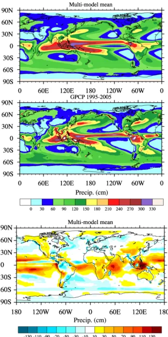
Fig. 5. Top: multi-model annual precipitation from the 2000 time slice experiment. Middle: annual
precipita-tion from GPCP. Bottom: difference (multi-model mean minus GPCP).
Fig. 5. Top: multi-model annual precipitation from the 2000 time
slice experiment. Middle: annual precipitation from GPCP. Bottom: difference (multi-model mean minus GPCP).
Model, also based on ECHAM5, but with differences in res-olution and shortwave radiation (Cagnazzo et al., 2007).
Some models used the previous AR4 simulations, ap-plying an approximate correspondence between RCPs and SRES scenarios (GEOSCCM, NCAR-CAM3.5; see Lamar-que et al., 2011). Finally, the CICERO-OsloCTM2 model used analysis data for year 2006 from ECMWF IFS analy-sis for all experiments.
Methane concentration (from Meinshausen et al., 2011, see Fig. 2) is prescribed at the surface (bottom layer or two layers, with or without a specified latitudinal gradient) in many models. It is prescribed over the whole atmosphere in CESM-CAM-Superfast and NCAR-CAM5.1 (using the NCAR-CAM3.5 distribution) and in STOC-HadAM3 and UM-CAM. Only LMDzORINCA uses methane emissions for historical and future simulations, while GISS-E2s use emissions only for future simulations. In both cases, those simulations include climate-dependent wetland emissions.
3.6 Photolysis
Photolysis rates in the models are computed with off-line (look-up table) or online methods. In the offline case, the look-up table contains values of photolysis rates for every photolytic reaction in the model over a range of pressures, solar zenith angles, overhead ozone columns and temper-atures. These pre-computed values are filled once at the start of the model run, and then interpolated at any time and grid point for the specific conditions in time and space. This method can be directly applied with a modulation to take into account local clouds and surface albedo (CESM-CAM-Superfast, CMAM, GFDL-AM3, LMDz-OR-INCA, MOCAGE, NCAR-CAM3.5 and NCAR-CAM5.1), while two models (HadGEM2, UM-CAM) do not apply such cor-rections. A drawback of this approach is the lack of coupling with the simulated aerosols.
Online photolysis schemes (CICERO-Oslo-CTM2,
EMAC, GEOSCCM, GISS-E2s, MIROC-CHEM and
STOC-HadAM3), solve the radiative transfer equation at each time-step and gridpoint, depending on local tempera-ture, pressure, aerosol content, cloudiness, surface albedo, overhead ozone column and solar zenith angle.
Note that a limited intercomparison of some stratospheric (and therefore of limited relevance to this study) photolysis rates is available in Chapter 6 of SPARC CCMVal (2010). Standard deviation on the order of 10–20 % are common for the major photolysis rates, although this could become larger in the troposphere due to interferences by clouds and aerosols.
3.7 Chemistry
3.7.1 Tropospheric gas-phase and aerosols
Apart from NCAR-CAM5.1 (which is aerosol-oriented with minimal chemistry; X. Liu et al., 2012), all models partic-ipating in ACCMIP simulate, at a minimum, gaseous tro-pospheric chemistry (Fig. 4). However, chemistry is repre-sented to various degrees of complexity: from 16 species in CESM-CAM-Superfast to 120 in GEOSCCM. This range is mostly due to the less or more detailed representation of non-methane hydrocarbon (NMHCs) chemistry (or lack thereof in the case of CMAM) for each model, with each having
Table 4. Globally-averaged mean bias and root-mean square
dif-ference for annual mean 700 hPa temperature (K) and precipitation (mm day−1). Note that because of their very similar climate diag-nostics, results from GISS-E2-R and GISS-E2-R-TOMAS are com-bined.
T 700 hPa (K) Precip (mm day−1)
Model Bias RMSD Bias RMSD
CESM-CAM-Superfast −0.06 0.94 0.19 1.25
CICERO 0.14 0.47 0.48 1.01
CMAM −0.10 1.14 0.28 1.41
EMAC −0.62 1.11 N/A N/A
GEOSSCM −0.77 1.22 0.17 1.11
GFDL-AM3 −1.40 1.71 0.31 1.34
GISS-E2-R(-TOMAS) −0.36 1.03 0.51 1.54
HadGEM2 −0.53 0.88 N/A N/A
LMDzORINCA N/A N/A N/A N/A
MIROC-CHEM −1.53 2.22 0.08 1.29
MOCAGE −0.99 1.48 −0.05 2.04
NCAR-CAM3.5 −1.03 1.33 0.10 1.34
NCAR-CAM5.1 N/A N/A N/A N/A
STOC-HadAM3 −1.41 1.74 0.28 1.13
UM-CAM −1.53 1.83 0.12 1.08
Multi-Model mean −0.78 0.91 0.22 0.98
its own lumping of NMHV emissions into species present in their chemical scheme. This is particularly important since it will automatically define the total amount of NMHC emis-sions released into the model atmosphere and NMHC re-activity as well as affect yields of radicals and intermedi-ate product species such as formaldehyde and glyoxal. In terms of NMHC chemistry, the smallest representations are in CESM-CAM-Superfast (where only isoprene is taken into account) and in HadGEM2 which does not include isoprene (only non-methane hydrocarbons up to propane are con-sidered). However, some simulations were also performed with HadGEM2-ExtTC (results of which are used only in Stevenson et al., 2012) which differ from HadGEM2 only by its extended chemistry scheme, including interactive bio-genic NMHCs. Only GEOSCCM, GISS-E2-R, MOCAGE
and CICERO-Oslo-CTM2 include the reaction of HO2with
NO to yield HNO3(Butkovskaya et al., 2007). Due to uncer-tainties on this reaction (Sander et al., 2011), it is important to identify which models include it as it significantly impacts the response of the tropospheric composition to changes in NOxemissions (Søvde et al., 2011).
NCAR-CAM5.1 and GISS-E2-R-TOMAS have the most extensive description of aerosols. Aerosols in NCAR-CAM5.1 are represented by three internally-mixed log-normal modes (Aitken, accumulation, and coarse), with the total number and mass of each component (sulfate, organic carbon, black carbon, mineral dust and sea salt) predicted for each mode (X. Liu et al., 2012). The TOMAS model alone has 108 size-resolved aerosol tracers plus three bulk aerosol-phase tracers. TOMAS predicts aerosol number and mass
5 hP
a
30 hP
a
200 hP
a
700 hP
a
Month
Month
Month
Month
cycle of temperature (K) at 4 pressure le v els for all models and the ERA-Interim reanalysis. 42
Fig. 6. Seasonal cycle of temperature (K) at 4 pressure levels for all models and the ERA-Interim reanalysis.
size distributions by computing total aerosol number (i.e. 0th moment) and mass (i.e. 1st moment) concentrations for each species (sulfate, sea salt, internally mixed elemental carbon, externally mixed elemental carbon, hydrophilic organic mat-ter, hydrophobic organic matmat-ter, mineral dust, aerosol-water) in 12-size bins ranging from 10 nm to 10 µm in dry diame-ter, following Lee and Adams (2011). The LMDzORINCA model simulates the distribution of anthropogenic aerosols such as sulfates, black carbon, particulate organic matter, as well as natural aerosols such as sea salt and dust. The aerosol code keeps track of both the number and the mass of aerosols using a modal approach to treat the size distribution, which is described by a superposition of log-normal modes (Schulz et al., 1998; Schulz, 2007). All other models that include aerosols use the bulk approach (i.e. computing mass only, with a specified distribution and no representation of coagu-lation).
Heterogeneous reactions on tropospheric aerosols are de-scribed through a limited set of heterogeneous reactions (5 or fewer), except GISS-E2-R-TOMAS, which has none.
The aerosol indirect effects are represented in approxi-mately half of the models (CICERO, GFDL-AM3, GISS-E2s, HadGEM2, MIROC-CHEM and NCAR-CAM5.1).
3.7.2 Stratospheric chemistry and ozone distribution
Many models have a full representation of stratospheric ozone chemistry (Fig. 4), with the inclusion of ozone-depleting substances (containing Br and Cl), and heteroge-neous chemistry on polar stratospheric clouds. For the mod-els without stratospheric chemistry, stratospheric ozone is specified in several ways. CESM-CAM-Superfast uses a lin-earized ozone chemistry parameterization (LINOZ, McLin-den et al., 2000). CICERO-Oslo-CTM2 uses monthly model climatological values of ozone and nitrogen species, ex-cept in the 3 lowermost layers in the stratosphere (approx-imately 2.5 km) where the tropospheric chemistry scheme is applied to account for photochemical O3 production in the lower stratosphere due to the presence of NOx, CO and NMHCs (Skeie et al., 2011b). Had-GEM2s, STOC-HadAM3 and UM-CAM input their time-varying stratospheric ozone
Global Tropics NH Extratropics SH Extratropics 400 hP a 400 hP a 700 hP a 700 hP a Month Month
Fig. 7. Seasonal cycle of specific humidity (g/kg); reanalysis data are from the ERA-Interim and AIRS are satellite retrievals (see text for details).
43
Fig. 7. Seasonal cycle of specific humidity (g kg−1); reanalysis data are from the ERA-Interim and AIRS are satellite retrievals (see text for
details).
distribution from the CMIP5 database (Cionni et al., 2011). Finally, LMDzORINCA uses a constant (for all simulations) climatological values of stratospheric ozone (Li and Shine, 1995). Note that changes in stratospheric ozone do affect photolysis in all other models but HadGEM2 and UM-CAM.
3.8 Radiation coupling
The composition-radiation coupling will depend on the sim-ulated species. Most of the CCMs use their simsim-ulated dis-tribution of water vapour and ozone to compute their di-rect radiative impact, except for HadGEM2 in which the online coupling is only applied in the troposphere, UM-CAM which is forced by offline data, and LMDzOR-INCA which has no ozone coupling. The simulated methane distribution is used for radiation calculations in EMAC,
GEOSCCM, HadGEM2, GISS-E2s, MIROC-CHEM and NCAR-CAM3.5. When aerosols are prognostically calcu-lated in the model (note that CESM-CAM-Superfast only simulates sulphate), they are all coupled to the radiation scheme. GEOSCCM and EMAC do not have an explicit aerosol description but they include in their computation of atmospheric heating profiles the radiative effect of aerosols taken from time-varying climatologies.
4 Evaluation of present-day climate
We present in this section an analysis and evaluation of se-lected climate diagnostics in the ACCMIP models. We focus on quantities that are directly relevant to chemistry modeling, namely precipitation, temperature, humidity and zonal wind.
41 Figure 8. Global annual mean precipitation change since 1850. The multi-‐model mean is indicated by the solid black dot, the median by the solid black line, the 25%-‐75% range by the extent of the colored box and the minimum/maximum by the extend of the whisker. Note the there is variation in the number of models between the various simulations (see Table 2). 2000 2100 2100 2100 2100 time slice -0.2 0.0 0.2 0.4 0.6 mm/day RCP2.6 RCP4.5 RCP6.0 RCP8.5
Fig. 8. Global annual mean precipitation change since 1850. The multi-model mean is indicated by the solid black dot, the median by the solid black line, the 25 %–75 % range by the extent of the colored box and the minimum/maximum by the extend of the whisker. Note the there is variation in the number of models between the various simulations (see Table 2).
44
Fig. 8. Global annual mean precipitation change since 1850. The
multi-model mean is indicated by the solid black dot, the median by the solid black line, the 25–75 % range by the extent of the colored box and the minimum/maximum by the extend of the whisker. Note the there is variation in the number of models between the various simulations (see Table 2).
In particular, temperature is analyzed at 700 hPa since that is representative of the main location of the tropical methane loss (Spivakovsky et al., 2000). Also, we only discuss annual means since our main interest is on long-term changes.
When compared against the Global Precipitation Clima-tology Project (GPCP) climaClima-tology for 1995–2005 (Adler et al., 2003), the simulated annual mean precipitation tends to be higher than observed over the tropical regions (ex-cept for tropical South America) in all models (Figs. 5 and S1). While the multi-model model annual mean precipita-tion (Fig. 5) provides many similarities to the CMIP3 multi-model mean in Randall et al. (2007; see their Fig. 8.5), there is also considerable improvement over Indonesia and the continental outflows of Asia and North America. Many models still suffer from an overestimate of the precipita-tion over the Indian Ocean and over high topography, the latter a consequence of the fairly coarse resolution used in these models. Overall, models tend to exhibit a positive area-weighted global mean bias (MB) against GPCP, ranging from 0.08 mm day−1(NCAR-CAM3.5) to 0.51 mm day−1 (GISS-E2-R) except for MOCAGE (−0.05 mm day−1), which also features a fairly large (> 1 mm day−1) area-weighted root mean square difference (RMSD) (see Table 4 and Fig. S1). This global positive bias in all models but MOCAGE will likely lead to an overestimate of the wet removal rate, espe-cially for soluble chemical species in the tropical regions. However, a recent analysis of satellite-based precipitation estimates (Stephens et al., 2012) indicates that the GPCP precipitation rates over the oceans could be underestimated by approximately 10 % or 0.3 mm day−1 over the tropical
42
Figure 9. Same as Figure 8 but for 700 hPa temperature change since 1850.
2000 2100 2100 2100 2100 time slice 0 2 4 6 8 K RCP2.6 RCP4.5 RCP6.0 RCP8.5
Fig. 9. Same as Fig. 8 but for 700 hPa temperature change since 1850.
45
Fig. 9. Same as Fig. 8 but for 700 hPa temperature change since
1850.
oceans and more over the extra-tropical oceans. This means that many of the models are possibly providing reasonable large-scale precipitation rates (regional biases are doubtless still present), which would considerably reduce the possible biases on wet removal rates.
Similarly for temperature (Fig. 11), in the case of RCP2.6, the simulated change in CESM-CAM-Superfast shows an outlying negative bias, and the warming trend for NCAR-CAM3.5 is lower than any other model. There is much more inter-model agreement with the RCP8.5, with CESM-CAM-Superfast being showing the lowest temperature increase. Such inter-model variations will have consequences (in par-ticular through the link of OH and specific humidity) for the interpretation of 21st-century trends, especially methane life-time. Indeed, as discussed in Voulgarakis et al. (2012), there is considerable spread in the estimated climate feedback on the methane lifetime (0.33±0.13 yr K−1). In the lower tropo-sphere (700 hPa, approximately 3 km, Table 4 and Fig. S2), the modeled temperatures tend to be biased cold compared to the European Centre for Medium-Range Weather Fore-cast Reanalysis Interim products (ERA-Interim, Dee et al., 2011; note that other reanalyses have very similar temper-ature distributions and therefore do not change the conclu-sions, not shown), with a MB ranging between −1.5 K and close to 0 K. At the global scale, the interannual variability in the ERA-Interim temperature at that pressure is on the or-der of 0.3 K, meaning that many of the biases are significant (Fig. 6). CICERO-OsloCTM2 used fixed 2006 meteorology and therefore exhibits little difference with the climatology used for evaluation. The RMSD is larger than 1 K in all mod-els. This negative bias is even more pronounced in the upper-troposphere and lower-stratosphere (200 hPa, Figs. 6 and S3), with biases as high as 6 K in all regions. Only CMAM has
43
Figure 10a. Difference 2000-‐1850 in annual and zonal mean specific humidity (10-‐6 kg/kg).
Fig. 10a. Difference 2000–1850 in annual and zonal mean specific humidity (10
Fig. 10a. Difference 2000–1850 in annual and zonal mean specific humidity (10 −6kg kg
−1).
−6kg kg−1).
a slight positive bias (1–2 K) in the tropical regions (Fig. 6). The temperatures biases are however smaller closer to the surface (see the 850 hPa level in Fig. 6).
Specific humidity (using as references the ERA-Interim reanalysis and the Atmospheric InfraRed Sounder retrievals, AIRS, Divarkta et al., 2006) biases somewhat reflect the tem-perature biases (as illustrated by C. Liu et al., 2012), gener-ally showing negative differences (Fig. S4), with a clear neg-ative bias in the tropical regions in the troposphere for many models, associated with the aforementioned bias in the tropi-cal precipitation. Many models also tend to exhibit a positive bias in specific humidity in the mid-troposphere (400 hPa,
Fig. 7), especially when compared to AIRS. Biases in spe-cific humidity in the tropical mid-troposphere will directly translate in biases in OH, since (O1D + H2O) is the primary source of OH in that region. The impact on ozone is however of variable sign depending on the chemical conditions (Jacob and Winner, 2009).
The position of the polar jet is important as it defines the extent of the polar vortex in which ozone depletion may oc-cur. Many models tend to overestimate the strength of the Southern Hemisphere polar jet by 10–20 m s−1 compared to ERA-Interim (Fig. S5). This is also true of the North-ern Hemisphere polar jet, but to a lesser extent. EMAC and
44
Figure 10b. Difference 2100-‐2000 in annual and zonal mean specific humidity (10-‐6 kg/kg)
for RCP2.6. The CESM-‐CAM-‐superfast results are spurious because of a mismatch in the
SSTs used (see text for details).
Fig. 10b. Difference 2100–2000 in annual and zonal mean specific humidity (10
−6kg kg
−1) for RCP2.6.The
CESM-CAM-superfast results are spurious because of a mismatch in the SSTs used (see text for details).
Fig. 10b. Difference 2100–2000 in annual and zonal mean specific humidity (10−6kg kg−1) for RCP2.6. The CESM-CAM-Superfast results
are spurious because of a mismatch in the SSTs used (see text for details).
GISS-E2s tend to show a negative bias in those regions. The biases in the Southern Hemisphere polar zonal wind dis-tribution are strongly anti-correlated with the temperature biases in the same region (see Figs. S3 and S5); for
ex-ample, CESM-CEM-Superfast poleward of 60◦S and above
100 hPa. In the tropical lower stratosphere, there is a mixture of strong positive and negative biases, along with relatively small biases.
The mid-latitude jets are important as they define the ex-tent of the tropical regions. Most models exhibit minor bi-ases, although the CMAM and GISS-E2s models clearly overestimate its strength.
5 Climate change as simulated in ACCMIP
In this section, we document the simulated annual-mean changes in climate, over the simulated historical (1850– 2000) and future (2000–2100) periods, emphasizing RCP2.6 and RCP8.5 for the latter since they represent the extremes of projected 2100 climate change under the RCPs. Results from CICERO-OsloCTM2 are ignored since they used the same meteorological fields for all time slices. The purpose of this section is to inter-compare model simulations to identify potential outliers.