HAL Id: hal-02923809
https://hal.archives-ouvertes.fr/hal-02923809
Submitted on 17 Sep 2020
HAL is a multi-disciplinary open access
archive for the deposit and dissemination of
sci-entific research documents, whether they are
pub-lished or not. The documents may come from
teaching and research institutions in France or
abroad, or from public or private research centers.
L’archive ouverte pluridisciplinaire HAL, est
destinée au dépôt et à la diffusion de documents
scientifiques de niveau recherche, publiés ou non,
émanant des établissements d’enseignement et de
recherche français ou étrangers, des laboratoires
publics ou privés.
A three-dimensional synthesis study of δ 18 O in
atmospheric CO 2 : 2. Simulations with the TM2
transport model
Philippe Ciais, Pieter Tans, A. Scott Denning, Roger Francey, Michael Trolier,
Harro Meijer, James White, Joseph Berry, David Randall, G. James Collatz,
et al.
To cite this version:
Philippe Ciais, Pieter Tans, A. Scott Denning, Roger Francey, Michael Trolier, et al.. A
three-dimensional synthesis study of δ 18 O in atmospheric CO 2 : 2. Simulations with the TM2 transport
model. Journal of Geophysical Research: Atmospheres, American Geophysical Union, 1997, 102 (D5),
pp.5873-5883. �10.1029/96JD02361�. �hal-02923809�
JOURNAL OF GEOPHYSICAL RESEARCH, VOL. 102, NO. D5, PAGES 5873-5883, MARCH 20, 1997
A three-dimensional
synthesis
study
of
in atmospheric
CO
2
2. Simulations with the TM2 transport model
Philippe Ciais,
• Pieter P. Tans,
2 A. Scott Denning,
3 Roger J. Francey,
4
Michael Trolier? Harro A. J. Meijer, 6 James W. C. White?
Joseph
A. Berry,
7 David A. Randall,
3 G. James Collatz,
8
Piers J. Sellers,
8 Patrick Monfray, 9 and Martin Heimann •0
Abstract. In this study, using a three-dimensional
(3-D) tracer modeling approach,
we
simulate
the •80 of atmospheric
CO2.
In the atmospheric
transport
model
TM2 we
prescribe
the surface
fluxes
of •80 due to vegetation
and soils,
ocean
exchange,
fossil
emissions, and biomass burning. The model simulations are first discussed for each reservoir separately, then all the reservoirs are combined to allow a comparison with the
atmospheric
•80 measurements
made
by the National
Oceanic
and
Atmospheric
Administration-University of Colorado, Scripps Institution of Oceanography-Centrum
Voor Isotopen Onderzoek (United States-Netherlands)
and Commonwealth
Scientific
and
Industrial Research
Organisation
(Australia) air sampling
programs.
Insights
into the
latitudinal
differences
and into the seasonal
cycle
of •80 in CO2 are gained
by looking
at
the contribution of each source. The isotopic exchange with soils induces a large isotopic depletion over the northern hemisphere continents, which overcomes the concurrent effect of isotopic enrichment due to leaf exchange. Compared to the land biota, the ocean fluxes and the anthropogenic CO2 source have a relatively minor influence. The shape of the
latitudinal
profile
in •80 appears
determined
primarily
by the respiration
of the land
biota, which balances photosynthetic uptake over the course of a year. Additional information on the phasing of the terrestrial carbon exchange comes from the seasonal
cycle
of •80 at high
northern
latitudes.
1. Introduction
The oxygen isotope composition of atmospheric CO2 may yield new insight on how the terrestrial biosphere absorbs and respires CO2. Of primary importance is the fact that CO2 exchanges isotopically with water, according to an isotopic reaction that is catalyzed by the enzyme carbonic anhydrase. Francey and Tans [1987] and Farquhar et al. [1993] have further quantified the importance of the vegetation and soils and shown that /5180 in CO2 is linked to the gross biospheric carbon fluxes. Both the photosynthetic assimilation uptake and
•Laboratoire de Modfilisation du Climat et de l'Environnement,
Commissariat h l'Energie Atomique l'Orme des Merisiers, Gif sur
Yvette, France.
2Climate Monitoring and Diagnostic Laboratory, NOAA, Boulder, Colorado.
3Department of Atmospheric Sciences, Colorado State University, Fort Collins.
4Division of Atmospheric Research, Commonwealth Scientific and
Industrial Research Organisation, Melbourne, Victoria, Australia.
5Institute of Arctic and Alpine Research and Department of Geo-
logical Sciences, University of Colorado, Boulder.
6Centrum voor Isotopen Onderzoek, University of Groningen, Gro-
ningen, Netherlands.
7Department of Plant Biology, Carnegie Institution of Washington, Stanford, California.
8NASA Goddard Space Flight Center, Greenbelt, Maryland.
9Centre des Faibles Radioactivit•s, Laboratoire de Mod•lisation du
Climat et de l'Environnement, Gif sur Yvette, France.
mMax-Planck-Institut fiir Meteorologie, Hamburg, Germany.
Copyright 1997 by the American Geophysical Union.
Paper number 96JD02361.
0148-0227/97/96JB-02361509.00
the total ecosystem
respiration
release
drive
the (•180
in CO2.
In a companion paper [Ciais et al., this issue] (hereinafter referred to as part 1) we have presented a detailed calculation
of the surface
fluxes
that control
(5180
in CO2. In the present
study we prescribe these surface fluxes into a three-dimen- sional (3-D) model of atmospheric transport, the TM2 model [Heimann and Keeling, 1989; Heimann, 1995], in order to cal-
culate
the atmospheric
(5180
in CO2 on a 7.5
ø horizontal
grid
every 3 hours.
The modeled (5180 field results from exchange with five different reservoirs. Before comparing the simulated (5180 with observations, we examine separately the contribution of each reservoir in order to identify the dominant mechanisms. The model results are then discussed together with atmospheric measurements at specific locations around the world. We give
special
attention
to the latitudinal
profile of (5180
which is
characterized by a pronounced isotopic depletion in the north- ern hemisphere with respect to the southern hemisphere. Also, we examine the seasonal cycle of (5180 at three sites where the observational record is particularly well documented: Point Barrow (71øN), Mauna Loa (20øN), and Cape Grim (41%).
The atmospheric observations are from flask samples col- lected at remote marine boundary layer sites. These measure- ments come from three independent air sampling networks: the National Oceanic and Atmospheric Administration- University of Colorado (NOAA-CU) network of 17 sites ana-
lyzed
for 180 during
1990-1994
(M. Trotier et at., An evalua-
tion of the effects of oxygen exchange on (5180 measurements from NOAA Global Air Sampling Network, submitted to Global Biogeochemical Cycles, 1996) (hereinafter referred to as Trotier et at., submitted manuscript, 1996), the Scripps Insti- 5873
5874 CIAIS ET AL.: STUDY OF A180 IN ATMOSPHERIC CO2, 2
tution of Oceanography-Centrum voor Isotopen Onderzoek (Scripps-CIO) network of 10 sites measured between 1977 and 1992 (H. A. Meijer et al., manuscript in preparation, 1996), and the Commonwealth Scientific and Industrial Research Or- ganisation (CSIRO) network from which we used two sites at high southern latitudes [Francey and Tans, 1987; Francey et al., 1990, 1995]. All three experimental groups have independent sampling strategies and calibration procedures. For instance, the CSIRO group dries the air when sampling, which ensures no isotopic reaction of CO2 and water within the flask. Nev-
ertheless,
no systematic
correction
was applied
to the 8180
data from each different group when merging the three data sets. In this paper, sinks correspond to a negative net flux of carbon (CO2 is removed from the atmosphere) and sources correspond to a positive net flux (CO2 is released to the atmo- sphere). Isotopic ratios are expressed in per mil (%0), defined as
8180
-'-
1000
I (180/16Oh
!sample (18(•/16(•h ß --t -- ( '-'! standard180/160)
standardFor CO2, all isotopic values are given relative to the stan- dard isotopic ratio Vienna Pee Dee belemnite (VPDB)-CO2 = 0.002088349077 as recommended by Allison et al. [1995]. For H20 we express isotopic abundance relative to the standard Vienna SMOW (VSMOW) = 0.00200520 [Baertchi and Mack- lin, 1965]. We must subtract +41.47%o to express VSMOW
values in the VPDB-CO2 scale. This includes a difference
equivalent to -30.9%0 between VSMOW and VPDB-calcite and accounts for the 180 fractionation during CO2 evolution at 25øC with 100% phosphoric acid [Friedman and O'Neill, 1977] between VPDB-calcite and VPDB-CO2.
2. Atmospheric Measurements From Three Air
Sampling Programs
2.1. NOAA-CU Data
Since 1990, the Institute for Arctic and Alpine Research at
the University
of Colorado
(CU) has
been
measuring
the •3C/
•2C and •80/•60 isotope
ratios
of atmospheric
CO2 in flask
samples of air provided by the NOAA Global Air Sampling Network. The sampling strategy and techniques (as relevant to CO2 monitoring) have been described by Conway et al. [1994], while the analytical methods and calibration of the isotope data have been presented by Trolier et al. [1996]. The features
of the sampling
methodology
most
relevant
to the 8•80 data
are that flasks are collected in pairs as a check on sample quality and that to date, almost all the NOAA samples have been collected without drying the air prior to storage in the glass flasks. Thus, while the NOAA-CU data from high- latitude sites appear to faithfully record the 8•sO of atmo- spheric CO2, measurements from flasks filled at more humid sampling sites are obviously contaminated, showing greatly increased differences between the two members of a pair and unrealistically rapid fluctuations. These effects have been at- tributed to exchange of oxygen between CO2 and water con- densed on the flasks wall [Gemery et al., 1996]. Trolier et al. (submitted manuscript, 1996) have used the statistical proper-
ties of the 8•80 data, supplemented
by comparisons
of "wet"
and recently
available
"dry"
8•O data
at two sites
(Samoa
and
Cape Kumukahi), to evaluate which of the NOAA sites pro- vide 8•80 data that is representative of the true atmospheric signatures.
2.2. Scripps-CIO Data
The cooperation between Scripps Institution for Oceanog- raphy and CIO (Centrum voor Isotopen Onderzoek) started in 1977. From then on, the samples from the older Scripps net- work for CO2 concentration monitoring were also isotopically analyzed at CIO in Groningen, Netherlands, starting with five stations (La Jolla, Mauna Loa, Cape Kumukahi, Fanning Is- land, and South Pole [Mook et al., 1983]), later extended over the whole Scripps monitoring network (see Keeling et al. [1989],
who only
report
13C
measurements).
The sample
handling,
as
well as the results of the first years of monitoring, are described by Mook et al. [1983]. Flask samples were taken without drying, shipped to Scripps, and analyzed for the CO2 concentration. Then, CO2 was extracted cryogenically and shipped to CIO, first in cork-stopped flasks, later in flame-off tubes.
At CIO the samples were measured on an (IRMS) machine, in the early years on a modified MM 903, later on a SIRA 9. All
samples
have
been
analyzed
both for 13C
and 180. The results
were corrected for the influence of N20 [Mook and Jongsma, 1987]. Calibration was maintained on the basis of NBS19 car- bonate, both for 13C and 180. The latter scale was comain- tained by using VSMOW water as reference material and checking continuously for the reproducibility of the known difference between these two primary reference materials. This
has proven
to be of utmost
importance,
since
unlike
for 13C,
the preparation
route for 180 involves
large
fractionation
fac-
tors (and thus possibilities for errors). Throughout the years, several local reference materials have been used for the main- tenance and checking of the calibration: carbonates, waters, and pure CO2 standards. An extensive "history recalibration" exercise has been carried out based on multiple variable least squares techniques to reestablish the calibration of the mass spectrometers over the years, based on all the calibration mea- surements of primary and local standards (H. Roeloffzen, un- published data, 1996). Final errors (random and calibration) are estimated to be +_0.025%0 for 818C and +_0.06%0 for 8180, with the exception of the first several years, in which the errors
were larger.
The Scripps sampling procedure did not involve drying. Al-
though
this could
influence
the 8180 values,
the overview
of
the isotopic data shows that this has not happened (perhaps apart from isolated clear "outliers"). The isotopic measure- ments on the Scripps network by CIO were terminated in 1992. From then on, isotopic measurements were carried out at Scripps itself. A full report on the Scripps-CIO data is underway. 2.3. CSIRO Data
Francey and Tans [1987] used data from five and six sites from the CSIRO global network for 1984 and 1985, respec- tively, and results through 1988 are presented by Francey et al. [1990]. Typically, 12-15 sites have been routinely sampled since the late 1980s by CSIRO. While precision is relatively high, particularly in low-latitude sites (as a result of drying all samples on collection), systematic errors are apparent in the data which are still under investigation. For this reason, only selected data from the original sites are used here. Of partic- ular relevance is the Cape Grim in situ record, unique for the cryogenic removal of water and extraction of CO2 on collection [Francey et al., 1995]. The Cape Grim record provides a long high-precision time series permitting good definition of the small seasonality in the southern hemisphere.
CIAIS ET AL.: STUDY OF A•80 IN ATMOSPHERIC CO2, 2 5875
3. TM2 Transport Model
We coupled
the surface
fluxes
of C•8OO and CO2 with the
atmospheric tracer model TM2 in order to simulate the global distribution of 8280 in atmospheric CO2. The TM model fam- ily was developed at the Max Planck Institute (Hamburg, Ger- many) and described by Helmann and Keeling [1989] for TM1 and by Helmann [1995] for TM2. The model grid is 7.5 ø by 7.5 ø in the horizontal, with nine vertical sigma levels and a time step of 3 hours. The horizontal mass fluxes are prescribed from the analysis of meteorological wind fields at the European Centre for Medium-Range Weather Forecasting (ECMWF) every 12 hours. The large-scale vertical mass fluxes are derived from mass continuity. Sub-grid-scale vertical transport due to both penetrative and shallow cumulus convection are calculated at each time step following the scheme of Tiedke [1989], together with vertical diffusion [Louis, 1979]. Specifically, the intensity of convective upward motion is calculated using the moisture budget at the cloud base, determined by the transported sur- face evaporation fluxes. The model does not have a realistic description of the stable boundary layer, which may bias the simulated surface concentrations, especially over the conti- nents [Denning et al., 1995]. For this reason, we do not consider diurnal variations in the surface fluxes.
The boundary conditions of the model are monthly fluxes of tracer averaged onto the model's grid. We verified that chang- ing the grid of the surface fluxes conserved the total mass of tracer emitted to the atmosphere. Starting with an initial con- centration field equal to zero everywhere in the atmosphere, we spun up the transport model by running the fluxes repeat- edly during three model years with the atmospheric transport of 1990, then archived the simulated fourth year with the 1990
transport.
For each
reservoir
the species
CO2 and C18OO
are
run separately,
and the corresponding
8180 distribution
is cal-
culated off-line after transport. Starting with tracer concentra- tions of zero at the beginning of the spin up, we add an arbitrary atmospheric "baseline" concentration Ccst to the sim- ulated field of concentrations (see section 4.5). We thus have expressed all 8180 fields in the atmosphere relative to the
observed annual mean value of +0.85%0 at South Pole station.
4. Simulated
•80 in COz
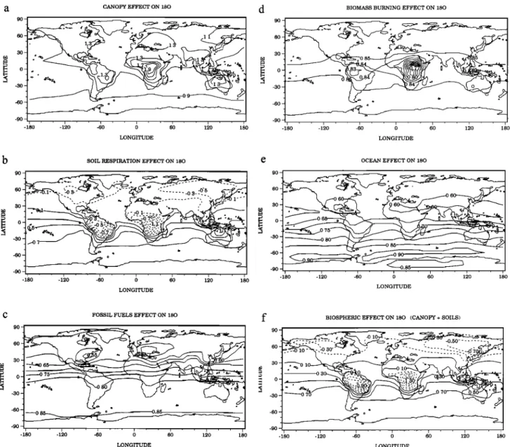
4.1. The •80 Resulting From Isotopic Exchange in Leaves Figure la shows the simulated 8180 of atmospheric CO2 at the lowest model level resulting from canopy isotopic ex- change. There is an Arctic minus Antarctic difference of +0.3%0, because the zonally averaged 8•80 value of CO2 in leaves is greater than the atmospheric value in the northern hemisphere, except north of about 60øN (part 1, Plate 2). This confirms previous results of Francey and Tans [1987] and Far- quhar et al. [1993, Figure 4] in which atmospheric mixing pro- cesses were not included. The isotopic exchange with leaves has the largest influence on atmospheric 8180 over very pro- ductive source regions, especially over tropical and temperate forest ecosystems. Conversely, areas of low productivity and deserts have an almost negligible imprint on the atmospheric 8180, a striking example being the fact that the broad maxi- mum of 8180 in leaf CO2 at 30øN over the Sahara and the
Middle East (Plate 2c of part 1) does
not appear
in the 8180
distribution of Figure la.
There are two distinct maxima in 8180 over Brazil and equa- torial Africa, with values locally 1%o above the zonal average.
Similarly, there is a broad, although less pronounced maximum in 8180 over Europe and North America. Francey and Tans
[1987] suggested
that low 8•80 values
measured
at Barrow
(Alaska, 75øN) might be related to the isotopic exchange in leaves, but they also pointed out the need for an additional source of depleted CO2 such as soils. In our simulation, CO2
over Europe
and eastern
Siberia
is more depleted
in 180 due
to canopy exchange than Europe and western Siberia. On the other hand, Figure la confirms that the mechanism of leaf isotopic exchange cannot account for the observed gradient of
about -1%o between Alaska and Hawaii. This is mainly the
result of lower productivity at the highest latitudes (where canopy 8•80 is lowest) relative to that of the temperate zone. 4.2. The •180 Resulting From Soil Exchange
Figure lb shows
the simulated
atmospheric
8180 surface
values resulting from soil exchange. There is a -1.2%o differ- ence between the Arctic and the Antarctic. The latitudinal profile has a two-step shape, with one decrease between 30øS and the equator and another from 30øN to 60øN. We obtain a
minimum in 8180 over Siberia and over North America be-
cause CO2 emitted by soils is isotopically depleted (Plate lb of
part 1). There are also two pronounced
minima
in 8180 of
atmospheric CO2 over South America and Africa, both areas being characterized by a huge respiratory efflux of CO2 that is moderately depleted in 180 with respect to the atmosphere. However, it is possible that our model underestimates the 8180 value of CO2 over tropical land areas because the 8180 of meteoric water that we use may be 1-2%o lower than in the real world, based on the International Atomic Energy Agency (IAEA) measurements in precipitation in Brazil and Zimba- bwe [IAEA, 1981;Jouzel e! al., 1987]. There is a sharp minimum in 8180 respired by soils over equatorial Africa, in the same
spot
characterized
by a peak in leaf 8180,
which
is due primar-
ily to very high productivity in this grid cell.
4.3. The •i•80 Resulting From the Combustion of Fossil
Fuels and From Tropical Biomass
Figure
lc shows
the 8•80 in atmospheric
CO2 caused
by the
burning of fossil fuels. Fossil fuel emissions deplete the north- ern hemisphere air in 180 by 0.3%0 with respect to the south- ern hemisphere, because of relatively slow interhemispheric transport. The 8180 decrease from south to north in Figure lc mirrors higher concentrations of fossil CO2 over Europe and North America. The simulated north minus south difference in fossil CO2 is about 5 ppm. Similarly, Figure l c shows that the 8180 minima over Europe and North America correspond to maximum emissions of fossil CO2 over industrialized regions.
Figure ld displays the influence exerted by biomass burning emissions of CO2 on 8180 at the ground level. As expected, we model local minima in 8180 of up to 0.1%o below the zonal average over tropical regions which undergo intense biomass burning: equatorial Africa, the Amazon basin, and SE Asia. However, the isotopic depletion due to biomass burning is confined over the source regions, and the zonally averaged variation in 8180 indicates only a -0.02%o minimum around the equator. This is only a minor effect compared to fossil fuel emissions which cause a zonal mean depletion of 0.3%0 in the northern hemisphere (Figure l d). Despite the fact that bio- mass burning adds 283 Tmol of CO2 per year (3.3 GTC) to the
atmospheric
burden
compared
to 500 Tmol yr -1 (6 GTC) for
fossil emissions, its impact on surface 8180 values is diminished because strong vertical transport in the tropics prevents the
5876 CIAIS ET AL.: STUDY OF A180 IN ATMOSPHERIC CO2, 2 CANOPY EFFECT ON 180 60- -30 - -60 - -90 -
d BIOMASS BURNING EFFECT ON 180
-180 -1•0 -•0 ; 6; 140 180 -180 -1•0 -•0 ; 610 140 180 90 60 3O
o
-30 - -6O - -90 - LONGITUDE LONGITUDE SOIL RESPIRATION EFFECT ON 180.- -0.1 ... k ' : ; 610 140 180 LONGITUDE e OCEAN EFFECT ON 180 ß • 0.6 I
-180
-1•0
-•0
-180
-1•0
-60I
0
61o •0 •80 LONGITUDE 90 60 3O -30 -60 -90FOSSIL FUELS EFFECT ON 180 f BIOSPHERIC EFFECT ON 180 (CANOPY + SOILS)
_
-la0 -120 -60 0 6; 120 ' 180 ' -180 ' -1•0 -•0 ; 610 1•0 180
LONGITUDE LONGITUDE
Figure 1. Annual mean r5180 in CO2 at the surface level, after transport of the surface sources by the
transport
model
TM2. (a) The r5180
resulting
from leaf exchange.
(b) The r5•80
resulting
from soil
respiration.
(c) The r5180
resulting
from fossil
fuel emissions.
(d) The r5•80
resulting
from air-sea
exchange.
(e) The r5•80
resulting
from biomass
burning
emissions.
(f) "Biospheric"
r5180,
combination
of leaf exchange
and soil
respiration. All fields are plotted relative to the observed South Pole station annual mean value of +0.85%0.
CO2 emitted by fires to build up at the surface level. In other words, the tropical biomass burning source is diluted in the ver-
tical, whereas the fossil source is more confined near the surface.
4.4. The •i•80 Resulting From Ocean Isotopic Exchange Figure le shows the simulated r5180 in atmospheric CO2 at the surface as resulting from ocean exchange. There is a per- manent negative difference in r5180 of -0.3%0 between the north and the south, the largest decrease taking place between approximately 40øS and 10øN. This latitudinal difference can be compared with Plate 3b of part 1, representing r5180 of CO2 dissolved in the ocean. Although high-latitude oceans in both hemispheres are enriched in 180 to similar magnitudes, there is a much greater ocean area in the south, which likely causes the decrease in r5180 from south to north apparent in Figure le. Additionally, the air-sea gas exchange in the southern ocean is more vigorous than over the northern oceans [Erickson, 1993].
Locally, at around 60øS, stronger winds enhance the transfer
of enriched CO2 dissolved in surface waters to the atmosphere,
yielding
maximum
values
in r5180
which
decrease
farther
to the
south, over Antarctica. There is little longitudinal variation in r5•80 resulting from ocean exchange. However, Figure le in- dicates two "tongues" of northern hemisphere air depleted in •80 over South America and Africa, the passage of northern hemisphere air across the equator being facilitated over the
tropical
continents,
as previously
noticed
in 8SKr
simulations
with the TM1 model by Heimann and Keeling [1989] (the TM2
model
is close
to TM1 for 8SKr).
4.5. Combined •180 Fields
The atmospheric "total" r5180, corresponding to exchange with all reservoirs, r5 a, is obtained from the combination of the concentration fields due to each separate reservoir. In every
CIAIS ET AL.' STUDY OF A180 IN ATMOSPHERIC CO2, 2 5877
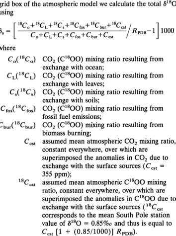
grid box of the atmospheric
model
we calculate
the total 8•80
using
i18Co
-'[- CL -[- Cs -[- C fos18 18 18 18 18
-[- Cbur -[- Ccst /where
Co(•8Co) CO2 (C•8OO) mixing
ratio resulting
from
exchange with ocean;
CL(•aCL) CO2 (C•8OO)
mixing
ratio resulting
from
exchange with leaves;
Cs(•8Cs) CO2 (C•8OO)
mixing
ratio resulting
from
exchange with soils;
Cfos(laCfos)
CO 2 (C•8OO) mixing
ratio resulting
from
fossil fuel emissions;
Cbur(•aCbur)
CO2 (C•8OO)
mixing
ratio resulting
from
biomass burning;
Ccst assumed mean atmospheric CO2 mixing ratio, constant everywhere, over which are
superimposed the anomalies in CO2 due to exchange with the surface sources (Cc•t = 355 ppm);
18Ccs
t assumed
mean
atmospheric
C•8OO mixing
ratio, constant everywhere, over which are
superimposed
the anomalies
in C•8OO due to
exchange
with the surface
sources
( • 8Cc•
t
corresponds to the mean South Pole station value of/3•80 = 0.85%0 and thus is equal to Ccs t [1 + (0.85/1000)] RpDB).
4.6. Combination of Vegetation and Soils (Biospheric 8•SO) Figure if shows the /3•80 resulting from soil and leaf ex- change combined, all other sources being set to zero in the equation given in section 4.5. While leaves and soils separately
generate
north
minus
south
differences
in atmospheric/3•80
of
similar amplitude but opposite in sign (Figures la and lb), the superposition of both yields a net negative north minus south
latitudinal
difference
of -0.9%0. The biospheric/3•80
at the
surface level has two main regional minima, corresponding to an isotopic depletion of the atmospheric reservoir: one over the eastern part of Siberia and another over the Amazon. Over
these
areas
the exchange
with the land biota determines/3•80
values that are typically 0.6%0 below the zonal average. Despite the fact that the annual mean uptake of CO2 by canopy photosynthesis (,4) is locally equal to the release of CO2 by respiration (•), the soil source has a larger influence on the atmospheric/3•80 because CO2 in soils bears a larger isotopic disequilibrium with respect to the atmosphere than CO2 in leaves (compare Plates lb and 2c of part 1). Another factor which contributes an additional asymmetry between the vegetation and the soils is the fact that the atmospheric circu-
lation
tends
to accumulate
some
CO2 issued
from soil
respi-
ration over continental Asia due to seasonal differences in the vertical and southward transport intensity [Keeling et al., 1989;
Denning
et al., 1995].
Since
CO2 from soils
has a lower/3•80
value than CO2 from leaves, this pattern of the northern hemi-
sphere
circulation
decreases
the/3•80 in the atmosphere
over
Siberia due to the accumulation of respired CO2 near the surface over that region (Figure if).
4.7. Combination of All Reservoirs
The •80 in atmospheric CO2 in the lowest model layer resulting from exchange with all reservoirs is shown in Figure
2. Comparison of Figure 2 with Figure l c shows that the total /3•80 is dominated by terrestrial processes. There is a decrease in/3•80 from south to north of 1.5%o, mostly contributed by soils and to a lesser extent by fossil CO2. There are also im- portant longitudinal variations characterized by large negative anomalies in/3•80 over the continents, which are due to soil respired CO2. In the latitude band around 65øN, we simulate
an east-west difference of -0.6%0 in/3•80 between Siberia and
the North Atlantic. Around the equator, we obtain two pro-
nounced/3•80 minima both over the Amazon basin and over
Equatorial Africa, with an additional decrease in atmospheric /3•80 over SE Asia. Such large longitudinal differences in the simulated/3•80 fields have no equivalent in the CO2 distribu- tion because the isotopic exchange with the biosphere is more vigorous than for CO2, due to the isotopic disequilibrium fluxes (part 1).
5. Comparison
With •80 Measurements
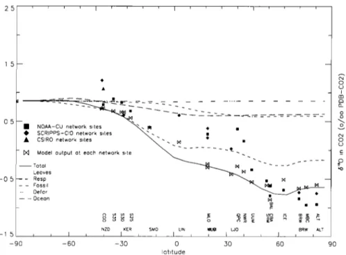
5.1. North Minus South Differences in 8180Figure
3 compares
the zonally
averaged
simulated
•80 field
with the NOAA-CU, Scripps-CIO, and CSIRO observations, all zonal profiles being referenced relative to the value of
+0.85%0
at the South
Pole (the observed
average
•80 mea-
sured by CSIRO at the station in 1990). We simulate a de- crease in total •80 from south to north of -1.5%o, compa- rable in magnitude to the observed pattern. There are two
steps
on the simulated
average
•80: a first drop of -1%o
between 40øS and the equator, and a smoother decrease of -0.5%0 between 0 and 60øN. North of 60øN, •80 slightly increases by 0.1%o.
The atmospheric measurements also suggest a two-step de- crease from south to north, although all tropical sites are measured without drying the air, which gives us less confidence in the measured •80. Yet the model fails to predict high enough •80 values between 0 and 40øN. As an example, at Fanning Island (3øN, Scripps-CIO site LIN in Figure 3), Mauna Loa (19.5øN, NOAA-CU and Scripps-CIO site MLO in Figure 3), and La Jolla (32.9øN Scripps-CIO site LJO in Figure
3), our calculations
underestimate
•80 by roughly
0.5%0.
A
second discrepancy between model and observations exists at
high northern
latitudes,
where
the simulated
•80 values
are
0.2%0 above the observations. The data indicate a markeddrop in •80 of about -1%o between La Jolla and Barrow,
whereas we model a decrease of less than -0.5%0. In the
southern
tropics
we slightly
underestimate
the •80 compared
to the measurements on the NOAA-CU ship cruises (sites S35 to S25 on Figure 3), but this needs to be confirmed by mea- surements made on dry air samples.
Figure 3 indicates that the •80 obtained in the model at Fanning Island (3øN, Scripps-CIO site denoted LIN in Figure 3) is 0.3%0 above the calculated zonal mean value at this
latitude. This model feature is due to minima in •80 over
equatorial Africa and Brazil (Figure 2) which make the zonal
mean •80 lower than the value calculated at a remote mari-
time site. This raises a cautionary flag about the zonal repre- sentativeness of the existing marine boundary layer stations
where
•80 is routinely
measured.
Similarly,
strong
•80 dif-
ferences between ocean and continent at high northern lati-
tudes
may explain
why •80 is higher
at Iceland
(20øW;
63øN
denoted ICE in Figure 3) than at Cold Bay (163øW; 55øN denoted CBA) and at Barrow (156øW; 71øN denoted BRW),
5878 CIAIS ET AL.' STUDY OF A•80 IN ATMOSPHERIC CO2, 2
60 '" --- ø • '" -0.0 •-_.l.._,,--
a01_7___0.a
....
.... '---i
....
-0.a.__
-80
.
I I ' ' I ' ' I ' ' [ ' ' I '
-180 -120 -60 0 60 120 180
LONGITUDE
Figure
2. Annual
mean
8180
in CO2
at the surface
level
resulting
of terrestrial
fluxes,
air-sea
exchange,
and
anthropogenic CO2 emissions (combination of all reservoirs).
both in the model and on the NOAA-CU and Scripps-CIO observations (Figure 3).
A better understanding of the discrepancies between this standard experiment and the 8•80 measured at the stations will require a full study of the sensitivity of our model to its prescribed parameters. One can distinguish two types of pa- rameters, related on one hand to the isotopic hydrology (i.e.,
8•80 of H20 in leaves
and soils)
and on the other
hand
to the
biospheric carbon fluxes (i.e., assimilation A and total respira-
tion 3t). A detailed study to separate these two components of
the •80 cycle
of CO2 will be presented
elsewhere.
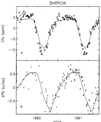
5.2. Point Barrow, Alaska, 71øN (NOAA-CU)
Figure 4a shows the simulated monthly means of CO2 and
8•80 at Barrow
together
with the NOAA-CU measurements.
Both model results and observations are detrended. The 8•80
annual cycle simulated for 1990 is repeated identically two times and plotted against the observations during the interval
2.5 1.5 O5 -O5 -15, -90 ß NOAA-CU ne I• •, ß
SCRIPPS-CIO network s•tes • .. ß
ß CSIRO
network
sites
x...•..
IXl •
ß
- D•
Model
output
ot
eoch
network
s•te
- --...
Totel • IXl ß .... Leoves -"--1•...I xl ' Fossil • Defer -- - Oceon Ixl ß _ • r- ß ß --
NZD KER SMO LIN It!lJOI LJO BRW ALT
-60 -50 0 50 60 c letitude
Figure
3. Zonally
averaged
latitudinal
profile
of 8•80 in CO2 at the surface.
The different
curves
separate
the exchange
with leaves,
soils,
ocean,
fossil
emissions,
and biomass
burning.
Note that the 8•80 profiles
pertaining to each reservoir are not additive but rather combine linearly to yield the resultant 8•80 curve in
solid
line. Solid
symbols
correspond
to the 8•80 simulated
at the precise
location
of the air sampling
sites
and
are the average of atmospheric data measured on flasks samples by NOAA-CU (squares), Scripps-CIO (diamonds), and by CSIRO (triangles). At least 2 years of data have been averaged in the atmospheric
CIAIS ET AL.' STUDY OF A180 IN ATMOSPHERIC CO2, 2 5879 5 BARROW -lO
o
-0.5 199o 1991 YEARFigure 4a. Atmospheric
CO2 and 8180 simulated
at Point
Barrow, Alaska (71øN), compared with the NOAA-CU flask measurements. Both the data and the model output have been detrended.
1990-1991. The model matches well the observed seasonality of the CO2 annual cycle, but it underestimates the peak-to- peak amplitude by about 3 ppm. The simulated 8180 seasonal cycle is in very good agreement with the seasonality of the observations. The model reproduces well the observed position of the minimum in 8180 during October-November. The sim- ulated peak-to-peak amplitude of 8•80 at Barrow is 1.44%o compared to a range of 1.2-1.5%o in the NOAA-CU measure-
ments.
Figure 4b separates 8180 at Barrow into its different com- ponents. The seasonality in 8•80 due to fossil emissions and ocean exchange is negligible. The isotopic exchange with soils contributes roughly 3/4 of the total amplitude and largely de-
termines
the phase
of the simulated
total 8180. Specifically,
Figure 4b indicates that the October-November minimum in
total 8180 at Barrow
is due to soil
exchange,
resulting
from the
seasonal
variation
of 8180 in soil CO2 multiplied
by the • flux
(see part 1, equation (3)). In order to confirm this hypothesis we calculated the average 8180 of soil CO2 over the Siberian region (the region which exerts the largest influence on the concentrations at Barrow) and verified that this variable reaches a minimum in October-November. At this time of the
year the • flux is still large enough for such a minimum in 8180 of soil CO• to have a significant imprint on the atmospheric
8180
at Barrow
(• in fall over
Siberia
is --•30%
of its maximum
level in August).
Figure 4b also suggests that canopy exchange has a smaller influence than soils on the seasonality of 8180 at Barrow, contributing a slight increase in 8180 from April to June and then virtually no change between August and December. Such
BARROW 1 5 - 1 0 - -1 0 Fossil fuels ... Biomass burning -•'Ocean Leaves Soils 0 3 6 9 12 Year
Figure 4b. Modeled
8•80 decomposed
into components
resulting
from exchange
with each
reservoir
sep-
arates. Triangles, leaves; squares, soils; short dashed line, ocean; long dashed line, fossil emissions; solid line, biomass burning.
5880 CIAIS ET AL.: STUDY OF A180 IN ATMOSPHERIC CO2, 2 2.5 -2.5 -5 0.5 -0.5 MAUNA LOA 1988 1989 YEAR
Figure 5a. Atmospheric
CO
2 and/3•80
simulated
at Mauna
Lea, Hawaii (3400 m, 19øN), compared with the Scripps-CIO flask measurements. Both the data and the model output have been detrended.
a weak influence of the leaf isotopic exchange on the season-
ality of total /3•80 at Barrow,
especially
during
the growing
season is surprising. It can be explained by equation (7) of part 1, in which the canopy isotopic disequilibrium flux is treated as
the product
of the retrodiffused
flux of CO2 and/3•80
in leaf
CO2. The simulated monthly mean /3•80 of leaf CO2 over Siberia is nearly constant during the summer and the fall. As
the/3•80 in leaf CO2 is a decreasing
function
of temperature
and an increasing
function
of/3•80 in leaf water (part 1, equa-
tion (12)), higher temperatures in summer compensate for
higher
/3•80 in leaf CO2. In spring,
however,
relatively
cold
temperatures
cause/3•80
to rise in leaf CO2, contributing
the
increase
in May-June
in the vegetation/3•80
exchange
at Bar-
row on Figure 4b.
5.3. Mauna Lea, Hawaii, 19øN (Scripps-CIO)
Figure 5a shows the observed and simulated seasonal cycle
of CO2 and •80 at Mauna
Lea, a station
located
at sigma
level
3 in the TM2 model. Both model results and observations are
detrended.
We have
repeated
two times
the •x80 annual
cycle
simulated for 1990 and plotted it against observations during the 1988-1989 period. Our model underestimates the peak-to- peak amplitude in CO2 by 2 ppm at Mauna Lea, although the
phase
is approximately
correct.
The simulated
•x80 peak-to-
peak amplitude is also too small in our model (0.4%o) com- pared to the Scripps-CIO measurements (0.6%o). On the other
hand,
the phase
of the •x80 model
curve
is realistic
and indi-
cates
that •x80 at Mauna
Lea is maximum
in June-July,
then
decreases sharply during August to reach a minimum in Sep-
tember-October.
The lag of the •mO versus
CO2 minimum
at
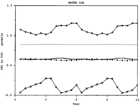
1.5 MAUNA LOA 1.0 0.5 -0.0 ' ' • ' ' i , , • , , 0 3 6 9 12 Year
Figure 5b. Modeled
atmospheric
8180 decomposed
into components
resulting
from exchange
with each
reservoir separates. Triangles, ]caves; squares, soils; short dashed line, ocean; long dashed line, fossil emis- sions; solid line, biomass burning.
CIAIS ET AL.: STUDY OF A180 IN ATMOSPHERIC CO2, 2 5881 2.5 -2.5 0.5 CAPE GRIM
•
. , . •
. , . •
o
• 0 o -0.5 984 1985 1986 1987 1988 1989 1990 1991 YEARFigure 6a. Atmospheric
CO2 and 8180 simulated
at Cape
Grim, Tasmania
(41øS).
The 8180 is from the CSIRO flasks
and CO2 from the NOAA flasks. Both the data and the model
output
have
been
detrended.
The dashed
line in the 8180
plot
is a periodic fit to the data composed of four harmonics.
Mauna Loa is less than a month, compared to 2 months at Barrow.
Figure
5b separates
81sO
at Mauna Loa into its different
components. As is the case at Barrow, the isotopic exchange with soils is found to be the dominant component of the sea- sonal cycle. However, canopy exchange contributes propor-
tionally
more to the seasonality
of total 8180 at Mauna Loa
than at Point Barrow (1/3 for leaves versus 2/3 for soils). Leaf
isotopic
exchange
causes
an increase
in 8180 at Mauna
Loa by
0.2%0 during July-August, then a plateau between August and December followed by a decrease of 0.2%0 in January- February. The ocean and fossil fuel components both induce a
weak
seasonality
in 8180,
which
is due
primarily
to the seasonal
variation in atmospheric transport.
5.4. Cape Grim, Tasmania, 41øS (CSIRO)
Figure
6a compares
the modeled
CO2 and 8180 at Cape
Grim to the measurements made on air samples collected and
analyzed
at CSIRO between
1982
and 1992
for 8180 (the CO2
data are from NOAA flasks). Since our model does not include
any year-to-year
variability
in the 8180 sources,
we have re-
peated the 8180 annual
cycle simulated
for 1990 over the
interval 1984-1992. The detrended observations have been fitted with a periodic function containing four harmonics. The
model
correctly
simulates
the phase
of 8180 at Cape Grim,
with a maximum in December (summer) and minimum in June (winter). The simulated peak-to-peak amplitude (0.35%0) is
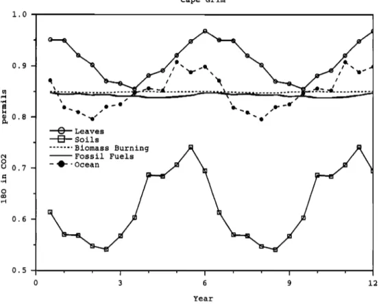
1.0 Cape Grim 0.9 ' ß 0.8 rO 0.7-
'0%,
'0
/
%*0
v Leaves D Soils ... Biomass Burning-
.Fossil Fuels
0.5 ' ' • ' ' t ' ' t ' ' 0 3 6 9 12 YearFigure 6b. Model atmospheric
8180 decomposed
into components
resulting
from exchange
with each
reservoir separates. Triangles, leaves; squares, soils; short dashed line, ocean; long dashed line, fossil emis- sions; solid line, biomass burning.
5882 CIAIS ET AL.: STUDY OF /•180 IN ATMOSPHERIC CO2, 2
1.6 times larger than the average observed peak-to-peak am- plitude during 1982-1992 (0.21%0). Note that we do not apply any selection criteria on the model output to account for the fact that flasks are sampled only when the air comes from a "clean air" sector. According to Ramonet and Mortfray [1996], selecting the model output for the clean air sector at Cape Grim substantially damps the seasonal cycle of CO2 at Cape Grim by removing large synoptic anomalies associated to non- background conditions.
Figure 6b separates 8•80 into its different components. The ocean contributes 40% of the total 8•80 amplitude at Cape Grim, and the biosphere (vegetation plus soils) contributes 60%. Fossil CO2 has a negligible impact on the seasonal cycle of 8•80. The seasonal cycle due to ocean isotopic exchange is minimum in May and maximum in October-December. It is not obviously correlated with the seasonal cycle of SST in the southern ocean since during the Austral summer, warmer SSTs
decrease
the 8•80 of CO2 in seawater
(part 1, equation
(16)).
The exchange with the land biota causes 8•80 at Cape Grim to be higher in summer and a lower in winter. Ramonet [1994] calculates that at 40øS the effects of biospheric exchange in the northern and southern hemispheres are roughly in phase after a lag of about 6 months due to atmospheric transport.
The 8•80 10-year
record
of Cape Grim from Francey
et al.
[1995, Figure 4] indicates that significant year-to-year varia- tions occur whose origin is not clearly known. It is likely that
interannual
variations
in the sources
of •80 may have
caused
the large positive anomalies observed in 1983-1984, 1987- 1988, and 1990-1991. Strong 8180 positive anomalies appear to occur soon after an E1 Nifio event. Considering that E1 Nifio episodes are associated with anomalously high SSTs over the eastern Pacific, it is possible that the ocean cooling associated with a return to normal conditions after an E1 Nifio year may cause a small increase in 8•80. However, the biosphere on land is also likely to have contributed to the interannual variations in the 8•80 of atmospheric CO2, linked to changes in photosyn- thesis, respiration [Keeling et al., 1995] and in global hydrology.
6. Conclusions
We have calculated the atmospheric distribution of the 8•80 in atmospheric CO2 resulting from exchange with leaves, soils, ocean, and anthropogenic emissions. The monthly exchange fluxes derived in part 1 have been run in the 3-D atmospheric
transport
model
TM2 in order
to simulate
the field of 8•80 in
atmospheric CO2 on a 7.5 ø horizontal grid at nine vertical levels. The simulated 8•80 values have been compared to re- cent measurements made by three independent air sampling programs at NOAA-CU, Scripps-CIO, and CSIRO.
As anticipated by the previous study of Farquhar et al. [1993], which did not explicitly include the atmospheric trans- port, we found that the terrestrial biosphere dominates the spatial and seasonal variations of atmospheric 8•80 values, whereas the oceanic exchange plays a relatively minor role. Our main result is that vigorous •80 exchange with soils is primarily responsible for the persistent depletion in 8•80 over the high latitudes of the northern hemisphere. Leaf isotopic exchange opposes this effect by causing an isotopic enrichment in the northern hemisphere. In the tropics we predict a deple-
tion in •80 of CO2 over
regions
covered
by tropical
evergreen
forests, an interesting result that would need to be tested against data from continental sites, for example, by airborne measurements. Overall, the annual ecosystem respiration
strongly modulates the shape of the latitudinal profile in 8•80. Since the annual mean respiration roughly equals the uptake by photosynthesis, we believe that 8•80 does yield independent information on the large-scale geographical distribution of the gross terrestrial carbon fluxes.
We have also examined the seasonality of 8180 at a few sites
and find that the 8180 seasonal
cycle
is controlled
by the
temporal variation in respiration and photosynthesis. In the northern hemisphere a detailed study of the seasonal cycle at Point Barrow and Mauna Loa underscores the key influence of soil respiration in explaining the observed phase lag of 8180 versus CO2. Finally, at Cape Grim in the southern hemisphere, the ocean appears to contribute roughly one third of the ob- served seasonal cycle. The long time series of Cape Grim suggests that large interannual variations are superimposed to the average seasonal cycle.
At this stage the 8180 of CO2 can not yet be used quanti- tatively to infer the terrestrial fluxes of CO2 because we did not examine the sensitivity of our calculations to the prescribed parameters of the model. Of particular importance are the
factors that control 8180 of water in the soil and in chloro-
plasts, mainly the isotopic composition of water vapor and the relative humidity within the canopy. Another important im- provement would be to design a global model of the isotopic composition of CO2 which includes both a coupling of photo- synthesis with climate as already done in SiB2 and a parame- terization of the isotopic composition of water. In addition, the atmospheric transport should be entirely consistent with the calculated surface fluxes.
Acknowledgments. We thank J. M. Hirtzmann and S. Fauquet for
carrying out a preliminary modeling study. We are especially grateful
to G. D. Farquhar, C. A.M. Brenninkmeijer, and K. Rozanski for
helpful discussions on this work. P. Gemery, D. Young, C. Brock, D. Bryant, D. Decker, and S. Webb made the isotopic analysis of the
NOAA/CU flasks. T. Conway and N. Zhang are responsible for the
analyses of CO2, and L. Waterman is responsible for the logistics of the NOAA/CMDL network. We thank the Cape Grim Baseline Air Pol-
lution Station, the Australian Antarctic Division, and the CSIRO's
GASLAB for the Cape Grim and south pole data. Partial support was provided by the Ocean and Atmosphere Carbon Exchange Study and the Atmospheric Chemistry projects of the Climate and Global Change Program of NOAA and by the Atmospheric Research and
Exposure Assessment Laboratory of the EPA. The French Programme
National d'Etude de la Dynamique du Climat and Commissariat h
l'Energie Atomique also contributed to funding. Support is also pro- vided by the EC program ESCOBA.
References
Allison, C. E., R. J. Francey, and H. A. Meijer, Recommendations for
the reporting of stable isotope measurements of carbon and oxygen
in CO 2 gas, in References and Intercomparison Materials for Stable
Isotopes of Light Elements, Proceedings of a Consultants Meeting Held
in Vienna, 1-3 December 1993, IAEA-TECDOC-825, pp. 155-162, Int. At. Energy Agency, Vienna, 1995.
Baertchi, I. H., and W. C. Macklin, Absolute 180 content of standard
mean ocean water, Earth Planet. Sci. Lett., 31,341-344, 1965. Ciais, P., et al., A three-dimensional synthesis study of 8180 in atmo-
spheric CO2, 1, Surface fluxes, J. Geophys. Res., this issue.
Conway, T. J., P. P. Tans, L. S. Waterman, K. W. Thoning, D. R. Kitzis,
K. A. Masarie, and N. Zhang, Evidence for interannual variability of
the carbon cycle from the National Oceanic and Atmospheric Ad-
ministration/Climate Monitoring and Diagnostic Laboratory Global
Air Sampling Network, J. Geophys. Res., 99, 22,831-22,855, 1994.
Denning, A. S., I. Y. Fung, and D. A. Randall, Latitudinal gradient of
atmospheric CO2 due to seasonal exchange with biota, Nature, 376,
CIAIS ET AL.: STUDY OF A180 IN ATMOSPHERIC CO2, 2 5883
Erickson, D. J., III., A stability dependent theory for air-sea exchange,
J. Geophys. Res., 98, 8471-8488, 1993.
Farquhar, G. D., J. Lloyd, J. A. Taylor, L. B. Flanagan, J.P. Syvertsen,
K. T. Hubick, S.C. Wong, and R. Ehleringer, Vegetation effects on
the isotope composition of oxygen in atmospheric CO2, Nature, 363,
439-443, 1993.
Francey, R. J., and P. P. Tans, Latitudinal variation in oxygen-18 of
atmospheric CO2, Nature, 495-497, 1987.
Francey, R. J., F. J. Robbins, C. E. Allison, and N. G. Richards, The
CSIRO global survey of CO2 stable isotopes, in Baseline Atmospheric
Research Program (Australia) 1988, edited by S. R. Wilson and G. P.
Ayers, pp. 20-27, Common. Sci. Ind. Res. Organ. Div. Atmos. Res.,
Melbourne, Victoria, Australia, 1990.
Francey, R. J., C. E. Allison, and E. D. Welch, The l 1-year high
precision in situ CO2 stable isotope record from Cape Grim, 1982-
1992, in Baseline Atmospheric Research Program (1992), edited by C. Dick and P. J. Fraser, pp. 16-25, Commw. Sci. Ind. Res. Organ. Div.
Atmos. Res., Melbourne, Victoria, Australia, 1995.
Friedman, I., and J. R. O'Neill, Compilation of stable isotope fraction-
ation factors of geochemical interest, Pap. 440-KK, U.S. Geol. Surv.,
Reston, Va., 1977.
Gemery, P. A., M. Trolier, and J. W. C. White, Oxygen isotope ex- change between carbon dioxide and water following atmospheric
sampling using glass flasks, J. Geophys. Res., 101, 14,415-14,420,
1996.
Heimann, M., The Global Atmospheric Tracer Model TM2, Dsch. Kli-
marechenzentrum Modellbetreuungsgruppe, Hamburg, Germany,
1995.
Heimann, M., and C. D. Keeling, A three dimensional model of at-
mospheric CO2 transport based on observed winds, 2, Model de-
scription and simulated tracer experiments, in Aspects of Climate
Variability in the Pacific and Western Americas, Geophys. Monogr.
Ser., vol. 55, edited by D. H. Peterson, pp. 237-275, AGU, Wash- ington, D.C., 1989.
International Atomic Energy Agency (IAEA), Statistical treatment of environmental isotope data in precipitation, Tech. Rep. Ser. I.A.E.A.,
206, 1-256, 1981.
Jouzel, J., G. L. Russell, R. J. Suozzo, R. D. Koster, J. W. C. White, and W. S. Broecker, Simulations of the HDO and H 2 •80 atmo-
spheric cycles using the NASA/GISS general circulation model: The
seasonal cycle for present-day conditions, J. Geophys. Res., 92,
14,739-14,760, 1987.
Keeling, C. D., Piper, S.C., and M. Heimann, A three-dimensional
model of atmospheric CO2 transport based on observed winds, 4,
Mean annual gradients and interannual variations, in Aspects of
Climate Variability in the Pacific and Western Americas, Geophys.
Monogr. Ser., vol. 55, edited by D. H. Peterson, pp. 305-363, AGU,
Washington, D.C., 1989.
Keeling, C. D., T. P. Whorf, M. Wahlen, and J. Van der Plicht, Interannual extremes in the rate of rise of atmospheric carbon
dioxide since 1980, Nature, 375, 666-670, 1995.
Louis, J. F., A parametric model of vertical eddy fluxes in the atmo-
sphere, Boundary Layer Meteorol., 17, 187-202, 1979.
Mook, W. G., and J. Jongsma, Measurement of the N20 correction for
13C/12C ratios of atmospheric CO2 by removal of N20, Tellus, 39, 96-99, 1987.
Mook, W. G., M. Koopmans, A. F. Carter, and C. D. Keeling, Sea-
sonal, latitudinal, and secular variations in the abundance and iso-
topic ratios of atmospheric carbon dioxide, 1, Results from land
stations, J. Geophys. Res., 88, 10,915-10,933, 1983.
Ramonet, M., Variabilitd du CO2 atmosphdrique en r•gions australes:
Comparaison modele et mesures, Ph.D. thesis, Univ. Paris XI, Paris,
1994.
Ramonet, M., and P. Monfray, CO2 baseline concept in 3-D atmo- spheric transport models, Tellus, Ser. B, 48, 502-520, 1996.
Tiedke, M., A comprehensive mass flux scheme for cumulus parame-
trization in large-scale models, Mon. Weather Rev., 117, 1779-1800,
1989.
Trolier, M., J. W. C. White, P. P. Tans, K. A. Masarie, and P. A.
Gemery, Monitoring the isotopic composition of atmospheric CO2:
Measurements from the NOAA global air sampling network, J.
Geophys. Res., 101, 25,897-25,916, 1996.
J. A. Berry, Department of Plant Biology, Carnegie Institution of
Washington, 290 Panama Street, Stanford, CA 94305. (e-mail:
P. Ciais, LMCE, CEA l'Orme des Merisiers, Commissariat h
l'Energie Atomique, B•timent 709, Saclay 91191 Gif sur Yvette,
France. (e-mail: [email protected])
G. J. Collatz and P. J. Sellers, NASA Goddard Space Flight Center,
MC 923, Biosphere Sciences Branch, Greenbelt, MD 20771.
A. S. Denning and D. A. Randall, Department of Atmospheric
Sciences, Colorado State University, Fort Collins, CO 80523-1370.
(e-mail: scøtt@abyss'atmøs'cøløstate'edu)
R. J. Francey, Division of Atmospheric Research, CSIRO, PMB Aspendale, Melbourne, Victoria 3195, Australia.
M. Heimann, Max-Planck Institut ffir Meteorologie, Bundestrasse 55, D-20146 Hamburg, Germany.
H. A. J. Meijer, CIO, University of Groningen, 9722 JX Groningen,
Netherlands. (e-mail: [email protected])
P. Monfray, Centre des Faibles Radioactivit•s, Bfitiment 709/
LMCE, 91191 Gif sur Yvette, France.
P. P. Tans, Climate Monitoring and Diagnostic Laboratory, NOAA,
ERL 3, 325 Broadway, Boulder, CO 80303.
M. Trolier and J. W. C. White, Institute of Arctic and Alpine Research, University of Colorado, Campus Box 450, Boulder, CO
80303.
(Received November 18, 1995; revised June 25, 1996; accepted July 12, 1996.)