Regional disparities in mortality by heart attack: evidence from France

HAL Id: halshs-00586837

https://halshs.archives-ouvertes.fr/halshs-00586837

Preprint submitted on 18 Apr 2011

HAL is a multi-disciplinary open access archive for the deposit and dissemination of sci-entific research documents, whether they are pub-lished or not. The documents may come from

L’archive ouverte pluridisciplinaire HAL, est destinée au dépôt et à la diffusion de documents scientifiques de niveau recherche, publiés ou non, émanant des établissements d’enseignement et de

Regional disparities in mortality by heart attack:

evidence from France

Laurent Gobillon, Carine Milcent

To cite this version:

Laurent Gobillon, Carine Milcent. Regional disparities in mortality by heart attack: evidence from France. 2008. �halshs-00586837�

WORKING PAPER N° 2008 - 12

Regional disparities in mortality by heart attack:

Evidence from France

Laurent Gobillon Carine Milcent

JEL Codes: I11, C41

Keywords: spatial health disparities, stratified duration model

P

-

S

E

L

’E

A

-

48,BD JOURDAN –E.N.S.–75014PARIS TÉL. :33(0)143136300 – FAX :33(0)143136310

Regional disparities in mortality by heart attack:

evidence from France

Laurent Gobillon

Carine Milcent

February 21, 2008

Abstract

This paper studies the determinants of the regional disparities in the mortality of patients treated in a hospital for a heart attack in France. These determinants can be some di¤erences in patient characteristics, treatments, hospital charateristics, and local healthcare market structure. We assess their importance with an exhaustive administrative dataset over the 1998-2003 period using a strati…ed duration model. The raw disparities in the propensity to die within 15 days between the extreme regions reaches 80%. It decreases to 47% after controlling for the patient characteristics and their treatments. In fact, a variance analysis shows that innovative treatments play an important role. Remaining regional disparities are signi…cantly related to the local healthcare market structure. The more patients are locally concentrated in a few large hospitals rather than many small ones, the lower the mortality. Keywords: spatial health disparities, strati…ed duration model

JEL code: I11, C41

We are grateful to Marteen Lindeboom, Thierry Magnac, Francesco Moscone and Jordan Rappoport for very

useful discussions, as well as the participants of the 16th EU Health Econometrics Workshop in Bergen and the

54th NARSC in Savannah. This project was carried out with the …nancial support of the French Direction of Research, Studies, Evaluation and Statistics (DREES). We are responsible for all remaining errors.

y_{INED, 133 boulevard Davout, 75980 Paris Cedex. Tel: 0033(1)56062016. Email: laurent.gobillon@ined.fr.}

Webpage: http://laurent.gobillon.free.fr.

z_{PSE (CNRS-EHESS-ENPC-ENS), 48 boulevard Jourdan, 75014 Paris. email: milcent@pse.ens.fr. Webpage:}

1

Introduction

Spatial disparities in heath outcomes have become a major concern in France. A driver of these disparities is often thought to be the missallocation of ressources caused by a lack of information on local needs. As a consequence, a reform in 1996 decentralized the funding of the healthcare system at the regional level. A global budget is now decided nationally before being dispatched between regions. Some public regional agencies allocate the regional budgets between local public and private not-for-pro…t hospitals after some bargaining.

Importantly, it is not obvious whether changing the regional budgets is likely to have a sizable e¤ect on regional disparities in outcomes. The e¤ect will be signi…cant if supply factors (like hospital capacities or equipments) are distributed unevenly over the territory and these factors a¤ect health outcomes signi…cantly. By contast, changing regional budgets will have a far smaller e¤ect if health outcomes are mainly the result of demand factors (like the age structure and socio-economic habits). Also, the way regional agencies should allocate their regional budget between hospitals is debatable. It is not clear-cut whether it is more e¢ cient to have a few well-equipped hospitals which concentrate all the patients or many small hospitals which cover well the whole regional territory.

In this paper, we quantify the spatial disparities in the mortality of patients treated in a hospital for an acute myocardial infarction (heart attack). We then assess the importance of demand and supply factors in explaining these disparities.

In the economic literature on health outcomes, most of the papers focus on the e¤ect of supply factors, using demand factors only as controls. In that perspective, regional disparities in out-comes may depend on the local management of patients after their admission in hospitals. This management is related both to the quick admittance of patients in an adequate hospital and the quality of care that they receive. A large literature focuses on the e¤ect of ownership on hospital performance. Many authors compares for-pro…t and not-for-pro…t institutions (McClellan and staiger, 2000; Hansman, 1996; Milcent, 2005). Some others study the change in ownership status (Propper, Burgess and Green, 2004).1 _{However, these papers do not assess whether there is some}

sorting of hospitals depending on their ownership status that could lead to spatial disparities in performances. Also, they do not look much on the e¤ect of treatment quality provided by hospitals on outcomes whereas there is an extensive literature in epidemiology on this issue for heart attack

1_{Other papers related to the topic include Newhouse, 1970; Cutler and Horwitz, 1998; Silverman and Skinner,}

(see for instance Jollis et al., 1994). Some spatial disparties in the quality of treatments, possibly related to the local proportions of hospitals in each ownership status, may cause some spatial disparities in outcomes. We will address this kind of issues in our study.

In fact, the international literature on spatial health disparities is still scarce. There are some comparisons between countries in the horizontal equity in health care utilization (see van Doorslaer et al., 1997, 1999, 2000). However, for studies on a given country, space is usually not the main topic and it is rather used as an extra-dimension to construct some instruments. For instance, Geweke, Gowrisankaran and Town (2003) explain the hospital choice with the distance between the place of residence and hospitals. There are a few exceptions like Mobley (2003) who studies the e¤ect of the local healthcare structure on prices, but the emphasis is on healthcare acces rather than on health outcome. Milcent (2005) evaluates the e¤ect of space on the mortality of patients admitted in a hospital for a heart attack but only through the distance between the place of residence and the hospital which is found to have a non-signi…cant e¤ect. In fact, it is quite possible that the local healthcare market structure has an e¤ect on the local hospital performances. We may think that local interactions and competition, as well as the local concentration of patients in a few hospitals to bene…t from economies of scales, may a¤ect the local outcomes. These issues deserve more attention.

By contrast, the literature on spatial disparities in the …elds of economic geography and urban economics has developed a lot in recent years. Some papers try to assess to what extent spatial disparities in wages (Duranton and Monastiriotis, 2004; Combes, Duranton and Gobillon, 2008) or unemployment (Gobillon, Magnac and Selod, 2007) can be explained with workers’composition e¤ects, …rm e¤ects and true location e¤ects. We will borrow some tools from this literature as the setting is quite similar.

For our study, we construct a unique matched patients-hospitals dataset from some exhaustive French administrative records over the 1998-2003 period. This original dataset contains some information on the demographic characteristics of patients, their diagnoses and their treatments. It also provides some details on the hospitals where the patients are treated like the location, the ownership status and the capacity. We show that regional disparities in mortality are quite large. In particular, the raw di¤erence in the propensity to die within 15 days between the extreme regions reaches 80%. We then assess whether these spatial disparities come from some local di¤erences in patient characteristics (demographic shifters and secondary diagnoses), treatments, hospital characteristics or healthcare market structure. We …rst estimate at the patient level a

Cox duration model strati…ed by hospital (i.e. each hospital has a speci…c baseline hazard) using the Strati…ed Partial Likelihood Estimator proposed by Ridder and Tunali (1999). This estimator allows to recover the e¤ect of the patient-speci…c variables (their characteristics and treatments) while controlling for hospital unobserved heterogeneity. We then reconstruct the survival functions of hospitals net of individual e¤ects and average them at the regional level. We …nd that remaining regional disparities are lower but are still signi…cant. The di¤erence in the propensity to die within 15days between the extreme regions is now 47%. A variance analysis at the regional level shows that regional di¤erences in innovative treatments play an important role.

We then assess to what extent the remaining regional disparities can be explained with some hospital and geographic characteristics. For that purpose, we …rst specify the hospital hazards as the product of some hospital …xed e¤ects and a baseline hazard. We show how to recover the hospital …xed e¤ects using some moment conditions. We then regress the hospital …xed e¤ects on some hospital and regional variables. Finally, we average the model at the regional level and conduct a variance analysis. We …nd that the local concentration of hospital supply plays a signi…cant role. The more patients are concentrated in a few large hospitals rather than many small ones, the lower the mortality. After hospital and geographic variables have been controlled for, some unexplained regional disparities still remain.

In a …rst section, we present how the French healthcare system deals with patients admitted in a hospital for an acute myocardial infarction. A second section describes our dataset. We then present in a third section some descriptive statistics on the regional disparities in mortality, demand factors and supply factors. The fourth section details the econometric methodology used to identify the causes of the regional disparities in mortality. The …fth section summarizes the results of the model.

2

Heart attack in the French context

2.1

Healthcare organization

In France, there are two types of ownership: public and private. For public hospitals, all in-frastructures, equipments and sta¤ belong to the public sector. Investment in public hospitals are …nanced by public funding. The sta¤ (including doctors and nurses) consists in salaried civil servants. For private hospitals, infrastructures, equipments and sta¤ belong to the private sec-tor. The non-doctor sta¤ is salaried. Part of the doctor sta¤ is salaried and the other part is

self-employed.

The public sector is under a global budget system. Part of the private sector is under the same global budget system. Private hospitals which bene…t from this budget are called not-for-pro…t hospitals (NFP). Every year, the government determines the global budget and chooses how to divide it between regions (see Graph A1 for a map of the French regions). The regional budget is dispatched between NFP and public hospitals through bilateral bargaining between the regional regulator and the directors of hospitals. Since the Juppé reform in 1996, the bargaining power of regional regulators has increased signi…cantly and regional local authorities have gained more in‡uence on the regional hospital organization. NFP and public hospitals should grant access to hospital care to every patients. They cannot make any pro…t. Hospitals in the private sector (excluding NFP) are paid by fee-for-services and can select patients. The selection is usually done to maximize pro…t taking into account the socio-economic caracteristics of patients (like solvability) and their health. These hospitals have no constraint on pro…ts and are called for-pro…t hospitals (FP).

All these di¤erences suggest that hospitals have di¤erent incentives to provide health care to patients depending on their status (public or private) and mode of reimbursment (fee-for-service or global budget). This is particularly true for innovative procedures that are costly. Indeed, for-pro…t hospitals are …nanced via a fee-for-service system. Supplies such as stents are reimbursed ex-post in addition to the fee-for-service payment. Doctors have an incentive to perform innovative procedures as they receive additional fees for performing them. By contrast, it is more di¢ cult for public and not-for-pro…t hospitals to purchase expensive devices as the public budget does not account for costly innovative procedures (catheterization, angioplasty or stent). However, these hospitals still perform some innovative acts (Dormont and Milcent, 2006). In fact, doctors may have some indirect incentives to perform innovative procedures such as improving their reputation or learning by doing.

Individuals do not have the same access to health care depending on the hospital status and the mode of reimbursment. Patients are not charged in public hospitals except for a small out-of-pocket but they incur charges in private hospitals. By contrast, for-pro…t hospitals …x the price of cattering and procedures, and patients are reimbursed on the basis of public hospital charges only. The di¤erence between the price and reimbursment can be huge. The situation is intermediate in not-for-pro…t hopitals as they only …x the price of cattering.

2.2

Treatments of heart attack

In this paper, we focus on one single disease. Indeed, evidence shows that the e¤ect of character-istics (sex, age, ...) on mortality is disease-speci…c (Wray et al., 1997). We selected the Acute Myocardial Infarction (heart attack) for four reasons. First, it belongs to the ischemic-disease group that has been the primary cause of mortality in France, before getting second recently after cancer. Second, mortality from AMI has been widely studied in the literature to assess the quality of hospital care in the US and the UK. This literature can by used for comparison (see Goworisakaran and Town, 2002, for the US, and Propper, Burgess and Green, 2004, for the UK). Third, AMI is a well-de…ned pathology with only a few re-admission due to its clinical de…nition. Fourth, mortality from AMI is an event frequent enough to yield some reliable statistical results. We focus only on the stays of patients who arrived at the hospital after a heart-attack crisis. This sample includes people who were told by their doctor to go to the hospital because of a heart problem and those who were transferred from an emergency unit to a cardiac care unit. We leave aside stays in emergency units when patients died or where sent back home. Indeed, the health of patients in emergency units is usually not stabilized and these patients cannot be cured with the usual treatments which are risky and can cause brutal death.

Before patients arrive at the hospital or when they just get in, they may receive thrombolytic drugs. In the hospital, patients can bene…t from various treatments and procedures. These include cardiac catheters (denoted as CATH hereafter), percutaneous transluminal coronary angioplasty (PTCA), stent and bypass surgery. A catheter is a ‡exible and thin pipe which is installed in a vein to facilitate injections and drips. It may also be used to clean arteries to improve the blood ‡ow. A bypass surgery reroute, or “bypass”, is a vein or artery collected on the patient’s body and set up to derive blood from coronary arteries to avoid clogged sections. It allows to improve the blood ‡ow and the oxygenation of the heart. The angioplasty and the stent are some alternatives to the bypass to improve the blood ‡ow in clogged arteries. They are used when arteries are too clogged. An angioplasty consists in in‡ating a balloon in a blockage to create a channel. This procedure is costly as it induces for one stay an increase in costs which ranges from 30% to 60% (Dormont and Milcent, 2002). The stent is a spring-shaped prosthesis which is used as a complement to angioplasty. It is put inside the balloon to keep the artery dilated. The use of one or several stents with an angioplasty signi…cantly improves the results. We are going to study the e¤ect of treatments over the 1998-2003 period. Angioplasties and stents were some innovative treatments around 1998 and have generalized such that they are used at wide scale in 2003. In

particular, the use of angioplasty with stent has increased from 15% in 1998 to 31% in 2003. In this article, the term stent will refer to an angioplasty together with one or more stents, the term angioplasty will refer to an angioplasty without stent, and the term catheterism will refer to a catheterism without angioplasty and stent.

2.3

Spatial features

We now propose a spatial overview of heart attack. First note that patients who experience an AMI and want to be treated in a NFP or a public hospital usually have to go to a hospital within their region of residence. However, some patients are sometimes transferred to a neighbouring hospital in another region. Also, a patient who gets sick in another region may be cured there. Over the 1998-2003 period, the proportion of AMI patients treated within their region of residence is very high at 92:9%. This proportion is slightly lower for for-pro…t hospitals (91:4%) than for public hospitals (93:1%) and NFP (95:8%). Together with the regional organization of healthcare, these statictics support the fact that regions can be viewed as local healthcare markets for heart attack.

Depending on their residential location, patients do not face the same supply of healthcare as the local composition of hospitals by status and mode of reimbursment varies widely across space. In 1999, the proportion of beds in public hospitals is large in Franche-Comté (in the east) where it reaches 80% and in the west. By contrast, it is only 46% in the PACA region (in the southern French Riviera). The proportion of NFP is the highest in some eastern regions at the German border (Alsace and Lorraine) for historical reasons. Conversely, the proportion of beds in for-pro…t hospitals is larger in the French Riviera where the population is older and richer.

The local ownership composition of bed capacities is closely related to the local ownership com-position of hospitals where AMI patients are treated. Graph 1 shows that around Paris and in southern regions, the proportion of patients treated in a for-pro…t hospital is higher. These regions often provide more innovative treatments than the others, like stents as shown in Graph 2. In fact, the rank correlation between the proportions of stents and AMI patients in for-pro…t hospitals is :61. When considering NFP hospitals instead of for-pro…t hospitals, the correlation is still quite high at :44.

We also contructed the probability to die within 15 days (see Graph 3).2 _{This probability is}

quite low in the Paris region, the east and south-east. It is larger in the west and south-west. There is no obvious relationship between the probability to die and the proportions of stents or for-pro…t hospitals (rank correlations: :09 and :14 respectively). However, south eastern regions which have a large proportion of for-pro…t hospitals performing innovative treatments also concentrate older people who are more likely to die. Hence, it is necessary to perform an econometric analysis to disentangle the e¤ect of age and more generally from individual attributes (demographic characteristics and secondary diagnosis) from that of hospital composition and treatments.

[Insert Graph 3]

3

The dataset

3.1

Data sources on patients, hospitals and areas

For our study, the primary dataset is the PMSI (Programme de Médicalisation des Systèmes d’Information). This dataset provides the records of all patients discharged from any French acute-care hospital over the 1998-2003 period. It is compulsory for hospitals to provide these records on a yearly basis.3 _{Three nice features of this dataset are that it provides some information}

at the patient level, it keeps track of hospitals across time, and it is exhaustive both for the public and private sectors.4 A limit of the data is that patients cannot be followed across time if they come back again later in the same hospital or if they change hospital.

The dataset contains some basic information on demographic characteristics of patients (age and sex), as well as some very detailed information on diagnoses and treatments. In our analysis, we can thus take into account all secondary coronary diagnoses as well as all technics used to cure patients. The dataset also provides us with the type of entry (whether the patients come from their residence, another care service in the same hospital or another hospital) as well as the type of exit (death, home return, transfer to another hospital or transfer to another care service).

2_{See below for more details on how this probability was computed.}

3_{An exception is local hospitals for which it is not compulsory. This does not a¤ect our study since these}

hospitals do not take care of AMI patients.

We only keep patients whose pathology was coded as an acute myocardial infarction in the tenth international code of disease (ICD-10-CM), i.e. the patients for which the code was I21 or I22. Before 35, heart attacks are often related to a heart disfunction. As a consequence, we restrain our attention to the patients more than 35 following thus the OMS de…nition. After deleting observations with missing values for the variables used in our study (which are only a very few), we end up with 421; 185 stays (in 1; 130 hospitals) over the 1998-2003 period.

We match our dataset with the hospital records from the SAE survey (Statistiques Annuelles des Etablissements de santé) that was conducted every year over the 1998-2003 period. The SAE survey contains some information on the municipality where each hospital is located, the number of beds (in surgery and in total) and the number of days that beds are occupied (in surgery and in total). The matching rate is very good and reaches 97% of the stays (which corresponds to 408; 592stays in 1; 084 hospitals).

The municipality code in the SAE survey also allowed us to match our dataset with some variables at the municipality level coming from other sources. These variables will be used in our estima-tions as proxies to control for the municipality averages of individual unobserved socio-economic characteristics. Indeed, the literature has shown that there can be some large socio-economic disparities in health outcomes (see for instance Lindeboom and van Doorslear, 2004; Etilé and Milcent, 2006). Our municipality variables include the municipal unemployment rate computed from the 1999 population census, the median household income from the 2000 Income Tax dataset and the existence of a poor area in the municipality (poor areas being de…ned by a 1997 law). These indicators should (at least partially) capture some spatial di¤erences in lifestyle that can have an impact on the health of patients and their propensity to die from AMI. Also, thanks to the municipality code, we could identify the urban area in which hospitals are located.5 We computed the local numbers of beds as a measure of the interactions between hospitals within a given urban area. This variable also captures congestion e¤ects and we will be able to estimate only the e¤ect of interactions net of congestion. We also computed a regional Her…ndahl index at the urban area level using the number of patients in hospitals within each urban area. The Her…ndahl index measures for a given urban area to what extent patients are equi-distributed between hospitals or

5_{An urban area is de…ned as an urban center (with more than 5,000 jobs) and the municipalities in its}

catch-ment area. There are 359 urban areas in mainland France and they do not cover the whole territory (as some municipalities are excluded and remain rural).

concentrated within a few hospitals.6 _{When constructing urban area variables, we were confronted}

with a few hospitals in municipalities which do not belong to any areas or to several of them. We thus introduced some dummies for these two cases as controls. As we will use hospital variables which should be time-invariant in our analysis (see Section 4 and 5), all hospital and geographic variables are averaged across years. There are 406; 197 stays (in 1; 080 hospitals) for which we have all the information on hospital and geographic variables.

We do not have any information on what happpened to transferred patients before their transfer. In particular, we do not know how they were treated and how long they have already stayed in a hospital. As a consequence, we restrict our attention to patients who come from their place of residence. We end up with 341; 861 stays (in 1; 105 hospitals) for which all the information is available on patient variables (and 331; 246 stays in 1; 060 hospitals for which all the information is available on hospital and geographic variables).

3.2

Preliminary statistics

For each hospital, we then computed a gross survival function for exit to death using the Kaplan-Meier estimator. This estimator treats other exits (home return and transfers) as censored. As we are mostly interested in hospital disparities across regions, we computed the average survival function by region.7 _{Observations were weighted by the number of patients still at risk in the}

hospitals.8 _{We selected the region with the highest survival function (Alsace), the region with the}

6_{The Her…ndahl index for an urban area u is H}

u= X j2u pj pu 2

where j indices the hospitals, pj is the number of

patients in hospital j, and pu =X

j2u

pj is the total number of patients within the urban area u. Hu increases from

1

Nu to 1 as the concentration of patients increases, where Nu is the number of hospitals in the urban area u. Wen

Hu = _N1_u, the patients are equi-distributed between the Nu hospitals. When Hu = 1, they are all treated within

one hospital.

7_{We could have directly computed a survival function for each region. However, we believe that the relevant}

unit at which the treatment of patients takes place is the hospital. Also, our approach at the hospital level parallels the results obtained for the model presented in Section 5.

8_{When the length of stay increases, the number of patients in a given hospital decreases. Above a given length}

of stay after which there is no patient at risk anymore, it is not possible to estimate the survival function. We then arbitrary considered that the hospital survival functions remained constant after this length of stay. When we compute the average survival functions by region, this assumption does not have much e¤ect for short/medium length of stays. Indeed, only small hospitals do not have any patients at risk anymore for these lengths of stays. As a consequence, we computed our descriptive statistics only for stays below …fteen days to minimize the e¤ect

lowest survival function (Languedoc-Roussillon), and the Ile-de-France region that corresponds mostly to the Greater Paris Area and is the most densely populated. Graph 4 represents the survival functions of these three regions as well as their con…dence intervals (Graph A2 in appendix represents the survival functions for all the regions and Table A1 ranks the regions according to their probability to die within 15 days). It shows that the average survival functions of any two regions are signi…cantly di¤erent.

[Insert Graph 4]

Table 1 reports some disparity indices between regions in the probability to die within 1, 5, 10 and 15 days (de…ned as one minus the Kaplan-Meier). These indices are the max/min ratio, the Gini index and the coe¢ cient of variation. The Gini indices and the coe¢ cients of variation are computed in two stages. First, we compute the average of a given individual variable (for instance, a death dummy) by region. Then, we compute the regional disparity indices for the resulting variable (in our example, the share of deaths in the region), weighting the observations by the number of patients in the region. The max/min ratio shows that regional disparities are signi…cant. Indeed, the di¤erence in the probability to die within 15 days between the Maximum (Languedoc-Roussillon) and the Minimum (Alsace) is 80%. However, more global indices like the Gini index (0:07) and the coe¢ cient of variation (:218) remain quite small and suggest that disparities are not systematic. Interestingly, disparities are a bit larger for the probability of death within 1 day (Max/Min ratio of 94%). This may be due to di¤erent behaviours across regions in transfers and home returns at early days of AMI.

The regional disparities may be explained with some spatial disparities in demand factors (demographic shifters and secondary diagnosis) or in supply factors (treatments, characteristics of hospitals and local healthcare market structure). The purpose of the paper is to disentangle these two types of e¤ects. Potential candidates are built from patient and hospital variables aggregated at the regional level. We now present some regional disparity indices for these candidates. We mostly comment the results obtained for the Gini indices as they are global measures of disparities and they are not sensitive to the level of magnitude as the max/min ratio (alternatively, we could also comment the results obtained with the coe¢ cients of variation which are similar). In the sequel, we will say to ease the presentation that disparities are small when the index is inferior to :1, they are moderate for an index from :1 to :2, they are large for an index from :2 to :3, and they are very large for an index above :3.

We …rst consider variables related to patients which were averaged at the regional level. We …nd that there are signi…cant disparities across regions for some demographic variables: more speci…cally the Gini index is moderate for females aged 35 55 (:12) and males who are more than 85 (:11). For diagnoses, disparities are often moderate or large, the Gini index reaching :23 for surgical French DRGs (.23), :15 for the severity index and :13 for a history of vascular diseases and for stroke. Note that the Gini index is most often moderate for diagnoses related to speci…c behaviours before the heart attack such as obesity (:17), excessive smoking (:16), and alcohol problems (:14). It is smaller for diabetes (:08). For treatments, disparities are often large or very large. The Gini index reaches goes up to :53 for dilatations other than PTCA and :37 for the cabbage or coronary bypass surgery. These two high disparity indices are not surprising as the related treatments are (very) seldomly applied. More usual treatments like angioplasty and stent still have a large Gini index which takes the value :28 and :21, respectively. Disparities are far smaller for the catheter which is a more widespread treatment (:10).

Overall, the Gini indices show that potential explanations of disparities in the propensity to die can be related to the three types of variables: demographic characteristics, diagnoses and treatments. Our econometric analysis will determine which type of explanation has the largest explanatory power.

[Insert T able 1]

We then computed regional disparity indices for the hospital and geographic variables used in our regressions. Whereas hospital variables measure capacities and status (public, for-pro…t and NFP), geographic variables are meant to capture scale economies and local interactions. For a given variable, we constructed its regional average, weighting the observations by the number of patients in the hospitals. The resulting regional average is then used to compute disparity indices at the regional level. Results are reported in Table 2.

As previously, we only comment Gini indices. We begin with hospital variables. There are large disparities across regions in the average size of hospitals measured by the total number of patients (:23) or the number of AMI patients (0:27). Disparities are even larger for the number of beds (:49) and the number of beds in surgery (:47). There disparities point out at some sorting of hospitals according to their size. Finally, disparities are smaller but still large for the hospital status and more speci…cally for being a for-pro…t hospitals (:24).

We now comment the results for geographic variables. We observe some very large disparities in the number of beds in in the urban area (Gini index :66). Disparties are also signi…cant for

the Her…ndhal index computed at the urban area level (:20). Finally, regional disparities in municipality variables used as proxies for unobserved demand factors are at best moderate, the Gini index reaching :17 for the presence of a poor area in the municipality.

[Insert T able 2]

Overall, demand and supply factors both constitute potential candidate to explain the regional disparities in mortality. We now present our empirical methodology to disentangle their e¤ects.

4

Econometric method

We …rst give a brief description of the econometric model before turning to a more formal pre-sentation of our approach. Even if we are interested in studying di¤erences in mortality across regions, we build our model around hospital units. Indeed, hospitals have some speci…c behaviour and e¢ ciency which should be properly accounted for to avoid misspeci…cation biases. Hence, we use a Cox duration model at the patient level strati…ed by hospital. This model contains some patient-speci…c explanatory variables (demographic shifters, diagnoses and treatments), as well as a speci…c survival function for each hospital which is left unspeci…ed. Ridder and Tunali (1999) explain how to estimate this model using the strati…ed partial likelihood estimator (SPLE) and establish the theoretical properties of the estimators. Lindeboom and Kerkhofs (2000) apply their methodology to quantify the e¤ect of school on job sickness of teachers and Gobillon, Magnac and Selod (2007) use it to analyze the e¤ect of location on …nding a job in the Paris region. This methodology is more general than the ones usually used in the health literature on mortality which take into account the hospital unobserved heterogeneity at best with hospital …xed e¤ects (Milcent, 2005). It can be applied even when the sample size and the number of hospitals are large as in our case, whereas it is not even computationally possible to estimate directly some hospital …xed e¤ects. After estimating the hospital survival functions, we average them at the regional level to study the regional disparities in mortality net of the e¤ect of patient-speci…c variables. We then link the remaining regional disparities to some local di¤erences in hospital and geographic characteristics. For that purpose, we make the additional assumption that the hospital hazards write multiplicatively as the product of a hospital …xed e¤ect and a baseline hazard. We show how to estimate the hospital …xed e¤ects using empirical moment conditions. We then explain these …xed e¤ects with hospital and geographic variables and …nally average the model at the regional

level to perform a regional variance analysis.9

We now present our approach more formally. For each patient, we observe the length of stay in the hospital and the type of exit (death, home return or transfer). In the sequel, we only study exit to death. All other exits are treated as censored. We specify the hasard function of a patient i in a hospital j (i) as:

(t_jXi; j (i) ) = j(i)(t) exp (Xi ) (1)

where j( )is the instantaneous hazard function for hospital j, Xiare the patient-speci…c

explana-tory variables and are their e¤ect on death. Insofar, the hospital hazards are left completely unspeci…ed and allow for a very general study of regional disparities in death using regional av-erages. Also, this semi-parametric approach avoids biases on the estimator of coe¢ cients which could arise from a misspeci…cation of the hospital hazards. The model is estimated by strati…ed partial maximum likelihood. The contribution to likelihood of a patient i who dies after a duration ti is his probability to die conditionally on someone at risk in his hospital dying after this duration.

It writes: Pi = exp (Xi ) X i2 j(i)(ti) exp (Xi ) (2)

where j(ti) is the set of patients at risk at day ti in hospital j, i.e. the set of patients that are

still in hospital j after staying there for ti days. The partial likelihood to be maximized then

writes: L =

iPi. Denote b, the estimated coe¢ cients of patient-speci…c explanatory variables. It

is possible to compute the integrated hazard function j(t) of any hospital j using the Breslow

(1974)’s estimator. It writes: b_j(t) = t Z 0 I (Nj(s) > 0) X i2 j(s) exp Xib dNj(s) (3)

where I ( ) is the indicator function, Nj(s) = card j(s), and dNj(s) is the number of patients

exiting from hospital j between the days s and s + 1. From the Breslow’s estimator, we compute a survival function for each hospital j as exp( bj(t))(an estimator of its standard error is recovered

9_{A tempting alternative approach is to estimate all the coe¢ cients in one stage only introducing all the patient,}

hospital and geographic variables in a simple Cox model. However, such an approach does not take into account the hospital unobserved heterogeneity. Consequently, standard errors of the coe¢ cients may be highly biased (see Moulton, 1990). Our approach properly accounts for this issue.

using the delta method). The hospital survival functions will be averaged at the regional level to study regional disparities in mortality after any number of days.

We then study the determinants of hospital disparities by specifying the hospital hazard rates in a multiplicative way:

j(t) = j (t) (4)

where j is a hospital …xed e¤ect and (t)is a baseline hazard common to all hospitals. We show

in appendix how to estimate the parameters using empirical moments derived from (4).10 _Note

that we need an identifying restriction since j and (t) can be identi…ed separately only up to a

multiplicative constant. We impose for convenience that: _N1P

t

Nt (t) = 1where Nt is the number

of patients still at risk at the beginning of day t and N = P

t

Nt. After some calculations (see

appendix), we get: (t) = 1 N2 X j;t NjNt j(t) ! 1 1 N X j Nj j(t) ! (5) j = 1 Nj X t Njt (t) ! 1 1 Nj X t Njt j(t) ! (6) where Njt is the number of patients at risk at time t in hospital j, Nj =

P

t

Njt, and the sum on t,

P

t

, goes from t = 1 to t = T (here, we …x T = 30 for convenience). It is possible to obtain some estimators of (t) and j replacing j(t)by the estimator bj(t) = bj(t) bj(t 1)in the

right-hand side of equations (5) and (6). These estimators are denoted b (t) and_bj. We show in appendix

10_{In doing so, we depart from the log-linear estimation method proposed by Gobillon, Magnac and Selod}

(2007). Our approach is more adequate when exits are scarce as in our case. Indeed, Gobillon, Magnac and

Selod split the timeline into K intervals denoted [tk 1; tk]. Introduce k =

tk

Z

tk 1

(t) dt= (tk tk 1) and yjk =

[ j(tk) j(tk 1)] = (tk tk 1). Integrating (4) over each interval and taking the log, they get: ln yjk = ln j+

ln k. yjkis not observed but can be replaced with a consistent estimator: ybjk =

h

b_j(tk) bj(tk 1)

i

= (tk tk 1).

The equation to estimate is then: lny_bjk= ln j+ ln k+ jkwhere jk= lnbyjk ln yjkis the sampling error. This

equation can be estimated with standard linear panel methods. The authors use weighted least square where the

weights are the number of individuals at risk at the beginning of the interval. A limit of this method is that ln yjk

can be replaced by its estimator lny_bjk only if ybjk 6= 0. When it is not the case, observations should be dropped

from the sample. When implementing this approach to our case, this could be an issue as exits are scarce and a signi…cant number of observations should be dropped when the time spent in the hospitals gets large. In practice however, the results obtained with the two approaches are quite similar.

how to compute the covariance matrices of b = b (1) ; :::; b (T ) 0 and b = (b1; :::;bJ)0. We then

try to explain the hospital …xed e¤ects with some hospital and geographic variables denoted Zj.

We specify: j = exp Zj + j where are the coe¢ cients of hospital and geographic variables,

and _j includes some unobserved hospital and geographic e¤ects. For a given hospital j, taking the log and replacing the hospital …xed e¤ect with its estimator, we get:

ln_bj = Zj + j+ j (7)

where _j = ln_bj ln j is the sampling error on the hospital …xed e¤ect. Equation (7) can be

estimated using weighted least squares where the weight is the number of patients in the hospitals. Gobillon, Magnac and Selod (2007) explain how to compute the standard errors and propose a R-square formula which accounts for the sampling error. We use their formulas in our empirical application. Note that for a given hospital, equation (7) is well de…ned only when there is at least one patient dying in the hospital over the 1998 2003 period (otherwise the quantity _bj from

which we take the log would be zero). This condition may not be veri…ed for hospitals that have only a few patients. In fact, these hospitals have a negligible weight and they are dropped from our sample. We …nally average equation (7) at the regional level and conduct a variance analysis for the resulting equation.

5

Results

Table 3 reports the estimation results of the …rst-stage equation (1). The demographic character-istics have the usual e¤ect on the propensity to die. Females are more likely to die than males. This is consistent with care being more protective for males than for females possibly because of biological di¤erences like the smaller target vessel size and the increased vessel tortuosity of females (Milcent et al., 2007). However, the gender di¤erence is signi…cant only at younger ages (between 35 and 55 year old). Also, the propensity to die increases with age.

The severity index is found to have a positive e¤ect on the propensity to die. Intuitively, one also expects secondary diagnoses to have a positive e¤ect as they deteriorate health. This is true empirically for renal failure, stroke, heart failure, conduction disease, alcohol. Other secondary diagnosis have a more surprising negative e¤ect: diabetes, obesity, excessive smoking, vascular disease, peripheral arterial disease, previous coronary artery disease, hypertension. These results may be explained by preventive health care. Indeed, these secondary diagnoses may point out at

patients who have been monitored more carefully before and after having a heart attack (Milcent, 2005).

All treatments have the expected negative e¤ect on the propensity to die: CABG, catheterism, PTCA, other dilatation and stent. The stent, which is the most innovative procedure, has the strongest negative e¤ect. After controlling for these treatments, the DRG index capturing the heaviness of surgical procedures has a positive e¤et on the propensity to die. This can re‡ect the increased chances to die because of more cumbersome and risky surgery.

[Insert T able 3]

From the estimated coe¢ cients b, we constructed an integrated hazard for each hospital using the Breslow’s estimator and averaged the corresponding hospital survival functions by region (weighting by the number of patients at risk in the hospitals).11 _{Regions at extremes are the}

same as when studying the raw data: Alsace (at the German border) usually exhibits the highest survival function and Languedoc-Roussillon (in the South-East) the lowest. Graph 5 represents the survival functions (as well as their con…dence intervals) for these two extremes and for Ile-de-France (the Paris region).12 The di¤erence between the extreme regions are smaller but still signi…cant.

[Insert Graph 5]

We quantify the regional disparities with the same indices as in the descriptive section 3.2 for the probability to die within 1, 5, 10 and 15 days (de…ned as one minus the survival function of the model). Results reported in Table 4 show that the di¤erence in the probability to die within 15days between the extreme regions has decreased from 80% to 47% (this corresponds to a 41%

11_{This kind of aggregation is quite common in the labour literature. For instance, Abowd, Kramarz and Margolis}

(1999) estimate a wage equation that includes some …rm …xed e¤ects. They then compute some industry …xed e¤ects as the averages of the estimated …rm …xed e¤ects for …rms belonging to each industry (weighting the observations by the number of workers in the …rms).

12_{Graph A3 in appendix represents the survival functions for all the regions and Table A2 ranks the regions}

according to survival after 15 days. Curves obtained with the model are not strictly comparable with those obtained from raw data with the Kaplan-Meier estimator as instantaneous hospital hazards were normalized with an ad-hoc rule. To get close to comparability, we multiplied instantaneous hospital hazards by a constant which was

chosen such that in absence of hospital heterogeneity (i.e. j(t) = (t) for all t), the expected integrated hazard at

day 1 is equal to the expected integrated hazard obtained from the raw data (de…ned as minus the logarithm of the Kaplan-Meier estimator). This normalization allows to obtain an average survival function of the same magnitude as the one obtained from raw data with the Kaplan-Meier estimator.

decrease). More systematic disparity indices like the coe¢ cient of variation and the Gini index also decrease, but to a lesser extent (by 19% and 17%, respectively). In a variance-analysis spirit, we de…ned a pseudo-R2 _{as one minus the ratio between the variance in the probability to die}

within a given number of days computed from the model and the variance computed from raw data. At 1 and 5 days, the pseudo-R2 is nearly 60%. Hence, explanatory variables would explain more than half of the regional disparities in early death. However, it is lower at 10 days (48%), and decreases even more to reach 40% at 15 days. This suggests that part of the early regional disparities may be due to di¤erent timings of death events across regions. Also, there may be some speci…c regional behaviours for transfers and home returns which would a¤ect the local composition of patients and hence would have an impact on the di¤erence between the hospital survival functions obtained from the model and from the Kaplan-Meier estimators. Interestingly, the ranking of regions obtained for death within 15 days is not that di¤erent from the one obtained from the raw data (unweighted rank correlation: :70). This means that controlling for individual variables does not change much the ranking of regions.

[Insert T able 4]

We then supposed that each instantaneous hospital hazard writes multiplicatively as the product of a hospital …xed e¤ect and a baseline hazard. The parameters of the multiplicative model are estimated using empirical moments as explained in the previous section. Graph 6 displays the baseline hazard and the con…dence interval at each day. Remember that the weighted average of the instantaneous baseline hazards is normalized to zero. We obtain that the baseline hazard decreases sharply in the …rst two days and then more smoothly until the eighth day. It remains constant afterward. The sharp decrease just after entry in the hospital can be explained by violent deaths that are quite common in early days of heart attack.

[Insert Graph 6]

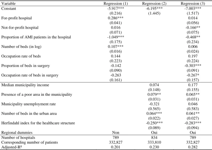
We then regress the hospital …xed e¤ects on a set of hospital and geographic variables. Results are reported in Table 5 (estimated regional dummies corresponding to the speci…cation of column 3 are reported in Appendix A3). When we only introduce hospital variables (column 1), the adjusted-R2

is quite low at 0:13.13 _{It is larger at 0:23 when only geographic variables enter the speci…cation}

13_{This adjusted-R}2 _{accounts for the sampling error and its formula is given in Gobillon, Magnac and Selod}

(column 2). Interestingly, when introducing both groups of variables (column 3), the R2 _{at 0:28 is}

below the sum of R2 _{of the two separate regessions (0:36), which suggests that variables are quite}

correlated. Also, it is higher than the R2 _{of each separate regression, which suggests that each of}

the two groups has some explanatory power of its own.

We now comment the sign of the estimated coe¢ cients for the full speci…cation (column 3). We …nd that the propensity to die is nearly the same in for-pro…t hospitals and public hospitals. This result may look surprising but it comes from the fact that we control for innovative treatments (mainly angioplasty and stent). If we drop the variables related to innovative treatments from the …rst-stage speci…cation, the propensity to die in public hospitals becomes higher than in for-pro…t hospitals (see Table A3 in appendix). Hence, the higher e¢ ciency of for-pro…t hospitals would come from a wider use of innovative treatments. We also …nd that the propensity to die in a NFP hospital is lower than in public or for-pro…t hospitals.

The proportion of patients in the hospital treated for an AMI has a negative and signi…cant e¤ect. It is possible that hospitals concentrating AMI patients are specialized in heart-related pathologies and thus have a higher e¢ ciency. The number of beds as well as their occupation rate have no e¤ect on mortality. The propensity to die is lower in hospitals with a higher proportion of beds in surgery (whether controlling for innovative treatments or not). In fact, hospitals with a high proportion of beds in surgery could be specialized in serious diseases and have a higher quality sta¤. The propensity to die also decreases with the occupation rate of beds in surgery (signi…cantly at 10% only). It is possible that hospitals with a high occupation rate are also those which are the more e¢ cient and the more likely to attract patients.

Among municipal variables, the presence of a poor area has a positive e¤ect (signi…cant at 10%) on the propensity to die, whereas the median income and the unemployment rate have no signi…cant e¤ect. The positive e¤ect of the presence of a poor area can be explained with a deterioted health of local people (the general health status being not captured with diagnoses variables).

The number of beds in the urban area has a positive signi…cant e¤ect which turns out to be negative but not signi…cant when innovative treatments are not controlled for. An interpretation can be that larger markets propose more innovative treatments but also yield more congestion. These two e¤ects would compensate but after controlling for the innovative treatments, only the congestion e¤ects would remain. The Her…ndahl index for the number of patients across hospitals computed at the urban area level has a signi…cant negative e¤ect. This result suggests that the fewer the hospitals in which patients are concentrated, the lower the propensity to die.

Finally, regional dummies always have a negative e¤ect compared to the reference (Languedoc-Roussillon) and their e¤ect is most often signi…cant. Di¤erences may be explained by unobserved regional factors such as the regional di¤erences in the propensity to transfer patients when they are likely to die. Indeed, recall that we work only on patients who come from their place of residence and not from a transfer. Note that standard errors are quite large and two regions should be far enough in the distribution of regional e¤ects for the di¤erent between their e¤ects to be signi…cant. The ranking of regional e¤ects is nearly uncorrelated with the probability to die within 15 days obtained from raw data (unweighted rank correlation: :02) and with that obtained from the model (unweighted rank correlation: :11).

[Insert T able 5]

We now perform a variance analysis at the regional level. Taking the logarithm of equation (1) under the multiplicative assumption (4), and computing the average for any region r gives:

1 Nr X ijj(i)2r ln (t_jXi; j (i) ) = X r + ln r+ (t)

where Nr_{is the number of patients in region r, X}r _{is the regional average of individual explanatory}

variables and ln r is the regional average of hospital …xed e¤ects weighted by the number of patients in the hospitals. It is possible to qualitatively assess the relative explanatory power of right-hand side terms computing their variance and their correlation with the left-hand side term (see Abowd, Kramarz and Margolis, 1999). In fact, the larger the variance and the correlation, the higher the explanatory power. In practice, as and ln r are not observed, we use their estimators b and dln

r

(the latter being de…ned as the weighted average of [ln j) to compute

the right-hande side terms. An estimator of the left-hand side term is obtained from the sum of right-hand side terms. Using the same approach, we also assess the explanatory power of Xr_sb for some sub-groups Xr_s of explanatory variables. Importantly, note that this procedure measures the explanatory power ex ante before any …ltering process of patients through tranfers or home returns. We can further assess the explanatory power of hospital and geographic variables. Taking the log of the expression of hospital …xed e¤ects and averaging at the regional level, we get:

ln r = Zr + r

where Zr and r_{are the regional averages of explanatory variables and random terms, respectively.}

We can assess the explanatory power of Zr and Zr_s , for some sub-groups Zr_s of explanatory variables, in the same way as for individual variables (replacing by its estimator).

We …nd that individual variables have a far larger power than hospital e¤ects in explaining re-gional disparities in mortality (see Table 6a). Indeed, their variance is …ve to six times larger. Interestingly, among the individual variables, it is the innovative treatments which have the largest explanatory power. This means that regional disparities in innovative treatments are a key fac-tor in explaining regional disparities in mortality. This has some important consequences for the regional funding of innovative equipments. Of course, the age-and-sex regional composition also plays a role. Interestingly, the hospital and geographic e¤ects have a larger variance than the composition e¤ects, which suggests that their role in explaining regional disparities is signi…cant. Note that the sum of variances for groups of individual variables is far smaller than their sum. This comes from fairly large correlations between groups. In particular, regions where patients are aged and mostly females are also those in which more innovative treatments are performed (correlation between the demographic e¤ects and the e¤ect of innovative treatments: :57).

When trying to explain regional disparities in hospital …xed e¤ects, we …nd that hospital variables do not have much explanatory power (Table 6b). In particular, the local composition of ownership status does not play much. By contrast, geographic variables have a large explanatory power. The local size of the market (measured by the local number of beds) and the local concentration of patients play a signi…cant role.14 This is not the case of municipality variables. Finally, residual local e¤ects captured by regional dummies have a large variance. This means that some regional unobserved factors have a large e¤ect on regional disparities in AMI death.

[Insert T able 6a and 6b] (8)

6

Conclusion

In this paper, we studied the regional disparities in mortality for patients admitted in hospitals for a heart attack. This was done using a unique matched patients-hospitals dataset over the 1998-2003 period constructed from exhaustive administrative records. For patients, this dataset contains some information on demographic characterics (sex and age), diagnoses and treatments. For hospitals, it gives some details on the location, the status, the mode of reimbursment and the

14_{Note that the local size of the market and the local concentration of patients have an e¤ect that is positively}

correlated with hospital …xed e¤ects. However, their correlation with the overall integrated hazard (last column in Table 6b) is negative. This is because these e¤ects are more than compensated by regional …xed e¤ects and the e¤ects of innovative treatments.

capacity.

We showed that regional disparities are fairly large. The di¤erence in the propensity to die between the extreme regions reaches 80%. We analyzed the causes of these disparities using a Cox duration model strati…ed by hospitals. This model allows for a speci…c hospital baseline hazard and controls for individual observed heterogeneity. Hence, it captures di¤erences in hospital behaviours when treating the patients. The survival functions of hospitals were averaged at the regional level to assess whether there are still some regional disparities after individual variables have been controlled for. Regional disparities decrease but remain signi…cant: the di¤erence in the propensity to die between the extreme regions is still 47%. Interestingly, the extent to which patients are treated with innovative procedures at the regional level plays a major role in the decrease of the disparities.

We then assessed to what extent the remaining regional disparities could be explained with the local composition of hospitals and geographic e¤ects. This was done regressing hospital hazards on hospital and geographic variables, and averaging the model at the regional level. We found that once treatments have been controlled for, hospital variables do not play much. By contrast, geographic variables, and in particular the local concentration of patients, play a signi…cant role. The more patients are concentrated in a few large hospitals rather than many small ones, the lower the mortality. After hospital and geographic variables have been controlled for, some signi…cant regional disparities still remain.

The scope of our analysis is limited because patients were not tracked in the data when they were transferred to another hospital. For patients who were transferred, we had to consider that the length of stay was censored. An interesting extension of our work would be to study the strategic behaviour of hospitals when transferring patients. Indeed, some hospitals may try to minimize their mortality rate by transferring the patients who are the most likely to die even when they are well equipped and can conduct some innovative treatments. Others, like local hospitals, may try to increase the propensity to survive of some patients by sending then to more e¢ cient establishments. It should be possible to conduct such an analysis in the future when data tracking patients (which exist) will be made available for research.

7

Appendix: second-stage estimation

In this appendix, we explain how to construct some estimators of the baseline hazard and hospital …xed e¤ects. We …rst average equation (4) across time, weighting the observations by the number of patients at risk at each date. We obtain:

1 N X t Nt j(t) = j 1 N X t Nt (t)

where Nt is the number of patients at risk at the beginning of period t, N =

P t Nt with P t the sum from 1 to T days (with T = 30 in the application). A natural identifying restriction is that the average of instantaneous hazards equals one: _N1P

t Nt (t) = 1. We obtain: j = 1 N X t Nt j(t) (9)

It is possible to construct an estimator of hospital …xed e¤ects from this formula, but weights (namely: Nt) are not hospital-speci…c and thus do not re‡ect hospital speci…cities. Hence, we

propose another estimator of hospital …xed e¤ects in the sequel which we believe better capture hospital speci…cities.

We also average equation (4) across hospitals, weighting by the number of patients at risk (summed across all dates) in each hospital. We get:

1 N X j Nj j(t) = 1 N X j Nj j ! (t) where Nj ₌ P t

Njt with Njt the number of patients at risk in hospital j at the beginning

of date t (such that N = P

j

Nj_{). Replacing}

j with its expression (9), we obtain: (t) = 1 N2 P j;t Nj_N t j(t) ! 1 1 N P j Nj j(t) !

. An estimator of the hazard rate at date t in hospital j can be constructed from the Breslow’s estimator such that bj(t) = bj(t) bj(t 1). A natural

estimator of the baseline hazard is then: b (t) = 1 N2 X j;t NjNtbj(t) ! 1 1 N X j Njbj(t) !

We then construct an estimator of a given hospital …xed e¤ect j averaging equation (4) across

day in this hospital. We obtain: 1 Nj X t Njt j(t) = j 1 Nj X t Njt (t)

An estimator of the hospital …xed e¤ect is then: bj = 1 Nj X t Njtb (t) ! 1 1 Nj X t Njtbj(t) ! (10)

We also computed the asymptotic variances of b = b (1) ; :::; b (T ) 0 and_{b = (b}1; :::;bJ)0, denoted

V et V , with the delta method. Indeed, the covariance matrix of bJ = b1(1) ; :::; bJ(T ) 0

can be estimated from Ridder et Tunali (1999). Its estimator is denoted bV _J. We can then compute the estimators: bV = @b @b0J b V _J @b0 @bJ and b V = @b @b0J b V _J @b0 @bJ . The vectors @b @bJ and @_b @bJ are given by: @b (t) @bk( ) = N N k P j;t Nj_N tbj(t) 1_{ft= g} N N k_N " P j;t Nj_N tbj(t) #2 X j Njb (t) (11) @_bj @bk( ) = _P Nk t Nj;tb (t) 1_{fk=jg b}j P t Nj;t_@b@b(t) k( ) P t Nj;tb (t) (12)

In practice, to simplify the computations, we neglected the second term on the right-hand side of (12). This is only a slight approximation that does not have much impact on the estimated variance of _bj. It amounts to neglect in (10) the variations of _N1j

P

t

Njtb (t) with respect to the

terms bj(t) compared to the variations of _N1j

P

t

Njtbj(t) which is far larger. Put di¤erently, b (t)

is supposed to be non-random in (10).

References

[1] Abowd M., Kramarz F. and D. N. Margolis (1999), “High wage workers and high wage …rms”, Econometrica, 67(2), pp. 251–333.

[2] Combes PPh., Duranton G. and L. Gobillon (2008), “Spatial Wage Disparities: Sorting Matters”, Journal of Urban Economics, 63, pp.723-742.

[3] Cutler D.M. and J.R. Horwitz (1998), “Converting Hospitals from Not-for-Pro…t to For-Pro…t States: Why and What E¤ects?”, NBER Working Paper no. 6672.

[4] Dormont B. and C. Milcent (2002), “Quelle régulation pour les hôpitaux publics français?”, Revue d’Economie Politique, 17(2).

[5] Dormont B. and C. Milcent (2006), “Innovation di¤usion under budget constraint. Micro-econometric evidence on heart attack in France”, The Annals of Economics and Statistics. [6] Duranton G. and V. Monastiriotis (2004), “Mind the Gaps: The Evolution of Regional

In-equalities in the U.K. 1982-1997”, 42(2), pp. 219-256.

[7] Etilé F. and C. Milcent (2006) “Income-related reporting heterogeneity in self-assessed health: evidence from France”, Health Economics, 15(9), pp. 965-981.

[8] Geweke J., Gowrisankaran G. and R. Town (2003), “Bayesian Inference For Hospital Quality in a Selection Model”, Econometrica, 71, pp. 1215-1238.

[9] Gobillon L., Magnac T. and H. Selod (2007), “The e¤ect of location on …nding a job in the Greater Paris Area”, CEPR Working Paper no. 6199.

[10] Gowrisankaran G. and R. Town (2002), “Competition, Payers, and Hospital Quality”, NBER Working Paper no. 9206.

[11] Hansman H.B. (1996), The ownership of Enterprise, Cambridge, Havard University Press. [12] Ho V. and B. Hamilton (2000), “Hospital mergers and acquisitions: Does market consolidation

harm patients?”, Journal of Health Economics, 19(5), pp. 767-791.

[13] Idler E.L. and Y. Benyamini (1997), “Self-rated health and mortality: a review of twenty-seven community studies”, Journal of Health and Social Behavior, 38, pp. 21-37.

[14] Jollis J., Peterson E., DeLong E., Mark D., Collins S., Muhlbaier L. and D. Prior (1994), “The Relation between the Volume of Coronary Angioplasty Procedures at Hospitals Treating Medicare Bene…ciaries and Short-Term Mortality”, The New England Journal of Medicine, 24(331), pp. 1625-1629.

[15] Kessler D. and M. McClellan (2002), “The e¤ects of hospital ownership on medical produc-tivity”, RAND Journal of Economics, 33(3), pp. 488-506.

[16] Lindeboom M. and M. Kerkhofs (2000), “Multistate Models for Clustered Duration Data - an Application to Workplace E¤ects on Individual Sickness Absenteeism”, The Review of Economics and Statistics, 82(4), pp. 668-684.

[17] Lindeboom, M. and E. van Doorslaer (2004), “Cut-point Shift and Index Shift in Self-reported Health”, Journal of Health Economics, 23, pp. 1083-1099.

[18] McClellan M. and D.O. Staiger (2000), “Comparing Hospital Quality at For-Pro…t and Not-for-Pro…t Hospitals”, in The Changing Hospital Industry: Comparing Not-Not-for-Pro…t and For-Pro…t Institutions, D.M. Cutler ed., University of Chicago Press.

[19] Milcent C. (2005), “Hospital Ownership, Reimbursement Systems and Mortality rates”, Health Economics, 14, pp. 1151–1168.

[20] Milcent C., Dormont B., Durand-Zaleski I. and P.G. Steg (2007), “Gender Di¤erences in Hospital Mortality and Use of Percutaneous Coronary Intervention in Acute Myocardial In-farction”, Circulation, 115(7), pp. 823-826.

[21] Mobley L.R. (2003), “Estimating hospital market pricing: an equilibrium approach using spatial econometrics”, Regional Sciencs and Urban economics, 49, pp. 489-516.

[22] Moulton (1990), “An Illustration of a Pitfall in Estimating the E¤ects of Aggregate Variables on Micro Units”, The Review of Economics and Statistics, 72(2), pp. 334-338.

[23] Newhouse J. (1970), “Toward a Theory of Nonpro…t Institutions”, American Economic Re-view, 60(1), pp. 64-74.

[24] Pauly M.V. and M. Redish (1973), “The Not-for-Pro…t Hospital as a Physicians’cooperative”, American Economic Review, 63, pp. 87-99.

[25] Propper C., Burgess S. and K. Green (2004), “Does competition between hospitals improve the quality of care? Hospital death rate and the NHS internal market”, Journal of Public Economics, 88(7-8), pp. 1247-1272.

[26] Ridder G. and I. Tunali (1999), “Strati…ed partial likelihood estimation”, Journal of Econo-metrics, 92(2), pp. 193-232.

[27] Silverman E.M.and J.S. Skinner (2001), “Are For-Pro…t Hospitals Really di¤erent? Medicare Upcoding and Market Structure”, NBER Working Paper no. 8133.

[28] Sloan F., Picone, G., Taylor D. and S. Chou (2001), “Hospital Ownership and Cost and Quality of Care: Is There a Dime’s Worth of Di¤erence?”, Journal of Health Economics, 20(1), pp. 1-21.

[29] Van Doorslaer E., Wagsta¤ A., Bleichrodt H. , Calonge S., Gerdtham U.G., Ger…n M. , Geurts J., Gross L., Häkkinen U., Leu R., O’Donnell O., Propper C., Pu¤er F., Rodriguez M., Sundberg G. and O. Winkelhake (1997), “Socioeconomic inequalities in health: some international comparisons”, Journal of Health Economics, 16(1), pp. 93-112.

[30] Van Doorslaer E., Wagsta¤ A., van der Burg H., Christiansen T., Citoni G., Di Biase R., Gerdtham U., Ger…n M., Gross L., Häkkinen U., John J., Johnson P., Klavus J., Lachaud C., Lauritsen J., Leu R., Nolan B., Perán E., Pereira J., Propper C., Pu¤er F., Rochaix L., Rodriguez M., Schellhorn M., Sundberg G. and O. Winkelhake (1999), ”The redistributive e¤ect of health care …nancing in 12 OECD countries”, Journal of Health Economics, 18, pp. 291-313.

[31] Van Doorslaer E., Wagsta¤ A., van der Burg H., Christiansen T., De Graeve D., Duchesne I., Gerdtham U.G., Ger…n M., Geurts J., Gross L., Häkkinen U., John J., Klavus J., Leu R.E., Nolan B., O’Donnell O., Propper C., Pu¤er F., Schellhorn M., Sundberg G., Winkelhake O. (2000), “Equity in the delivery of health care in Europe and the US”, Journal of Health Economics 19(5), pp. 553-583.

Table 1: disparity indices

for the regional averages of individual variables

Mean Min Max Max/Min Std. Dev. Coeff. of

variation Gini

Number of AMI patients 21448 6335 44393 7.008 11534 0.538 0.295

Death 0.080 0.059 0.098 1.675 0.0098 0.123 0.070

Female, 35-55 year old 0.024 0.015 0.032 2.145 0.0050 0.207 0.117

Female, 55-65 year old 0.026 0.021 0.034 1.609 0.0031 0.117 0.066

Female, 65-75 year old 0.072 0.060 0.089 1.475 0.0074 0.103 0.056

Female, 75-85 year old 0.109 0.093 0.134 1.435 0.0100 0.092 0.050

Female, more than 85 year old 0.087 0.059 0.110 1.852 0.0126 0.144 0.081

Male, 35-55 year old 0.187 0.135 0.239 1.771 0.0291 0.155 0.088

Male, 55-65 year old 0.139 0.116 0.158 1.372 0.0137 0.099 0.057

Male, 65-75 year old 0.175 0.145 0.195 1.343 0.0139 0.079 0.042

Male, 75-85 year old 0.134 0.105 0.159 1.510 0.0172 0.129 0.074

Male, more than 85 year old 0.046 0.027 0.062 2.259 0.0090 0.196 0.108

Excessive smoking 0.120 0.062 0.196 3.160 0.0350 0.293 0.164 Alcohol problems 0.012 0.004 0.017 4.148 0.0029 0.248 0.137 Obesity 0.063 0.018 0.111 6.273 0.0196 0.313 0.170 Diabetes mellitus 0.155 0.092 0.208 2.254 0.0240 0.156 0.077 Hypertension (MH) 0.299 0.203 0.373 1.833 0.0369 0.123 0.067 Renal failure 0.050 0.028 0.078 2.760 0.0085 0.171 0.088 Conduction disease (TC) 0.197 0.134 0.247 1.843 0.0218 0.111 0.060

Peripheral arterial disease (AR) 0.063 0.036 0.109 3.019 0.0145 0.231 0.113

Vascular disease (VC) 0.044 0.025 0.078 3.109 0.0108 0.248 0.128

History of coronary artery disease (COEUR) 0.040 0.017 0.070 4.000 0.0100 0.250 0.134

Stroke (CER) 0.032 0.020 0.048 2.448 0.0055 0.173 0.092

Heart failure (IC) 0.158 0.128 0.204 1.598 0.0184 0.116 0.064

Severity index (IGS) 0.283 0.143 0.438 3.054 0.0737 0.261 0.147

Cabbage or Coronary Bypass surgery (CABG)

0.009 0.001 0.036 36.312 0.0068 0.740 0.372

Cardiac catheterization 0.190 0.130 0.271 2.081 0.0347 0.182 0.100

Percutaneous transluminal coronary Angioplasty

0.054 0.010 0.106 10.914 0.0270 0.497 0.277

Other dilatation than PTCA 0.002 0.000 0.005 \ 0.0016 0.994 0.534

Percutaneous revascularization using coronary stents (PCI – stenting)

0.245 0.107 0.411 3.836 0.0909 0.372 0.206

Surgical French DRGs (GHMC) 0.037 0.016 0.077 4.650 0.0154 0.418 0.232

Source: computed from the PMSI dataset (1998-2003). Observed used to construct the disparity indices are weighted by the number of AMI patients.