Université de Montréal
Algorithms for Classifying Recorded Music by Genre
par James Bergstra
Département d’Informatique et de Recherche Operationelle Faculté des arts et des sciences
IVlémoire présenté à la Faculté des études supérieures en vue de l’obtention du grade de Maître ès sciences (M.Sc.)
en Informatique
Août, 2006
0i1
u
de Montréal
Direction des bibliothèques
AVIS
L’auteur a autorisé l’Université de Montréal à reproduire et diffuser, en totalité
ou en partie, par quelque moyen que ce soit et sur quelque support que
ce
soit, et exclusivement à des fins non lucratives d’enseignement et de
recherche, des copies de ce mémoire ou de cette thèse.
L’auteur et les coauteurs le cas échéant conservent la propriété du droit
d’auteur et des droits moraux qui protègent ce document. Ni la thèse ou le
mémoire, ni des extraits substantiels de ce document, ne doivent être
imprimés ou autrement reproduits sans l’autorisation de l’auteur.
Afin
de
se
conformer
à
la
Loi
canadienne
sur
la
protection
des
renseignements personnels, quelques formulaires secondaires, coordonnées
ou signatures intégrées au texte ont pu être enlevés de ce document. Bien
que cela ait pu affecter la pagination, il n’y a aucun contenu manquant.
NOTICE
The author of this thesis or dissertation has granted a nonexciusive license
allowing Université de Montréal to reproduce and publish the document, in
part or in whole, and in any format, solely for noncommercial educational and
research purposes.
The author and co-authors if applicable retain copyright ownership and moral
rights in this document.
Neither the whole thesis or dissertation, nor
substantial extracts from it, may be printed or otherwise reproduced without
the author’s permission.
In compliance with the Canadian Privacy Act some supporting forms, contact
information or signatures may have been removed from the document. While
this may affect the document page count, it does flot represent any loss of
content from the document.
Ce mémoire intitulé:
Algorithms for Classifying Recorded Music by Genre
présenté par:
Jarnes Bergstra
a été évalué par un jury composé des personnes suivantes: Yoshua Bengio, président-rapporteur
Douglas Eck, directeur de recherche Sébastien Roy, membre du jury
Résumé
Ce mémoire traite le problème de la classification automatique de signaux musicaux par genre. Dans un premier temps, je présente une technique utilisant l’apprentissage machine pour classifier des statistiques extraites sur des segments du signal sonore. IVIalgré le fait que cette technique a déjà été explorée, mon mémoire est le premier à investiguer l’influence de la longueur et de la quantité de ces segments sur le taux de classification. J’explore également l’importance d’avoir des segments contigus dans le temps. Les segments d’une à trois secondes apportent une meilleure performance, mais pour ce faire, ils doivent être suffisamment nombreux. Il peut même être utile d’augmenter la quantité de segments jusqu’à ce qu’ils se chevauchent. Dans les mêmes expériences, je présente une formulation alternative des descripteurs d’audio nommée IViel frequency Cepstral Coefficient (MFCC) qui amène un taux de classification de 81
¾
sur un jeux de données pour lequel la meilleure performance publiée est de 71%.
Cette méthode de segmentation des chansons, ainsi que cette formulation alternative, ont pour but d’améliorer l’algorithme ga gnant du concours de classification de genre de MIREX 2005, développé par Norman Casagrande et moi. Ces expériences sont un approfondissement du travail entamé par Bergstra et al. [2006a], qui décrit l’algorithme gagnant de ce concours.Dans un deuxième temps, je présent une méthode qui utilise freeD3, une base de données d’information sur les albums, pour attribuer à un artiste une distribution de probabilité sur son genre. Avec une petite base de données, faite à la main, je montre qu’il y a une haute corrélation entre cette distribution et l’étiquette de genre traditionnel. Bien qu’il reste à démontrer que cette méthode est utile pour organiser une collection de musique, ce résultat suggère qu’on peut maintenant étiqueter de grandes bases de musique automatiquement à un faible coût, et par conséquent de poursuivre plus facilement la recherche en classification à grande échelle. Ce travail sera publié comme Bergstra et al. [200Gb] à ISMIR 2006.
Keywords: classification de musique par genre, extraction de caractéristiques sonores, recherche d’information musicale, apprentissage statistique
Abstract
This thesis addresses the problem of how to classify music by genre automatically. First, I present a technique for labelling songs that uses machine learning to classify summary statistics of audio features from multiple audio segments. Though this technique is not new, this work is the flrst investigation of the effect of segment length and number on classification accuracy. I also investigate whether it is important that the segments be contiguous. I find that one- and three-second contiguous segments perform best as long as there are sufficiently many segments, and it helps to use more segments than are necessary to cover the song by letting them overlap. In the same experiments, I present an alternative formulation of the popular Mel-frequency Cepstral Coefficient (IVIFCC) audio descriptors that leads to 81% classification accuracy on n public dataset for which the highest published score is 71%. This segmentation method and new audio feature are both improvements on an algorithm by Norman Casagrande that won the MIREX 2005 genre classification contest. These experiments follow directions for future work proposed in Bergstra et al. {2006a], which describes the contest-winning algorithm.
Second, I present a technique for distilling artist-wise genre descriptors from an online CD database called FreeDB. Using a small hand-made dataset, I show that these descriptors are highly correlated with traditional genre labels. While it remains to be seen whether these descriptors are suitable for organizing music collections, this result raises the possibility of automatically labelling large datasets at low cost, thereby spurring research in large-scale genre classification. This work will be published as Bergstra et al. [200Gb] in the proceedings of ISMIR 2006.
Keywords: music genre classification, audio feature extraction, music information retrieval, machine learning
1 Introduction 13 1.1 Contribution 13 1.2 Layout 14 2 Background 15 2.1 IViusic Genre 15 2.1.1 Traclitional Genre 16 2.1.2 Collaborative Genre 17 2.2 Sound 18
2.2.1 Physics and Perception of Sound 18
2.2.2 Signal Intensity 18
2.2.3 Decibels. Phons 19
2.2.4 Loudness 19
2.2.5 Critical Bands. Mel Scale 19
2.2.6 Discrete Fourier Transforrn 19
2.2.7 Cepstral Analysis 20
2.2.8 Summary 21
2.3 Machine Learning of Multiclass Classifiers 21
2.3.1 Model Evaluation, Selection 22
2.3.2 Neural Networks 23
2.3.3 Other Classifiers 25
3 Genre Classification Datasets 27
3.1 Tzanetakis 27
3.2 AilMusic 28
3.3 USPOP 29
3.1 MIREX 2005 29
3.5 freeDB 30
3.5.1 Tags per Track 31
3.5.2 Overail Tag Popularity 31
3.5.3 first-Tag Importance 33
3.6 LastfM . 34
4 Genre Classification of Recorded Audio 35
4.1 Frame-level Features to Represent Music 36
4.1.1 FFTC 36
4.1.2 RCEPS 37
4.1.3 MFCC 38
4.1.4 ZCR 39
4.1.5 Rolloif 39
4.1.6 Spectral Centroid, Spectral Spread 40
4.1.7 Autoregression (LPC, LPCE) 40
4.2 Song Classification Algorithms 41
4.2.1 No Aggregation 41
4.2.2 Feature Sample Statistics 41
4.2.3 Song Segmentation 41
4.2.4 Mixture Modelling 41
4.2.5 Rhythm, Temporal Dynarnics 42
4.3 Contiguous and Non-Contiguous Song Segmentation 42
4.4 Mel-Scale Phon and Sone Coefficients 43
1.5 Neural Network Classifier 44
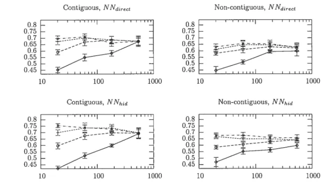
1.6 Feature and Segmentation Performance 44
4.6.1 Mel-scale Cepstral Coefficients 46
4.6.2 MIREX.MV 47
4.6.3 Mel-scale Phon Coefficients 48
4.6.4 Mel-scale Sone Coefficients 48
4.6.5 Analysis 49
4.7 Discussion 51
5 Genre Classification of FreeDB Histograms 52
5.1 Input: FreeDB 52 5.2 Target: AllMusic 53 5.3 PredictiveModel 54 5.4 Prediction Performance 54 5.4.1 Classification Rates (1 — L0— 1) 54 5.4.2 KL Divergence 55 5.5 Discussion 56
6 Future Work and Conclusion 57
6.1 Coarse Genre Classification 57
6.2 High-Resolution Genre Classification . 57
Bibliography 60
A Software 64
A.1 fextract 64
A.2 liblayerfb 64
B Last.FM Tag Sample 66
3.1 Tzanetakis summary 27
3.2 AlliViusic Genre I-Iierarchy 28
3.3 USPOP summnry 29
3.4 MIREX 2005 dataset surnmary 30
3.5 MIREX 2005 Genre contest resuits 30
4.1 Feature surnmary; MIREX.IVIV 46
5.1 Predictive power of FreeDB genre histograms 54
3.1 Histogram of Genres-per-Track for FreeDB 32
3.2 Histogram of Tag Frequencies 32
3.3 Histogram of First-Tag Importance on FreeDB 33
4.1 Pseudocode: IViel-Scale Warp 38
4.2 Pseudocode: Zero-Crossing Count without fPU 39
4.3 Contiguous Segmentation 42
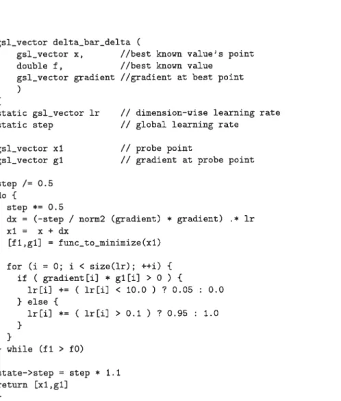
4.4 Pseudocode: Delta-bar-Delta 45
1.5 The performance of the MFCC.IVICV features 47
4.6 The performance of the IVIIREX.MV features 8
4.7 The performance of the MPC.MCV features 49
4.8 The performance of the MSC.MCV features 50
5.1 Examples of FreeDE-genre 53
5.2 Ranking of Alliviusic-genre 56
List of Abbreviations
DFT Discrete Fourier Transform
IVIFCC IVIel-frequency Cepstral Coefficients
MIREX Music Information Retrieval Evaluation Exchange PCM Pulse Code Modulation
RCEPS Real Cepstral Coefficients
cla.ss (in context of classification) G a set of classes
s a feature vector X a feature vector space dct() Discrete Cosine Transform
F3 Discrete Fourier transform of signal
s
f A rnulticlass predictorI Intensity (of a signal)
Indicator function. Y if cond is true, O otherwise k Frequency, used as an index
KL Kullback-Leibler divergence L Loudness, in Phons
L0_1 O-1 Loss over a population Lmjn Training error
L1 Validation error Ltest Test error
Lo—;
O-1 Loss over a finite sample t Learning Algorithmp Pressure (of a signal)
p A discrete probability mass function The probability assigned by p to event j q A discrete probability mass function q The probability assigned by p to event j R A Training Set
S A dataset of (feature: class) pairs
s
SignalSarnpled Signal T Time, used as a bound
T Test Set
Acknowledgemellts
I would like to thank several students and professors in the GAMME and USA labs, whose ideas and encouragement inspired me: Norman Casagrande, Alexandre Lacoste, Dumitru Erban, Balazs Negi, and Yoshua Bengio.
I would like to thank Douglas Eck for bis pragmatic guidance, and also for affording me the freedom to experiment. Many of the things I tried did not make it into tbis document, but some of them did, and it kept the Masters fun.
I would like to thank O1’ga on a personal level for ber patience, impatience, and support, and on a technical level for her careful proofreading and numerous suggestions for the text.
I would like to thank my family for their support and understanding (especially on Thanks giving 2005).
I would like to tbank Benoit for renting us bis beautiful apartement on Rue Jean Maridor this past July.
Introduction
This Masters thesis addresses the problem of how to classify recorded music by genre automat ically. Provisionally, consider that a genre is a set of similar-sounding musical works. Genre descriptors constitute an important navigational mechanism for music collections. The right genre descriptors can help individuals browse their own collections, but more irnportantly they can help listeners to search efficiently through the enormous quantity of music that is currently available (online, for example) without listening to it. As automatic collaborative and content based indexing tools improve, individuals are empowered to circumvent the record publishing industry and connect directly with the artists they support. Not only can such tools help music fans find better music, they can help budding artists find an audience.
1.1
Contribution
This Masters thesis contributes to the project of automatic genre labelling in two ways. First, it presents a new song classification algorithm that is better than previously published ones on n public dataset. The advances are in the areas of feature extraction and of song segmentation (explained in chapter 4). A variation of this algorithm was the best genre classification algorithm at MIREX 2005, an annual music information retrieval competition conducted in conjunction with the ISMIR conference. Several variations of the technique are evaluated in chapter 4.
Second, this thesis contributes a technique for using a previously unused online repository of CD meta-data as a resource for automatically labelling artists with n genre descriptor. This genre descriptor is a broad multinomial probability distribution, but chapter 5 shows that there is a strong correlation between this notion of genre and a more traditional one from AMG (http: //www.allmusic.com). It remains to be seen whether this notion of genre cnn identifv similar tastes of music fans, but experiments with AMG’s data show that it is a reasonnable surrogate for truc genre labels in the context of developing and evaluating automatic genre-classification algorithms.
1.2
Layout
This document is arranged as follows.
Chapter 2 covers required background material including discussion of what music genre is, a basic primer in the physics, perception, and processing of sound, and a brief introduction to the principles and methods of machine learning.
Chapter 3 describes datasets that represent music genre learning problems.
Chapter 4 is the first chapter of original work, in which I present and evaluate some algorithms for classifying recorded music. It should be viewed as a follow-up to Bergstra et al. [2006aj, which is attached as appendix C. This chapter includes a lengthy discussion of acoustic features for classification and details of their implementations.
Chapter 5 is the second chapter of original work, in which I evaluate a collaborative online CD catalog as an alternative to a traditional (but expensive) online music reference. This chapter borrows heavily from Bergstra et al. [2006b].
Chapter fi presents some directions for future work, and conclusions to be drawn from chapters 4 and 5.
Appendix A describes some of the more interesting software written in the course of my IViasters: a library for extracting audio features, and a library for implernenting neural networks. Appendix B lists a random sample of tags from the LastFM dataset.
B ackground
In this section I introduce the topics of music genre, physics and psycho-acoustics of sound, the fourier Transform, and machine learning. The section on music genre will prepare the reader for chapter 3, in which I present severai types of genre datasets. The section on sound wiil provide sorne theoretical basis for the audio feature-extraction aigorithms presented in chapter 4. The section on machine learning (with n focus on fleurai networks) provides some background on the methodoiogy applied in chapters 4 and 5, as well as previous work in genre classification.
2.1
Music Genre
“Genres are tools used to commodify and commercialize an artist’s complex personal vision.”
-John Zorn
There are rnany perspectives on what music genre is, and how genre classification shouid be approached. For example, Pachet and Cazaly [2000] introduced n genre hierarchy that uses instrumentation and historicai descriptors. Other researchers such as McKay and Fujinaga [2005] have defined self-consistent and compiete taxonomies for the purposes of classifying music without ambiguity. 1-Iowever, these can be seen as aiternatives to a mainstream view of genre that is embodied in terms like rock, btnes, and pop. In this section, I present two views of genre that posit music genre descriptors as mechanisms for music recommendation, rather than detaiied or consistent classification. What I will refer to as traditionat genre is the one deveioped by the record pubiishing industry primarily for product placement. What I will refer to as cottaborative genre arises from oniine databases in which a large number of listeners apply their own labels.
2.1.1
Traditional Genre
AviG’s AilMusic Guide, a large and influential reference for music genre, arranges genre labels in a simple two-level hierarchy.’ At the top level, they have ctassicatand poputar, beneath which we find genres like ballet, con certo, sijmphony and blues, rap, tatin, respectively. AllIViusic is described in more detail in section 3.2, but it should be understood that these genres are very broad both in terms of style and appeal. To provide more descriptive power within the restrictive hierarchy, AilMusic bas introduced “Style” and “Mood” descriptors to the songs, albums, ancl artists in their database. The genre list that vas part of the 1D3 standard is another well-known list.2 The original 1D3 standard provided a single numerical field within each tag to record the genre to which the recording belonged. This list was similar in spirit to AllMusic’s taxonomy, though the specific choice of genres vas different.
Since artists do not mention genres in their creations, it is interesting to consider where genres come from. One explanation, articulated by Perrott and Gjerdingen [1999], is that the record publishing industry encouraged genres as a simple means to describe their different artists and acts. The broad genres such as rock and blues mentioned above can be seen in this light as components of a general method of music recommendation. There is no reason to suppose a priori that such genres serve as a taxonomy for music; indeed there is considerable evidence tha.t popular genre sets make poor taxonomies. Pachet and Cazaly [2000] outline a number of problems associated with using musical genres common in the music industry; Aucouturier and Pachet [20031 summarize:3
1. They are designed for albums, not tracks.
2. There is considerable disagreement among different taxonomies on how to classify individual albums.
3. Within these taxonomies, taxons do flot bear flxed semantics, leading to ambiguity and redundancy. (eg. Genres jazz and christmas overlap.)
4. They are sometimes culture-specific, and often flot related to actual musical content. (eg. A genre such as christian.)
Despite theoretical reasons for why genres are not taxonomies, genre papers from ISMIR proceedings (e.g. Fingerhut [2002] - Crawford and Sandler [2005]) have universally treated the
problem as one of classification. The target class sets have been of a small size, such as five to ten genres. If it seems like an artificially simple task, consider that it is at least one at which people are relatively good. If computers could represent the recordings in a suitable way, then it would be easy for computer programs too. The USPOP dataset (described in section 3.3) and a hand-labelted dataset using 10 genres according to George Tzanetakis (described in section 3.1) have been popular datasets for comparing algorithms. In both of these datasets, the genre groups are very coarse, and of limited value for making recommendat.ions.
‘Al]lvlusic is described more thoroughly in section 3.2
21D3 is a standard for embedding meta-information in mp3 audio. For details see http://www.id3.org. 3The examples have been added by the authors, tve hope that they are consistent with the original intent.
It should be borne in mmd throughout this thesis that genre classification, on its own, is not n relevant practical problem. As long as the number of genres is small, and defined by a
few human experts, it is flot difficuit for those experts to label new music on demand. While research in genre classification lias resulted in interesting algorithrns and audio representations for music classification, the final rneasure of these algorithms and representations must corne from elsewhere.
2.1.2
Collaborative Genre
An emerging alternative to the traditional view of genre cornes from Internet-based services such as FreeDB (the subject of chapter 5) and Last.FM (disdussed in section 3.6. FreeDB operates as a tagging service for CDs, and Last.FM operates customized radio streams for individual clients. Both of these services collect anonymous suggestions for the genre of specific albums or tracks, and do flot constrain suggestions to any sort of menu. Wherever one user attaches one genre, another user may attacli another and the system retains both labels. Songs, albums, and artists accumulate histograms over the growing number of labels in the system. The result is that these services have thousands of labels, though the labels aren’t organized into any hierarchy. These labels overlap, there is no atternpt at taxonomy. Some labels are broad, some narrow, sorne labels are words that have a meaning related to the music, the artist, the region or period of recording, and many labels in Last.FM’s collection have amusing meanings in English that are flot necessarily related to the music at all (e.g. pancakeday, wiggidywopwoo. See appendix B for a random sample of lastfrn tags.).
On one hand, we may see this histogram as quantifying uncertainty in the true genre of a particular song or artist; but on the other hand, we may see the histograrn as actually being a point in a continuous vector space of genre. These are both interesting possibilities that lead to subtly different learning problems. In the former case, the idea that there is a true genre suggests that a multiclass classification algorithrn would be appropriate. In the latter interpretation, a regression into multinomial parameters would be more natural.
Last.FM uses their labels as agents for recommendation, just like AllMusic, but Last.FM does not choose the genres or constrain their meaning as they evolve. Last.FM’s Tag Radio service plays the set of music with a certain tag as a radio station. Playing rock selects a very broad set of music, but srnaller genre sets such as etectropop generate very coherent radio, similar to the playlist of a specialty radio show. The large number of labels and semantics in this distributed notion of genre poses several problems, because no single person can label a new artist, album, or song to inject it into an established collection. In a nutshell: it is impossible to hear a new song on Tag Radio, because many people must listen to it (and tag it) first. Another problem is that it can be important to balance the relative strength of n song’s mernbership in different genres; a simple member vs. no-member decision is not natural. Furthermore, the lack of a natural hierarchy in flic label set means that tracks with only a specialized label cannot lie automatically included into more general labels’ sets. Learning to predict genre as n collaborative distribution is n difficult and relevant learning problem that is closely related to the learning problem associated with genre
as a taxonomy, but which introduces new challenges in data-mining and computational efficiency. This topic will be revisited in chapter 5, in which I evaluate the correspondance between freeDB and AflMusic, but many questions remain for future work (chapter 6).
2.2
Sound
This section begins with a brief survey of relevant topics in physics, psychoacoustics and signal processing, in preparation for discussion of audio feature extraction in chapter 4. This section is paraphrased from Cold and Morgan [2000], an introduction to signal processing and machine learning for speech analysis and synthesis. This background information motivates some of the standard transformations that extract features from audio for music classification, as well as the two features that wlll be introduced in chapter 3.
2.2.1
Physics and Perception of Sound
The basic premise of the physics of sound is that sound can be seen as a superposition of waves of different frequency, phase, and amplitude. Physically, sound is transmitted through air as oscillations in pressure with respect to time and space. Sound is transcribed to and from electric current using the same electro-mechanical device: a diaphragm attached to a magnet housed in a spool of insulated wire. In a microphone, oscillations in air pressure pull and push on the diaphragm and generate alternating current in the wire. In a loudspeaker, the reverse process uses alternating current in the vire to drive the diaphragm to create oscillations in air pressure. A digital sound signal is obtained by frequently and regularly measuring (sampting) the voltage on the wire from the microphone. The encoding of an audio signal by writing the values of these voltage samples is called Pulse Code Modulation (PCM). It is the encoding of sound that is used in .wav files, .au files, and CD-audio. CD audio, for example, is sampled at 44100FIz (Hertz, or 1-Iz, denotes a number of events per second).
2.2.2
Signal Intensity
Intensity is deflned as the amount of energy flowing across a unit area surface in a second. This is equivalent to the pressure p multiplied by the velocity y. The equation 2.1 shows how intensity
I relates to pressure p and velocity u. Under normal conditions (of low-amplitude waves) the velocity of air molecules varies linearly with the root-mean-squared (RMS) sound pressure. In this case the intensity I is proportional to the square of the pressure p.
I=pooci2 (2.1)
In this document, the terms pressure and intensity will always denote their respective RMS definitions.
2.2.3
Decibels, Plions
Decibels mensure the difference in energy between two signais. The definition of decibels, L, in equation 2.2 can be expressed either in terms of intensity or pressure, but in both cases a reference intensity or pressure is required.
L 101og10 —— = 201og10 --— (2.2)
‘ref ?ref
This iogarithmic energy scale is aiso used as a guide to the perceptual sense of loudness. Using n particular reference intensity ‘ref, this is referred to as the Phon scale.
2.2.4
Loudness
Another mensure of loudness is the sone, S. Empiricai work suggests that for pure tones (sound consisting of a single frequency), the sense of loudness is consistent with equation 2.3. In equation 2.3 S varies hnearly with the sone scale, p denotes pressure and I denotes intensity.
s
103 (2.3)The constant of proportionality in equation 2.3 depends on the frequency of the wave in question, which gives rise to so-called eqeat tondness curves, that give equivaient ioudnesses in terms of intensity at different frequencies. In general however, tones are not pure and the sense of loudness of n sound depends not only on their own intensity and frequency, but aiso the intensity and frequency and reiative phase of other tones in the signai. The importance of loudness transformations in feature extraction for music information retrieval was the subject of Lidy and Rauber [2005], and many genre classification algorithms published in the last few years use some form of ioudness transformation. See Gold and Morgan [2000] for more details on the perception of loudness.
2.2.5
Critical Bands, MeT Scale
Another important psycho-acoustic influence is the way pitch is perceived. The Mel-scale is a psycho-acoustic frequency scale on which n unit change carnes the same perceptual significance over the entire scale. This contrasts with the simpie Hertz scale. Whiie it is easy to differentiate two tones at 440Hz and 4411-Iz, it is much more difficuit to differentiate 44001-Iz from 4401Hz. The Mel-scaie increases identicaily with Hertz from O to 1000Hz, at which point it continues to rise iogarithmicaily while maintaining n continuous derivative. The effect is that a fixed precision on the Mei-scaie gives excellent resolution at low frequency, and coarse resolution of higli frequencies.
2.2.6
Discrete Fourier Transform
To paraphrase the Fourier Theorem, any periodic signal can be expressed as a sum of sinusoidal components of various frequencies, each with a certain phase. The Fourier Transform is the
transform that teils us, for a given signals, the amplitude and phase of the sinusoidal component at each frequency. Unfortunately, when working with audio, we have only a finite number of regularly-spaced samples of the true signal, so the truc fourier Transform does not apply. Instead, we defer to the Discrete Fourier Transform (DFT) given in equation 2.4, in which k is a frequency index, t is a sample (time) index running from O to sorne upper bound T, and ê is our sampled signal.
5[k] ê[t] (cos(2%) -isin(2x)) (2.4)
Note that in the DFT, we only measure the amplitude and phase of frequencies indexed by k. k may run from O to any positive upper bound, but an interesting effect will be observed. Consider that we can use k to indexa signalck from equation 2.4 whose t’th value is Ck[t] = cos(2x). After k passes half the sample-length (T) of the signal then a curious thing happens to êk: it appears to
be a sinusoid with lower and lower frequency. The cuiprit is the sampling frequency—the sinusoid oscillates too fast to be accurately measured—and the consequence is that T/2+a CT/2_a for
any integer n (assuming T is even). For this reason, we say that an audio signal of length T lias a Nyquist position of T/2, or alternately that an audio signal sampled at r Hz has a Nyquist frequency of r/2. A digital approximation of the original signal cannot record frequencies above the Nyquist frequency, and records frequencies approaching the Nyquist with reduced fidelity. As a corollary, it can lie seen that the frequency indexed by a given k is related to the Nyquist frequency of the signal. If the Nyquist frequency of the signal is rnyqHz, then the k’th frequency
2kr,,
is
In terms of the acoustic wave that ê represents, the result of the DFT transform is a vector of complex values, fk, that represents the amount and phase of energy at cadi of the T/2 indexed frequencies. The energy (intensity) observed in the k’th frequency over the length of the frame is the scalar value fkJ2. Similarly, the intensity observed in the k’th frequency interval is fk.
Almost all acoustic features for music classification are based on the magnitudes fk, although
3db et al. [20051 has shown that the phase component can be just as effective for detecting note onsets.
The discrete cosine transform (DCT, or in equations, dctQ) is a name for a DFT in which all imaginary components in the output are discarded. A more formal treatment of discrete and continuous signal analysis is given in Alan W. Oppenheim [1996].
2.2.7
Cepstral Analysis
Cepstral analysis is a technique developed especially for speech recognition, for quantitatively describing the quality of voiced sound. The technique is to compute the DFT of a short segment of audio (as short as 2Oms) in which a hurnan voice is speaking; to compute the loudness (on Phon scale, for example) of each complex element of the DFT (signal energy); and to perform a second DFT on the vector of boudness values. The two DFTs play subtly different roles. The first DFT (of the recorded signal) decomposes the utterance into its spectral components 50
seem strange because the basis of sinusoids lias no naturai semantics when applied to a vector of loudness values, as it does when applied to a signal of recorded audio. Nevertheless, the second DFT lias the effect of isolating descriptors of the general shape of the loudness vector in a few dimensions corresponding to low-frequency sinusoids. Furthermore, the number (and meaning) of low-frequency descriptors is independent of the resolution of the loudness vector (given the Nyquist frequency of the original recording). In speech recognition, the general shape of the loudness vector is very helpfui in predicting the shape of the mouth, and phone (unit of pronunciation) being produced. Real Cepstral coefficients (RCEPS) are the real components of the complex vector resulting from the second DFT.
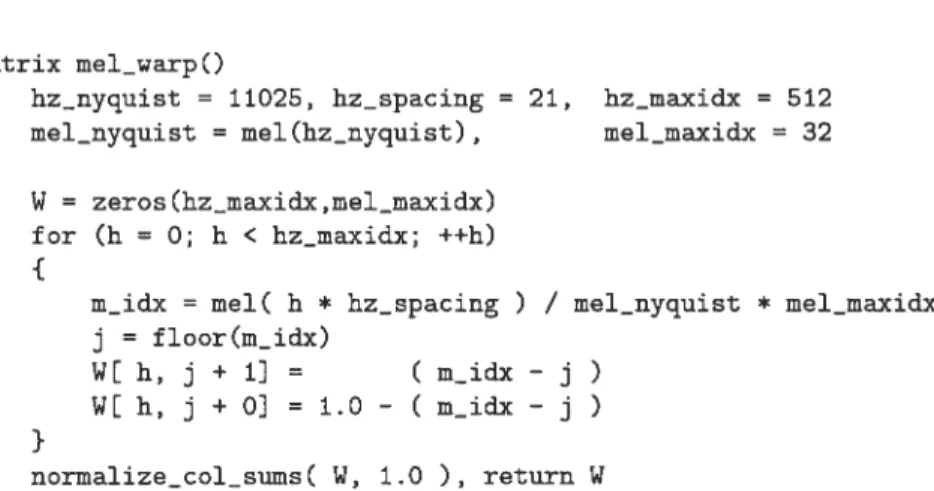
One variation on the method presented above adds a linear transformation of the DFT before adjusting for loudness. For example, the MeiScale Frequency Cepstral Coefficients (MFCC) are computed by averaging wider and wider frequency ranges according to the Mel scale. Numerous engineering tricks are often used to tweak this general recipe for speech recognition, and there is no one correct implementation of this method.4
For more information on Cepstral analysis sec Gold and Morgan t2000].
2.2.8 Summary
In this section, I presented a number of topics in physics and psycho-acoustics. These topics comprise motivation and some theoretical basis for the frame-level acoustic features that will be presented in chapter 4.
2.3
Machine Learning of Multiclass Classifiers
In this section, I present some of the basics of machine learning, in the context of multiclass classification. I begin with the formai setup of the classification probiem, and move on to methods of model evaiuation and seiection. I describe neurai networks, the particuiar class of predictor that 1’li use in my own experiments, and briefly describe some other classes of predictors such as decision trees, kernel machines, and probability models that are used in previous work. This contents of section are key to understanding the methodology of the experiments in chapters 4 and 5.
The basic premise of a multiclass classification problem is that there is some underiying plie nomenon that we can model reasonabiy weii as a joint probabihty distribution of examples that have both features x from some set of possible features X and classes c from a fuite set of possibilities C. This distribution gives risc to the conditionai probability P(c = CIx = X). Ma
chine learning of a multiclass classifier is the problem of guessing (learning) a predictor (machine)
f
: X — C that predicts the mode of this conditional probability distribution, when we have asample S of exampies x,c. A procedure that guesses a predictor is called a tearning atgorithm.
Throughout this document, the sample S wili be referred to as a dataset.
2.3.1
Model Evaluation, Selection
Before I can define model evaluation and model selection, I must explain the important notion of a loss function. A loss function measures how bad a particular predictor is, either with respect to the underlying distribution or a particular set of examples. In classification problems, the O-1 loss (Lo_i) defined in equation 2.5 is a common choice. In equations 2.5 and 2.6,
f
denotes a predictor, X,C denote random variables of the feature and class, and (x,c) denote an example from a dataset T.Lo_1(f) P(C f(X)) (2.5)
Lo_1(f;
T) := T’Z
(2.6)(x,c,)eT
Model evaluation can be viewed as tbe process of estimating a particular population loss, such as L0_1. Model selection can be viewed as the process of choosing the one predictor (especially from among a finite set) that realizes the smallest loss.
Independent Test Set, Cross-Validation, Bootstrap
An independent test set(or just test-set) is a subset of samples T C S from the dataset, that follows the same distribution as the dataset, but which is not provided to the learning algorithm. The remainder of the dataset R = S/T is the training set, which is provided to the learning
algorithm. When R and T are independent, we can use R to produce a predictor
f,
and apply equation 2.6 to compute an unbiased estimate of Lo_1U) using T.In some cases. we would prefer an evaluation of the learning algorithm itself, rather than a particular predictor. One natural measure of the performance of the learning algorithm 1 is the expected loss L0_1,1 in equation 2.7, in which the elements of R are considered random variables, and 1(R) denotes the predictor generated by 1 on dataset R. A single value of
Lo_l(fR;T)
is an unbiased estimate of our learning algorithm’s performance on datasets from the given distribution ofsize R.= Ex[Lo_i(1(Rfl] = ER,T[Lo_l(l(R);T)] (2.7)
The method of cross-validationis a variation on the test-set method of model evaluation that is more statistically efficient, especially for small datasets, though more computationally costly. Cross-validation involves partitioning tbe dataset S into some number k of disjoint subsets called folds (eg. 5 or 10, as suggested in Breiman and Spector [1992]). We use the folds to obtain k estimates of L0_1,, by choosing each fold to be T once, and using the rest of the folds as R. Since training examples are shared between estimates, the estimates are not independent. Consequentlv, the trial mean is an unbiased estimate of the population mean, but the trial variance is generally less than the underlying population variance (Bengio and Crandvalet [2004]). \Vhen I present K-fold mean and variance estimates for my experiments in chapters 4 and 5, tbe reader should bear this bias in mmd.
2.3.2 Neural Networks
In this section I xviii explain a particular type of rnulticlass classifier calied a neurai network, that I xviii use in chapters 4 and 5. A neurai network is a fonction from example features and model parameters to a distribution over class predictions, that is differentiable with respect to the parameters. Neural networks are useful for learning if xve have a differentiable real-vaiued fitness mensure (cailed a cost fnnction) that decreases with the suitability of our network for a particular application (training set). In such a case, we can use a gradient-based optimisation method (see LeCun et al. [1998]) to find model parameters that approximately minimize the cost, and hence maximizes the suitability of the neural network function.
fnet XX 7-t D(T) (2.8)
Cost D(T) x D(T) — R (2.9)
The model forrn of a neural network is given in equation array 2.9, in xvhich X is the example feature space, 7-t is the machine parameter space, and D(T) is the set of distributions over the target classes T. Informaiiy, fnet maps a feature and n particular parameter choice to n
distribution over classes. It is xvorth noting that fnet is subtly different from a multilabel classifier,
because it yields n distribution over ciasses and not a class choice. One naturai xvay of making n classifier from fr is to interpret the output distribution as P(ctassfeature) and choose the
mode. Choosing the mode cannot be part of the network itself, because the act of choosing the mode is not differentiable with respect to the distribution.
Network Structure
Often a neural network for classification comprises n composition of functions xvith a softmax (equntion 2.10) at the highest level. Loxver fonctions are often chosen to be iinear transformations, iogistic functions(equation 2.11), or radial-basis functions (described in Bishop [1996]), though any differentiable function is acceptable. My oxvn networks for classification in chapters 4 and 5 use the softmax, iogistic, and linear transforrns.
softmaxj(x) C (2.10)
togistic(x) : (2.11)
Cost (recail 2.9) cannot correspond exactly to
L0_1,
because the act of comparing the modes of txvo distributions p and q is not differentiable with respect to either distribution (this mode-match operator is defined in equation 2.12).t
0 if arg maxi p arg maxi qjPm q . (2.12)
1 otherwise
KL(pq)
p1og (2.13)Instead, for our Cost we must choose a differentiable function as a surrogate for the mode-match operator. Kullback-Leibler divergence, or relative entropy, is one acceptable surrogate (equation 2.13), and I will use this one in my experiments later. The Kullback-Leibler divergence is proportional to the number of bits wasted by encoding events generated according to a distribution P with a code devised to be optimal under a distribution
Q.
This measure is appropriate in the context of classification in the sense that KL(p q) is very large when some p 1 while q 0. It is worth noting that KL not a perfect surrogate form For example, withp= [1,0], #rn doesflot distinguish between q. = [0.99,0.01] and q = [0.51,0.49], though KL(pqa) 0.004 and
KL(pllqb)
0.29. On the other hand, for q = [0.49, 0.51], KL(pIIqc) 0.31 though m jumpsfrom O to 1 between q and q. See Nguyen et al. [2006] for some examples of other divergences, but no differentiable function can exactly match #rn so Cost cannot estimate it.
Learning (Optimization and Regularization)
When learning with neural networks, we ultimately wish to find parameters h that define a predictor ft(, h) that will realize a low loss, such as Ltestdefined below in equation 2.16. Un fortunately, the closest we can come to this quantity with a differentiable function of h iS Lmin
from equation 2.14, in which h denotes a particular parameter choice and D represents a function that presents the target class c as a distribution over classes with ail the probability mass at the correct class. (It is important to note that minimization considers only elements of Rmin C R.
The reason for this will be explained below.) Since Cost and fnet are differentiable with respect to h, this quantity Lmjn canbe minimized with respect to h by gradient descent. For a treatment of gradient-based minimization methods, sec chapter 7 of Bishop [1996] or LeCun et al. [1998]. It is worth noting that neural networks typically represent high-dimensional non-convex optimization problems that are difficuit to solve, but good local minima are found in many applications.
Lmin(h) COt(fnet(Xi,h), D(c)) (2.14)
(x,c,)ER,,,CR
Lvai(h) Loi(fnet(;h); R1) (2.15)
Ltest(h) :=
Lûi(fnet(,
h); T) (2.16)It is not clear why minimizing the quantity Lmin on the set Rmin should yield a predictor that minimizes L0;(ft(, h); T), and indeed in general it does not. In practice, it is almost always observed that an arbitrary parameter choice h finds neither Lmjn nor Ltest at a minimum,
and finds that an iterative minimization algorithm applied te Lrnjn vill also make progress when viewed as a minimization of Ltest. After some number cf iterations the minimization of Lmin confiicts with that of and after that happens, continued minimization cf Lmin yields worse and vorse values cf Ltest. This phenomenon is called overfitting. Overfitting also occurs when Ltest bas the sarne form as Lmin, but is calculated as a sum over different dataset examples.
One way te combat overfitting is to constrain the search-space from which h is chosen se that as Lmjn is minirnized, h cannot stray into regions where
L0
will decrease. Unfortunately, for complicated network functions it is often difficuit te know in advance which areas of the parameter space will be bad for a particular problem.Another way te combat overfitting is te rerneve serne training examples from R te make what is called a validation set, which I have introduced above as Ruai. Since these examples are net used te minimize Lmin, they can serve te estimate Lvaj L0_1, just like the examples cf the test set T. The technique of earty stopping is te iteratively minirnize Lmjn until Lue, is ne longer irnproved by further minimization, and choese the parameters h that minimize Lyat(h) as eur best guess for what will minimize Ltest(h). With respect te the technique cf constraining the search space, this technique bas the advantage cf net requiring an understanding of the topology cf the search space. One disadvantage is that the number of data examples set aside as Rvat cornes at the expense cf the number cf examples in Rmin. Neural networks (as well as rnost learning algcrithms) perferrn better when more training data are available, se this reductien in the cardinality cf Rmjn introduces a pessimistic bias in our everarching pregrarn of model evaluatien.
2.3.3 Other Classifiers
While I do not use the fellewing learning algerithrns in my own experiments, they are used throughout the previeus work discussed in chapter 4.
Decision Tree
A decisien tree is a binary tree whose nodes correspond te hyperpianes spiitting the feature space, and whcse leaves correspond te classification decisions. Equation 2.17 describes a decision tree fonction fdtree(x;0), in which O is either model parameters of the forrn O = (w, b,0,Og), or a
classification decision & c C.
cE C if&=cdenotes aleaf
fdtree(x;0) fdtree(X,0g) if w x > b (2.17) fdtrce(X,0) otherwise
Twe restrictions are often used in practice. First, the form cf the weight vector w is restricted te be zero everywhere except in a single dimension. This restriction justifies several fast learning algorithrns based on recursive information gain. Decision Trees can easily overfit a given dataset, se pruning algcrithms or other forms cf regularization are necessary. For mcre information, see chapter 8 cf Duda et al. [20011.
Kernel Machines
Kernel Machines have the general forrn given in equation 2.18, in which a is a vector of weights on data examples (xi, y) and K is a kernel functïon that reports a positive similarity of two examples’ features.
Jkerne1(TQ,K) = oK(x,x) (2.18)
Support-vector machines (SVMs) (chapters 9,10 of Vapnik [1998]), Parzen windows (chapter 4 of Duda et al. [2001]), K-nearest neighbours (KNN) (chapter 4 of Duda et al. [20011) are popular algorithms that correspond to particular choices of K and algorithms for determining c. Class Probability Models
Another strategy for classification is to build a set of class-wise probability models over the feature space of the form P(xc). If we also have a table of the values P(c) then we can classify new points according to Bayes rule, as in equation 2.19.
fprob(x; P) = arg max P(cr) = arg max P(xc)P(c) (2.19)
cEC cEC
There are as many algorithrns for performing this sort of classification as there are methods for constructing P(xlc). For real-valued feature spaces, Gaussians and Gaussian mixtures are popular. For more details refer to chapter 2 of Bishop [1996] or chapter 10 of Duda et al. [2001].
Genre Classification Datasets
While genre classification is infamous as a task with little theoretical basis, there are several examples of concrete learning tasks on which classification algorithms can be compared. In this section I review some of the more popular and influential datasets used to compare genre classification algorithms: Tzanetakis, AliMusic, USPOP. Some papers (e.g. Tzanetakis et al., Li et al. [2003]), have used in-house databases that were neyer released.
3.1
Tzanetakis
The Tzanetakis database xvas first used in Tzanetakis and Cook [2002], later in Li and Tzanetakis [2003], and Bergstra et al. [2006a]. This database contains 1000 audio clips, each of which is a 30-second piece of a longer commercially-produced song. The clips bave been downmixed to a single audio channel, and distributed at a samplerate of 22050kHz in Sun’s .au format. Each excerpt is labeled as one of ten genres (bines, classical, country, disco, hiphop, jazz, metal, pop, reggae, rock). The standard task induced by this dataset is to classify each exerpt into the correct genre.
Songs Genres Audio
Tzanetakis 1000 10 yes
Table 3.1. Summary of the Tzanetakis dataset.
Althongh the artist names are not associated with the songs, my impression from listening to the music is that no artist appears twice. The so-called producer effect, observed in Pampalk et al. [2005a] is therefore not a concern with this dataset.
The producer effect is an important one to keep in mmd when working with recorded audio. Songs from the same album tend to look overly similar through the lens of popular feature extractors, on account of album-wide production and mixing effets. Hence, it is important when running machine learning experiments to ensure that no album is split between training and test
set. failure to do so would bias test-set performance optimistically.
Resuits on this dataset are described in Tzanetakis and Cook [2002] (61%), Li and Tzanetakis [2003] (71%), Bergstra et al. [2006a] (83%). More details on these methods are given in chapter 4.
3.2
AilMusic
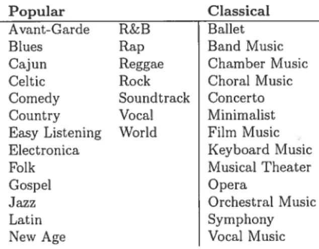
AllMusic1 is a large commercial database offering a range of information about artists, albums and songs, sucli as “Genre”, Style”, “Mood”, ‘Similar Artists” and “Followers”. AilMusic offers a genre for every artist in its comprehensive database. The most popular genre by far is Rock, with about haif of popular artists; other popular genres include Blues, Jazz, and Easy Lis tening. Classical music is not a genre in AilMusic. Instead, classical music is divided among 13 genres such as Ballet, Choral Music, and $ymphony. AllMusic’s full genre taxonomy is listed in table 3.2.
Popular Classical
Avant-Garde RcB Ballet
Blues Rap Band Music
Cajun Reggae Chamber Music
Celtic Rock Choral Music
Comedv Soundtrack Concerto
Country Vocal Ivlinimalist
Easy Listening \Vorld film Music
Electronica Keyboard Music
Folk Musical Theater
Gospel Opera
Jazz Orchestral Music
Latin Symphony
New Age Vocal Music
Table 3.2. AliMusic offers a two-level hierarchy for genre. The first level distinguises popular music from classical, the second level in each branch s given in the columns of the table.
In recognition of the fact that genres are not as precise as many listeners would like, AllMusic lias introduced a number of narrower descriptors: sub-genre categories called ‘Style” and extra-genre descriptors called “Mood”. While only one extra-genre per entry is allowed, multiple Style and Mood labels are often applied to a single artist, and they are not arranged in any hierarchy.
There are three factors that make AIlMusic flot directly usable as a dataset for music classi fication. The first is that AllMusic is exclusively a source of meta-information, it lias no audio component. The second is that AllIViusic is prohibitively expensive to licence and difficult to access automatically via the website. The third is that AllMusic is an evolving taxonomy; the Genre tags are relatively persistent (though their number vas recently raised), but the Mood and
Style descriptors are in more rapid flux. In addition. it is important to remember that AHMusic is foremost a commercial enterprise. flot a music classification project for research.
3.3
USPOP
USPOP2 is a database of full-length songs, together with their AliMusic meta-information. In contrast to the Tzanetakis database, it is flot available as audio—Dan Ellis distributes aIl the music content of the database as pre-computed Mel-scale frequency Cepstral Coefficients (described later in section 4.1.3).
The songs in USPOP were selected to represent popular music. The database is centred around 400 popular artists, as determined by a trawi of the OpenNap peer-to-peer network, circa 2001. One or more albums xvas purchased for each popular artist, and the tracks on those albums make up the music component of the USPOP database. The labels were determined by querying AllMusic.com for each one of the artists (circa 2001). Further details are available at the USPOP website.
It is possible to atternpt several learning tasks using the USPOP database. Each song is associated tvith a single genre and a single artist. Wliile prediction of the Style, Mood, and Sirnilar Artists would be interesting, to my knowledge this has not been attempted.
Entries Albums Artists Styles Genres
USPOP 8764 706 400 251 10
Table 3.3. Summary statistics ofthe USPOP database.
3.4
MIREX 2005
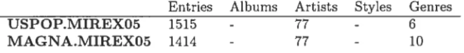
MIREX (Music Information Retrieval Evaluation eXchange) is an annual series of contests, start ing in 2005, whose main goal is to present and compare state-of-the-art algorithms from the music information retrieval community.4 It is organized in parallel with the ISMIR conference (cg. Crawford and Sandler [2005]). The contest encourages many aspects of music information retrieval, embracing both symbolic and signal audio. The most popular contest was the genre competition (with 13 successful participants) that tvas a pair of straightforward multiclass clas sification tasks. The two datasets used to evaluate the submissions were based on Magnatune5, and USPOP6. Both databases contained mp3 files of commercially produced full-length songs. The Magnatune database had a hierarchical genre taxonomy with 10 classes at the most detailed
2www.ee. columbia.edu/dpwe/research/musicsim/uspop2002.html
3OpenNap is an open-source server for thenapster apeer-to-peer file-sharing protocol.
4For example, MIREX 2005 was organized prirnarily via a wiki at http://www.music-ir.org/mirex2005. 5v1agnatune is a record label that licences music under the creative common licence. http://uww.magnatune.com 6www.ee. columbïa. odu/dpwe/research/musicsim/uspop2002.litai
level (ambient, blues, ctassicat, etectronic, ethnic, folk, jazz, new age, punk, rock), whereas US POP.MIREXO5 was a simpler version cf USPOP with 6genres (country, etectronic anti dance, new age, rap anti hip hop, Teggae, Tock). Table 3.4 summarizes the two datasets.
Entries Albums Artists Styles Genres
USPOP.MIREXO5 1515 77 - 6
MAGNA.MIREXO5 1414 77 - 10
Table 3.4. Summary statistics of the data bases used in MIREX 2005.
The overall performance of each entry was calculated by averagÏng the raw classification accu racy on USPOP.MIREXO5 with a hierarchical classification accuracy on MAGNA.MIREXO5.7 Table 3.5 summarizes the contest results.8
Rank Participant Overall Magnatune USPOP
1 Bergstra, Casagrande & Eck[1] 82.34% 75.10% 86.92% 2 Bergstra, Casagrande & Eck[2] 81.77% 74.71% 86.29%
3 Mandel & Ellis 78.81% 67.65% 85.65%
4 West, K. 75.29% 68.43% 78.90%
5 Lidy & Rauber [1] 75.27% 67.65% 79.75%
6 Pampalk, E. 75.14% 66.47% 80.38%
7 Lidy & Rauber [2] 74.78% 67.65% 78.48%
8 Lidy & Rauber [3] 74.58% 67.25% 78.27%
9 Scaringella, N. 73.11% 66.14% 75.74%
10 Ahrendt, P. 71.55% 60.98% 78.48%
11 Burred, J. 62.63% 54.12% 66.03%
12 Soares, V. 60.98% 49.41% 66.67%
13 Tzanetakis, G. 60.72% 55.49% 63.29%
Table 3.5. Summarized resuits for the Genre Recognition contest at MIREX 2005. Square brackets indicate the Index among multiple contest entries.
3.5
FreeDB
FreeDB9 provides music meta-data indexed by a unique compact-disc identifier. Attributes in clude album title, song titles, artist and genre. FreeDB is a volunteer effort; database entries are contributed by users and maintained by volunteers. It is possible for anyone te change entries that are already in the database (in order te correct mistakes), but there is no effort to verify
7More details regarding the evaluation procedure can be found at http://www.music— ir. org/mirex2005/index. php/{Audio_Genre_Classification, Audio_Artist_Identification}.
8More detailed resuits, including class confusion matrices and brief descriptions ofeach algorithm,canbe found at http://www.music—ir.org/evaluation/mirex—results/audio—{genre, artist}/index.litml.
submission before they enter. FreeDB data (and server software) is freely dotvnloadable under the GNU Public Licence10.
FreeDB accepts multiple entries for a given disc, perhaps to accomodate different markup conventions for compilations, re-releases, etc. The consequence is that some artists who have not produced many albums are nevertheiess recognized as the artists of many albums in the database. Also, since records typically are not iabeiled with a genre, freeDB contributors appiy whatever genre labels they wish. Approximately 640 genres in FreeDB have been applied at least 50 times, though typographical errors make it is difficuit to estimate. To summarize, an artist may have many more FreeDB disc entries than bis or her discography would suggest, and those entries may have different genre labels.
The parsing of the FreeDB database for the purpose of building a genre dataset was com piicat.ed because FreeDB is meant to be indexed by a compact-disc table of contents—there is no effort to standardize album titles across releases in different countries, and there is no effort to standardize artist names across albums. To obtain an index of the database by artist, the foilowing aigorithm vas used. Ail artists with more than 10 [databasej records were taken t.o be true artists (there were 20490 of these); ail artists with between 2 and 10 such records were matched against the artists from the first set using a string-matching aigorithm; when a suitable match was found the less-popular artist was merged to the more popular one, otherwise it was discarded; ail artists with just 1 record were discarded; then ail records without a genre label were discarded. Using the remaining records, a histogram over genres tvas built for each remaining artist. This set of histograms indexed by artist is what I wiil refer to as the FreeDB dataset. For convenience, I used a mysterious Levenstein-iike measure created and implemented by Alexandre Lacoste. Aiexandre’s method aligned strings by local edits as weil as block permutations. This made it possible to align string pairs such as Mozart, W.A. and
W.A
Mozart, and recognize the similarity between them.3.5.1
Tags per Track
Figure 3.1 is a histogram of the number of tags per track. Even with log-scahng of the upper axis, there is a convex negative slope that indicates that the vast majority of songs are not labelled very many times. Roughly 100 artists have 40 discs, 500 artists have 20 discs, and 1100 artists have just 5. Few artists have fewer than 5 histogram points because of the parsing and filtering algorithm. On the other end of the graph, many artists have more than 100 database records with genre, and some have as many as 200.
3.5.2
Overali Tag Popularity
Figure 3.2 is a histogram of genre popularity—the total number of applications of each genre. This figure is log-scaled in both axes which gives a (roughly) linear downward slope between
‘°The GNU Public Licence guarantees freedom to use, modify and redistribute intellectual property. For more information, refer te www.gnu.org.
Q Q Q Q n Q Q
Histogram oftags per track 10000 1000 100 10 1 I I I I
E
1-listogram of tag frequencies
0 20 40 60 80 100 120 140 160 180 200
number of tag applications (for a track)
Figure 3.1. On the bottom axis, the ticks indicate the number of total labels (including repetitions) applied to an artist from FreeDB. On the upper axis, the ticks indicate how many artists had a given number of discs.
100
10
1
number of tag applications
Figure 3.2. On the bottom axis, the ticks indicate the logarithm of the popularity of a genre over the entire FreeDB dataset. On the upper axis, the numbers indicate how many genres have a given (Iog) popularity. Note that log-scaling has been appliedto both axes.
Histogram of first-tag importance 1000 100 Q o z 10 1
Figure 3.3. On the bottom axis, the ticks indicate the logarithm of the popularity of a genre over the entire FreeDB dataset. On the upper axis, the numbers indicate how many genres have a given (log) popularity. Note that Iog-scaling has been applied to both axes.
popularity 20 and 100. Most genres have been applied less than 50 times, though rock has been applied almost 100,000 times. This distribution is extremely sharp: there are just 8 genres that have been applied more than 10,000 times, 69 genres with popularity between 1000 and 10,000, about 120 genres with popularity between 100 and 1000, and 424 genres with popularity between 10 and 100
3.5.3
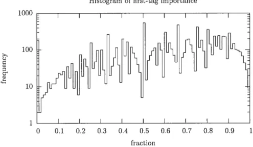
First-Tag Importance
Figure 3.3 is a histogram (over each track) of the fraction of label applications that went to the most popular label for the track. For example, if a track’s most popular label had 4 applications (or votes), the second-most popular had 3, and another had 1, then the fraction that went to the most popular label would 5e 4/(4 + 3 + 1) = 0.5. In Figure 3.3 there is n slight tendency for the
fractions to be greater than 0.5, but a variety of fractions is common.
It is of particular relevance that these fractions are often small because if they had been large, then we would be able to discard non-leading labels without losing much information. This would have been convenient because there are a number of classification algorithms that would then have been applicable to the problem. Instead, we sec in the histogram that discarding non leading labels could well give us a very bad approximation of the tag distribution. It is not yet possible to be confident in that statement though, because there might be another basis for the space of genre tags that admits good approximations of track distributions using 1-hot vectors.” The search for such alternate representations is left for future work.
0 0.1 0.2 0.3 0.4 0.5 0.6 0.7 0.8 0.9
fraction
3.6
LastFM
Last.frn is an internet radio company that provides custom radio streams.’2 Their primary service is called “scrobbling”. Users permit Last.fm to accumulate information on their listening habits through media-player plugins for WinAmp13, iTunes’4, XMMS’5, etc, and in exchange Last.fm connects users with other users with similar taste, as well as new and interesting artists. With this service, Last.fm ammassed a large community of users with a variety of listening habits. More recently they have expanded their services to allow another mechanisms of exploring music called tags, and they have taken advantage of their large listener community to collect a large number of tags for songs, albums and artists.
The LastFM data set is a set of <track, tag-histogram> pairs that have been tagged by one or more users who specifically chose to tag the track, and not the artist or album. In a version of the dataset provided in confidence to me this summer (July 2006) there were 66,191 pairs. For each song, only the most frequent (up to eight) tags are listed and each tag is given with its absolute frequericy. A total of 30,408 tags occur at least once. This represents a dataset that is structurally similar to FreeDB but that is both cleaner and larger. Unfortunately, since it was
only provided recently it is not the focus of this work.
‘2The Last.fm service is located online at http://www.last.fm.
‘3WinAmp is a popular program for playing mp3’s on a Windows computer. 14iTunes is a popular program for playing mp3’s on an Apple
Genre Classification of Recorded
Audio
In section 2.1, I discussed what music genre is and raised some reasons for why one might want to predict it from audio. This chapter presents both known anci novel ways of doing that, elaborating on experiments presented in Bergstra et al. [2006a].
In that article (Bergstra et al. [2006a]), we presented several algorithms for predicting music genre from audio. The primary method vas to use the ensemble learner ADAB00sT to select from a large set of audio features aggregated over short segments of audio. That method proved to be the most effective one in the genre classification contest at MIREX 2005, ancl the second-best method for recogniing artists. furthermore, that article presented evidence that, for a variety of popular feature choices and classification algorithms, the technique of classifying these aggregated features over short audio segments vas sensitive to the segment-length, which could be both too long and too short.
Although I was hrst author, Bergstra et al. [2006a] (attached as appendix C) was a collabo ration. This chapter is entirely my own work, and follows directions of future work suggested in the article. For instance, the audio segmentation technique proposed in Bergstra et al. 12006a] xvas to partition the audio and classify each segment, which unnecessarily couples two variables. This chapter looks into whether it is the segment length that is important, or their number. This chapter also examines whether if is important that each segment be contiguous, or whether choosing an equivalent amount of audio randomly throughout a song is more effective. In an other direction, Mandel and Ellis [2005b] suggest an alternative technique for summarizing each segment, and this chapter evaluates it against. the feature set that won at MIREX 2005. Third: it has long been my suspicion that a particular popular feature set called the Mel-Frequencv Cep stral Coefficients (MFCC, explained below) is not ideal for subsequent classification by a neural network; this chapter examines two alternative features that I call Mel-scale Phon coefficients and Mel-scale Sone coefficients.
The chapter is organized as follows. Section 4.1 describes several well-known audio features,
including their implementation details. Section 4.2 outiines previous work in song classification algorithms for genre. Section 4.3 describes two principles for song segmentation. Section 4.4 describes the proposed Mel-Scale Phon and IViel-Scale Sone coefficients, both in theory and in implementation. Section 4.5 describes two simple neural network topologies, and the learning algorithm used in section 4.6. Section 4.6 presents the performance of many combinations of feature, segmentation method, and classifier on the Tzanetakis problem (recail 3.1), and section 4.6.5 summarizes the findings.
4.1
Frame-level Features to Represent Music
The classification of recorded music presents several challenges that overwhelm a naive application of a vector classification algorithm. One challenge is that a raw music signal that is long enough to capture a recognizable instrument solo or rhythm has on the order of one hundred thousand dimensions. Another challenge is that classification should be invariant to imperceptible signal transformations such as slight acceleration, or shifting by a small number of samples. Another challenge is that small differences in small magnitudes of spectral components may be hidden in the raw waveform by energy in other frequencies but may be perceptually significant. Yet another challenge is that small overail pitch changes are not significant, but small changes in pitch of frequency components relative to one another are significant; the distinction between these is not evident in the raw waveform.
To overcome these challenges, it is conventional to apply feature-extraction algorithms to the raw audio before classifying it. Feature-extraction methods draw inspiration from a variety of sources: signal processing, physics of sound, psychoacoustics, speech perception, and music the ory. Stili, these features act more like ears than music critics; high-level concepts such as the lyrics, instrumentation, meter, and musical structure are beyond the analytic power of current feature-extraction methods. The features described in this section are simple mathematical trans formations designed to capture some perceptually significant aspect of the sound. While each of these features is imperfect in the sense that imperceptibly different audio signals may yield sig nificantly different feature vectors, still, for several standard learning algorithms, they ease the difficulty of generalizing genre decision boundaries from training examples. These transforms apply to frames, short segments of audio on the order of to of a second. In my impIe mentation, a frame vas defined to be 1024 samples at 22050kHz, corresponding to about 47ms of sound. Thus the Nyquist frequency xvas 11025 and when computing the DFT of each frame (recall 2.2.6) the frequency bands were spaced at 21Hz intervals. In my experiments, frames were used to partition the signal; they did not overlap, and there was no gaps between them.
overlap
4.1.1 FFTC
Many dues to the source or nature of a sound take the form of simple patterns that arise in the magnitude components of the DFT of a signal. For example, some percussive instruments like
cymbals and base drums tend to add energy at specific, sometimes even distinctive, frequencies. Other instruments that produce melodic tones are more difficuit to identify, but tone quality of a melodic instrument is stili related to amplitude patterns in T.
FFTC[k] =
F[k]I
(4.1)TheFFTC feature, defined in equation 4.1 from the signal’s DFT, F, was computed by first using FfTW’ to perform a real-to-complex transform of each 1024-sample frarne of the signal. PFTW does not normalize the transform, so that the absolute magnitude of each spectral compo nent is proportional to the length of the frame used to compute it (as suggested by the definition of the DFT in equation 2.4). I considered this dependence on the framelength undesirable for feature extraction, so I scaled each output magnitude by fraten This scaling factor meant that a full-strength input tone (e.g. a pure tone that attained the maximum recordable amplitude) was assigned intensity 1.0. The output of this transformation vas a matrix in which each row bas 512 complex elements, storing the DFT of each audio frame. The number of rows vas proportionai to the length of the recording.
The absolute value of each complex FFT output e + bi vas computed by the simple formula /a2 +52 Each frame was thus reduced to a real-valued vector of 512 elements. In my exper
iments, I’ll refer to an FFTC feature of 32 dimensions; this was obtained by using the first (lowest-frequency) 32 dimensions and discarding the rest.
4.1.2
RCEPS
Real Cepstral Coefficients (recail 2.2.7) are another popular feature deveioped for speech recogni tion. Perhaps the simplestway to compute them is to use the logarithm of 1 to map energy to loudness. Whïle the iogarithm is a crude estimation of loudness, it is computationally cheap. The requisite computations are expressed by equations 4.2 and 4.3 (culled from the Matlab signal processing toolbox), in which Lrceps represents an intermediate computation, and a smali constant
prevents a logarithm of zero when silence is observed.
Lrccps[k] = log(F[k]I+), (4.2)
RCEPS = dct(Lrceps) (4.3)
In principle, a larger -y makes the response in Lrceps more linear with respect to signal intensity. In practice, classification performance vas stable with -y < but deteriorated when -y was
bigger. For my computations I chose -y=
The logarithm and second DFT were performed on the magnitude DFT vectors themselves, so that after the second DfT, 256 real coefficients remained and I kept them ail.
‘FFTW is a widely-used high-performance library implementing Fast Fourier transforms of real and complex signais in one or multiple dimensions. It is hosted online at http://www.fftw3.org.