Eccentricity dependent deep neural networks: Modeling invariance in human vision

Eccentricity dependent deep neural networks:

Modeling invariance in human vision

The MIT Faculty has made this article openly available.

Please share

how this access benefits you. Your story matters.

Citation

Chen,Francis X. et al. "Eccentricity dependent deep neural

networks: Modeling invariance in human vision." 2017 AAAI

Spring Symposium Series, Science of Intelligence: Computational

Principles of Natural and Artificial Intelligence, March 27-29 2017,

Stanford, California, Association for the Advancement of Artificial

Intelligence, March 2017 © 2017 Association for the Advancement of

Artificial Intelligence

As Published

https://www.aaai.org/ocs/index.php/SSS/SSS17/paper/

viewPaper/15360

Publisher

Association for the Advancement of Artificial Intelligence

Version

Author's final manuscript

Citable link

http://hdl.handle.net/1721.1/112279

Terms of Use

Creative Commons Attribution-Noncommercial-Share Alike

Eccentricity Dependent Deep Neural Networks:

Modeling Invariance in Human Vision

Francis X. Chen, Gemma Roig, Leyla Isik, Xavier Boix and Tomaso Poggio

Istituto Italiano di Tecnologia at Massachusetts Institute of Technology, Cambridge, MA 02139

Abstract

Humans can recognize objects in a way that is invariant to scale, translation, and clutter. We use invariance theory as a conceptual basis, to computationally model this phenomenon. This theory discusses the role of eccentricity in human visual processing, and is a generalization of feedforward convolu-tional neural networks (CNNs). Our model explains some key psychophysical observations relating to invariant perception, while maintaining important similarities with biological neu-ral architectures. To our knowledge, this work is the first to unify explanations of all three types of invariance, all while leveraging the power and neurological grounding of CNNs.

Introduction

Invariance means that when a unfamiliar object undergoes transformations, the primate brain retains the ability to rec-ognize it. Under scaling and shifting of a given object, it is well-known that human vision demonstrates this prop-erty (Riesenhuber and Poggio 1999; Logothetis, Pauls, and Poggio 1995). Additionally, changes in background (some-times termed as visual clutter) do not interfere with recog-nition of e.g. faces, on an intuitive level. Such invariance properties indicate a powerful system of recognition in the brain, displaying high robustness.

Computationally modeling invariant object recognition would both provide scientific understanding of the vi-sual system and facilitate engineering applications. Cur-rently, convolutional neural networks (CNNs) (Krizhevsky, Sutskever, and Hinton 2012; LeCun et al. 1989) are the technological frontrunner for solving this class of prob-lem. CNNs have achieved state-of-the-art accuracy in many object recognition tasks, such as digit classification (Le-Cun et al. 1998) and natural image recognition (Krizhevsky, Sutskever, and Hinton 2012; He et al. 2015). In addition, the CNN primitives of convolution and max-pooling are conceptually similar to simple and complex cells in the brain (Serre, Oliva, and Poggio 2007; Serre et al. 2007; Hubel and Wiesel 1968).

However, CNNs fall short in explaining human percep-tual invariance. First, CNNs typically take input at a sin-gle uniform resolution (LeCun et al. 1998; Krizhevsky,

Copyright c 2017, Association for the Advancement of Artificial

Intelligence (www.aaai.org). All rights reserved.

Sutskever, and Hinton 2012). Biological measurements sug-gest that resolution is not uniform across the human vi-sual field, but rather decays with eccentricity, i.e. distance from the center of focus (Gattass, Gross, and Sandell 1981; Gattass, Sousa, and Gross 1988). Even more importantly, CNNs rely on data augmentation (Krizhevsky, Sutskever, and Hinton 2012) to achieve transformation-invariance. This is akin to explicitly showing an object at many scales and po-sitions, to make sure you can recognize it (this is not some-thing humans typically do). Finally, state-of-the-art CNNs may have over 100 processing layers (He et al. 2015), while the human ventral stream is though to have O(10) (Eber-hardt, Cader, and Serre 2016; Serre, Oliva, and Poggio 2007).

Several models have attempted to explain similar phenomena—for instance, HMAX (Serre et al. 2007) pro-vided a conceptual forerunner for our work and evaluated scale- and translation-invariance. Crowding has been stud-ied with approaches such as population coding (Harrison and Bex 2015; van den Berg, Roerdink, and Cornelissen 2010) and statistics (Balas, Nakano, and Rosenholtz 2009; Freeman and Simoncelli 2011; Nandy and Tjan 2012; Kesh-vari and Rosenholtz 2016).

We present a new computational model to shed light on the key property of invariance in object recognition. We use invariance theory properties and rely on CNNs (Anselmi et al. 2016), while maintaining close and explicit ties with the underlying biology (Poggio, Mutch, and Isik 2014). We focus on modeling the brain’s feedforward processing of a single visual glance—this is a reasonable simplification in the study of invariant recognition (Hung et al. 2005; Liu et al. 2009; Serre, Oliva, and Poggio 2007).

The primary advantage of our model is its place at two in-tersections: (1) between the power of CNNs and the require-ment of biological plausibility, and (2) in unifying expla-nations for scale-, translation-, and clutter-invariance. Our model demonstrates invariance properties similar to those in human vision, considering the transformations of scaling, translation, and clutter.

Methods

This section provides an overview of our computational model and methods. For more details we refer the reader to (Chen 2016).

The "Chevron Model"

Poggio et al. Computational role of eccentricity dependent cortical magnification, June 2014.

S

X Implement by modifying image crops.

1 2 3 4 5 6 7

The "Chevron Model"

Poggio et al. Computational role of eccentricity dependent cortical magnification, June 2014.

s

X Implement by modifying image crops.

(a) (b)

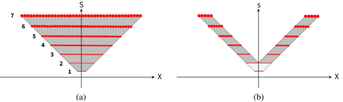
Figure 1: In both figures, the X-axis is eccentricity; the S-axis is scale. (a) Inverted pyramid with sample points: The sample points (small circles) represent visual processing cells. There are 7 ‘scale channels’ numbered from 1 to 7, increasing linearly in diameter. Together, the filters cover the eccentricities and scales in the pyramid, satisfying the scale-invariance requirement. (b) Chevron sampling: Measured receptive fields in macaque monkeys show that some scale channels do not cover all eccen-tricities, suggesting this type of sampling. In this example, the chevron parameter, c, is 2. Note that the light gray central region is an inverted pyramid, similar to Figure 1a.

Conceptual Grounding

A principle of invariance theory is that the brain’s ventral stream derives a transformation-invariant representation of an object from a single view (Anselmi et al. 2016). Fur-thermore, the theory posits a scale-invariance requirement in the brain (Poggio, Mutch, and Isik 2014)—that an object recognizable at some scale and position should be recogniz-able under arbitrary scaling (at any distance, within optical constraints). This requirement is evolutionarily justifiable— scale-invariant recognition allows a person to recognize an object without having to change the intervening distance.

Under the above restrictions, the invariance theory derives that the set of recognizable scales and shifts for a given ob-ject fill an inverted pyramid in the scale-space plane (Fig-ure 1) (Poggio, Mutch, and Isik 2014). Furthermore, the theory suggests that the brain samples the pyramid with the same number of “units” at each scale—this would al-low seamless information transfer between scales (Poggio, Mutch, and Isik 2014). The theory finally relies on pooling over both space and scale as a mechanism for achieving in-variance.

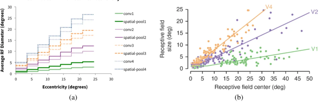
The theory has biological implications—for instance, the hypothesized pooling would increase neural receptive field (RF) sizes from earlier to later areas in the ventral stream. In addition, we would expect average RF sizes to increase with eccentricity. As measured by (Gattass, Gross, and Sandell 1981; Gattass, Sousa, and Gross 1988), shown in Figure 2, both of these are true. However, in Figure 2b we observe that the largest RF sizes seem to be represented only in the periphery, not the fovea. This would be consistent with a

chevron (Poggio, Mutch, and Isik 2014), depicted in

Fig-ure 1b, rather than the inverted pyramid from FigFig-ure 1a. We use this concept of ‘chevron sampling’ in our model.

Model

We build a computational model of the feedforward path of the human system, implementing invariance theory (Poggio, Mutch, and Isik 2014). Our model differs from a conven-tional CNN in a few ways. We detail the characteristics and

architecture of our model below.

Multi-scale input. Our model takes in 7 crops of an in-put image—each is a centered square cutout of the image. The 7 crops are at identical resolution, but different scale, increasing linearly in diameter. Note that the resolution of our model is an order of magnitude less than human vi-sion (Marr, Poggio, and Hildreth 1980; Chen 2016) this trades off fidelity in favor of iteration speed, while main-taining qualitative accuracy.

Chevron sampling. We use our input data to implement ‘chevron sampling’ (see Figure 1b). Let c be the chevron pa-rameter, which characterizes the number of scale channels that are active at any given eccentricity. We constrain the network that at most c scale channels are active at any given eccentricity. In practice, for a given crop, this simply means zeroing out all data from the crop c layers below, effectively replacing the signal from that region with the black back-ground. We use c = 2 for all simulations reported in the Results section.

Convolution and pooling at different scales. Like a conventional CNN, our model uses learned convolutional layers and static max-pooling layers, with ReLU non-linearity (Krizhevsky, Sutskever, and Hinton 2012). How-ever, our model has two unconventional features resulting from its multi-scale nature.

First, convolutional layers are required to share weights across scale channels. Intuitively, this means that it gener-alizes learnings across scales. We guarantee this property during back-propagation by averaging the error derivatives over all scale channels, then using the averages to compute weight adjustments. We always apply the same set of weight adjustments to the convolutional units across different scale channels.

Second, the pooling operation consists of first pooling over space, then over scale, as suggested in (Poggio, Mutch, and Isik 2014). Spatial pooling, as in (Krizhevsky, Sutskever, and Hinton 2012), takes the maximum over unit activations in a spatial neighborhood, operating within a scale channel. For scale pooling, let s be a parameter that indicates the number of adjacent scales to pool. Scale pooling takes the

0 5 10 15 20 25 30 0 5 10 15 20 25 30 Av er ag e RF Diame ter (de gr ees) Eccentricity (degrees)

Our Model - RF Diameter vs. Eccentricity conv1 spatial-pool1 conv2 spatial-pool2 conv3 spatial-pool3 conv4 spatial-pool4

Receptive Fields in the Brain

Freeman et al. Metamers of the ventral stream, September 2011.

Figure from citation.

(a) (b)

Figure 2: (a) Average receptive field (RF) diameter vs. eccentricity in our computational model. (b) Measured RFs of macaque monkey neurons—figure is from (Freeman and Simoncelli 2011).

maximum over corresponding activations in every group of s neighboring scale channels, maintaining the same spatial dimensions. This maximum operation is easy to compute, since scale channels have identical dimensions. After a pool-ing operation over s scales, the number of scale channels is reduced by s − 1.

We define a layer in the model as a set of convolution, spa-tial pooling, and scale pooling operations—one each. Our computational model is hierarchical and has 4 layers, plus one fully-connected operation at the end. These roughly rep-resent V1, V2, V4, IT, and the PFC, given the ventral stream model from (Serre, Oliva, and Poggio 2007). We developed a correspondence between model dimensions and physical dimensions, tuning the parameters to achieve realistic recep-tive field (RF) sizes. Observe the relationship of RF sizes with eccentricity in Figure 2a for our model, compared to physiological measurements depicted in Figure 2b. Notably, macaque RF sizes increase both in higher visual areas and with eccentricity, like our model. In Figure 2a, the sharp ‘cutoffs’ in the plot indicate transitions between different eccentricity regimes. This is a consequence of discretizing the visual field into 7 scale channels. Note that this ignores pooling over scales, to simplify RF characterization. Scale pooling would make RFs irregular and difficult to describe, since they would contain information from multiple scales.

It is not clear from experimental data how scale pooling might be implemented in the human visual cortex. We ex-plore several possibilities with our computational model. We introduce a convention for discussing instances of our model with different scale pooling. We refer to a specific instance with a capital ‘N’ (for ‘network’), followed by four integers. Each integer denotes the number of scale channels outputted by each pooling stage (there are always 7 scale channels ini-tially). For example, consider a model instance that conducts no scale pooling until the final stage, then pools over all scales. We would call this N7771. The results in this paper were generated with N6421 (we call this the ‘incremental’ model), and N1111 (we call this the ‘early’ model).

Input Data and Learning

Our computational model is built to recognize grayscale handwritten digits from the MNIST dataset (LeCun et al. 1998). MNIST is lightweight and computationally efficient, but difficult enough to reasonably evaluate invariance. As shown by (Yamins and DiCarlo 2016), parameters optimized for object recognition using back-propagation can explain a fair amount of variance of the neurons in the monkey’s ven-tral stream. Accordingly, we use back-propagation to learn the parameters of our model on MNIST.

Implementation

Our image pre-processing and data formatting was done in C++, using OpenCV (Bradski 2000). For CNNs, we used the Caffe deep learning library (Jia et al. 2014). Since Caffe does not implement scale channel operations, namely averaged derivatives and pooling over scales, we used custom imple-mentations of these operations, written in NVIDIA CUDA. We performed high-throughput simulation and automation using Python scripts, with the OpenMind High Performance Computing Cluster (McGovern Institute at MIT 2014).

Results

The goal of our simulations is to achieve qualitative similar-ity with well-known psychophysical phenomena. We there-fore design them to parallel human and primate experiments. We focus on psychophysical results that can be reproduced in a ‘feedforward setting.’ This means that techniques such as short presentation times and backward masking are used in an attempt to restrict subjects to one glance (Bouma 1970; Nazir and O’Regan 1990; Furmanski and Engel 2000; Dill and Edelman 2001). This allows for a reasonable compari-son between experiments and simulations. See (Chen 2016) for a more thorough evaluation of this comparison.

The paradigm of our experiments is as follows: (1) train the model to recognize MNIST digits (LeCun et al. 1998) at some set of positions and scales, then (2) test the model’s ability to recognize transformed (scaled, translated, or clut-tered) digits, outside of the training set. This enables eval-uation of learned invariance in the model. Training always

used the MNIST training set, with around 6,000 labeled ex-amples for each digit class. Training digits had a height and

width of 3◦. Networks were tested using the MNIST test set,

with around 1,000 labeled examples per digit class. Each test condition evaluated a single type and level of invariance (e.g.

‘2◦of horizontal shift’), and used all available test digits.

Scale- and Translation-Invariance

We evaluated two instances of our model: N1111, called the ‘early’ model in the plots, and N6421, called the ‘in-cremental’ model. See the Model section under Methods for naming conventions. For comparison, we also tested a low-resolution ‘flat’ CNN, and a high-low-resolution fully-connected network (FCN), both operating at one scale. All networks were trained with the full set of centered MNIST digits.

To test scale-invariance, we maintained the centered po-sition of the digits while scaling by octaves (sizes rounded to the nearest pixel). To test translation-invariance, we

main-tained the 3◦height of the digits while translating. Left and

right shifts were used equally in each condition.

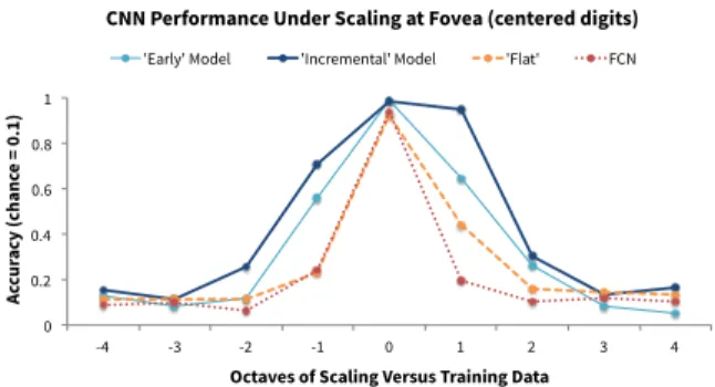
Results are shown in Figures 3 and 4. The exact amount of invariance depends on our choice of threshold. For example, with a 70% accuracy threshold (well above chance), we ob-serve scale-invariance for a 2-octave range, centered at the training height (at best). We observe translation-invariance

for∼0.5◦from the center. Note that our threshold seems less

permissive than (Riesenhuber and Poggio 1999), which de-fined a monkey IT neuron as ‘invariant’ if it activated more for the transformed stimulus than for distractors.

Generally, our results qualitatively agree with experimen-tal data. Synthesizing the results of psychophysical stud-ies (Nazir and O’Regan 1990; ?; Dill and Edelman 2001) and neural decoding studies (Liu et al. 2009; Hung et al. 2005; Logothetis, Pauls, and Poggio 1995; Riesenhuber and Poggio 1999), we would expect to find scale-invariance over two octaves at least. Our model with the ‘incremental’ set-ting (N6421) shows the most scale-invariance—about two octaves centered at the training size. The ‘early’ setting (N1111) performs almost as well as the ‘incremental’ set-ting. The other neural networks perform well on the training scale, but do not generalize to other scales. Note the asym-metry, favoring larger scales. We hypothesize that this re-sults from insufficient acuity.

The translation-invariance of the human visual system is limited to shifts on the order of a few degrees—almost

certainly less than 8◦ (Dill and Edelman 2001; Nazir and

O’Regan 1990; Logothetis, Pauls, and Poggio 1995). Given limited translation-invariance from a single glance in hu-man vision, it is reasonable to conclude that saccades (rapid eye movements) are the mechanism for translation-invariant recognition in practice. The two instances of our model show similar translation invariance, which is generally less than the ‘flat’ CNN and more than the FCN, agreeing with the aforementioned experimental data that shows the limitations of translation-invariance in humans.

Clutter

We focus our simulations on Bouma’s Law (Bouma 1970), referred to as the essential distinguishing characteristic

0 0.2 0.4 0.6 0.8 1 -4 -3 -2 -1 0 1 2 3 4 Ac cur acy (chanc e = 0.1)

Octaves of Scaling Versus Training Data

CNN Performance Under Scaling at Fovea (centered digits)

'Early' Model 'Incremental' Model 'Flat' FCN

Figure 3: CNN performance under scaling at the fovea.

0 0.2 0.4 0.6 0.8 1 0 px 4 px 8 px 12 px 16 px 20 px 24 px 28 px Ac cur acy (chanc e = 0.1)

Shift from Center (1 degree = ~12 px)

CNN Performance Under Translation From Center

'Early' Model 'Incremental' Model 'Flat' FCN

Figure 4: CNN performance under translation from center.

of crowding (Strasburger, Rentschler, and J¨uttner 2011; Pelli, Palomares, and Majaj 2004; Pelli and Tillman 2008). Bouma’s Law states that for recognition accuracy equal to the uncrowded case, i.e. invariant recognition, the spacing between flankers and the target must be at least half of the target eccentricity (see Figure 5). This is often expressed by stating that the critical spacing ratio must be at least b, where b ≈ 0.5 (Whitney and Levi 2011).

We trained our computational model and its variants on all odd digits within the MNIST training set. Training digits were randomly shifted along the horizontal meridian. When testing networks in clutter conditions, we used even dig-its as flankers and odd digdig-its as targets, drawing both from the MNIST test set. Flankers were always identical to one other. We tested several different target eccentricities and

flanker spacings, where each test condition used all∼5,000

odd exemplar targets with a single target eccentricity and flanker spacing. Targets used an even distribution of left and right shifts, and we always placed two flankers radially. In Figure 5, we display the testing set-up used for evaluating crowding effects in our computational model.

Since the neural networks were not trained to identify even digits, they would essentially never report an even digit class. Thus, we could monitor whether the information from the odd digit ‘survived’ crowding enough to allow correct classification. Even digits were used to clutter odd digits only. The psychophysical analogue of this task would be an instruction to ‘Name the odd digit’, with a subject having no prior knowledge of its spatial position.

[1] Pelli et al. The uncrowded window of object recognition, October 2008.

[2] Whitney et al. Visual crowding: A fundamental limit on conscious perception and object recognition, April 2011.

When we try to recognize a particular object, crowding is when nearby objects interfere.

1

2 2

Crowding (usually) follows Bouma's Law—for recognition,

flanker spacing must be at least half of target ecc [1] [2] [3]

[3] Herzog et al. Crowding, grouping, and object recognition: A matter of appearance, 2015.

target eccentricity

flanker spacing

Figure 5: Explaining Bouma’s Law of Crowding. The cross marks a subject’s fixation point. The ‘1’ is the target, and each ‘2’ is a flanker. For recognition accuracy equal to the uncrowded case, flanker spacing (the length of each red ar-row) must be at least half of target eccentricity.

0 0.2 0.4 0.6 0.8 1 0° 2° 4° 6° 8° Ac cur acy (chanc e = 0.2) Flanker Spacing

'Early' Model, Performance Under Clutter

1° target ecc 3° target ecc 5° target ecc 7° target ecc 9° target ecc

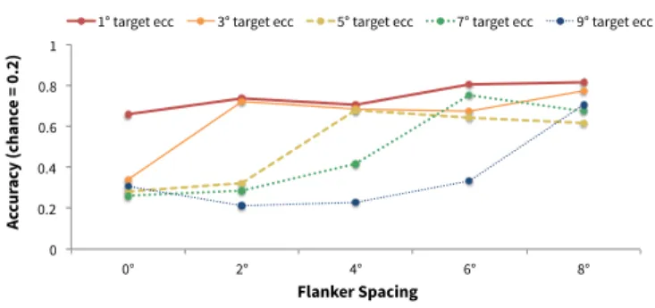
Figure 6: ‘Early’ model performance under clutter. Each line has constant target eccentricity. We observe the same quasi-logistic trend as is shown in (Whitney and Levi 2011).

0 0.2 0.4 0.6 0.8 1 0 0.2 0.4 0.6 0.8 1 Ac cur acy with 2 T ang ential Flank er s (chanc e = 0.2)

Accuracy with 2 Radial Flankers (chance = 0.2) 'Early' Model Accuracy Under Clutter,

Radial vs. Tangential Flankers

Figure 7: Radial-tangential anisotropy in our model.

We focus on the ‘early’ model comparing our results with the description of Bouma’s Law in (Whitney and Levi 2011). We do not report results for the other models as they per-form poorly compared to the ‘early’ model in this task. In Figure 6, we plot our simulation results using their con-vention, which evaluates performance when target eccen-tricity is held constant and changing the target-flanker sep-aration. We find a similar trend compared to human sub-ject data, where recognition accuracy increases dramatically near b ≈ 0.5. However, accuracies ‘saturate’ near 0.7. This results might be from the lack of a selection mechanism in the model (there is no way to tell it to ‘report the middle digit’).

In addition, we find that our model displays radial-tangential anisotropy in crowding—radial flankers crowd

more than tangential ones (Whitney and Levi 2011). As of (Nandy and Tjan 2012), biologically explaining this phe-nomenon has been an open problem. We tested this using a variation on our Bouma’s Law procedure, where training digits used random horizontal and vertical shifts, and test sets evaluated radial and tangential flanking separately. Out of 25 test conditions with different target eccentricities and flanker spacings, 24 displayed the correct anisotropy in our model (see Figure 7). This leads to a principled biological explanation—scale pooling (the distinguishing characteris-tic of the model) operates radially, which causes radial sig-nals to interfere over longer ranges than tangential sigsig-nals. Unlike (Nandy and Tjan 2012), this explanation does not rely on saccades and applies to the feedforward case.

Discussion and Conclusions

We have presented a new computational model of the feed-forward ventral stream, implementing the invariance the-ory and the eccentricity dependency of neural receptive fields (Poggio, Mutch, and Isik 2014). This model achieves several notable parallels with human performance in object recognition, including several aspects of invariance to scale, translation, and clutter. In addition, it uses biologically plau-sible computational operations (Serre et al. 2007) and RF sizes (see Figure 2).

By considering two different methods of pooling over scale, both using the same fundamental CNN architec-ture, we are able to explain some key properties of the human visual system. Both the ‘incremental’ and ‘early models explain scale- and translation-invariance properties, while the ‘early’ model also explains Bouma’s Law and radial-tangential anisotropy. The last achievement could be significant—previous literature has not produced a widely-accepted explanation of radial-tangential anisotropy (Nandy and Tjan 2012; Whitney and Levi 2011). Furthermore, we obtained our results without needing a rigorous data-fitting or optimization approach to parameterize our model.

Of course, much work remains to be done. First, there are two notable weaknesses in our model: (1) low acuity relative to human vision, and (2) the lack of a ‘selection mechanism’ for target-flanker simulations. Though the first may be rela-tively easy to solve, the second raises more questions about how the brain might solve this problem.

In the longer term, it would be even more informative to explore natural image data, e.g. ImageNet (Russakovsky et al. 2015). In addition, further work could be conducted in developing a correspondence between our model and real psychophysical experiments. Finally and most promisingly, it would be interesting to explore approaches for combining information from multiple glimpses, as in (Ba, Mnih, and Kavukcuoglu 2015). Such work could build upon our find-ings and expose even deeper understandfind-ings of the human visual system.

Acknowledgments

This work was supported by the Center for Brains, Minds and Machines (CBMM), funded by NSF STC award CCF - 1231216. Thanks to Andrea Tacchetti, Brando Miranda,

Charlie Frogner, Ethan Meyers, Gadi Geiger, Georgios Evangelopoulos, Jim Mutch, Max Nickel, and Stephen Voinea, for informative discussions. Thanks also to Thomas Serre for helpful suggestions.

References

Anselmi, F.; Leibo, J. Z.; Rosasco, L.; Mutch, J.; Tacchetti, A.; and Poggio, T. 2016. Unsupervised learning of invariant representa-tions. Theoretical Computer Science 633:112–121.

Ba, J. L.; Mnih, V.; and Kavukcuoglu, K. 2015. Multiple ob-ject recognition with visual attention. International Conference on Learning Representations.

Balas, B.; Nakano, L.; and Rosenholtz, R. 2009. A summary-statistic representation in peripheral vision explains crowding.

Journal of Vision9(12):13.1–13.18.

Bouma, H. 1970. Interaction effects in parafoveal letter recogni-tion. Nature 226:177–178.

Bradski, G. 2000. OpenCV library. Dr. Dobb’s Journal of Software Tools.

Chen, F. 2016. Modeling human vision using feedforward neural networks. Master’s thesis, Massachusetts Institute of Technology. Dill, M., and Edelman, S. 2001. Imperfect invariance to object translation in the discrimination of complex shapes. Perception 30:707–724.

Eberhardt, S.; Cader, J.; and Serre, T. 2016. How deep is the feature analysis underlying rapid visual categorization? arXiv:1606.01167 [cs.CV].

Freeman, J., and Simoncelli, E. P. 2011. Metamers of the ventral stream. Nature Neuroscience 14(9):1195–1201.

Furmanski, C. S., and Engel, S. A. 2000. Perceptual learning in object recognition: Object specificity and size invariance. Vision

Research40:473–484.

Gattass, R.; Gross, C.; and Sandell, J. 1981. Visual topography of V2 in the macaque. The Journal of Comparative Neurology 201:519–539.

Gattass, R.; Sousa, A.; and Gross, C. 1988. Visuotopic organi-zation and extent of V3 and V4 of the macaque. The Journal of

Neuroscience8(6):1831–1845.

Harrison, W. J., and Bex, P. J. 2015. A unifying model of orienta-tion crowding in peripheral vision. Current Biology 25:3213–3219. He, K.; Zhang, X.; Ren, S.; and Sun, J. 2015. Deep residual learn-ing for image recognition. arXiv:1512.03385 [cs.CV].

Hubel, D., and Wiesel, T. 1968. Receptive fields and

func-tional architecture of monkey striate cortex. Journal of Physiology 195:215–243.

Hung, C. P.; Kreiman, G.; Poggio, T.; and DiCarlo, J. J. 2005. Fast readout of object identity from macaque inferior temporal cortex.

Science310:863–866.

Jia, Y.; Shelhamer, E.; Donahue, J.; Karayev, S.; Long, J.; Girshick, R.; Guadarrama, S.; and Darrell, T. 2014. Caffe: Convolutional architecture for fast feature embedding. arXiv:1408.5093 [cs.CV]. Keshvari, S., and Rosenholtz, R. 2016. Pooling of continuous features provides a unifying account of crowding. Journal of Vision 16(3):39.1–39.15.

Krizhevsky, A.; Sutskever, I.; and Hinton, G. E. 2012. ImageNet classification with deep convolutional neural networks. Advances in Neural Information Processing Systems.

LeCun, Y.; Boser, B.; Denker, J.; Henderson, D.; Howard, R.; Hub-bard, W.; and Jackel, L. 1989. Handwritten digit recognition with

a back-propagation network. Advances in Neural Information Pro-cessing Systems.

LeCun, Y.; Bottou, L.; Bengio, Y.; and Haffner, P. 1998. Gradient-based learning applied to document recognition. Proceedings of the IEEE.

Liu, H.; Agam, Y.; Madsen, J. R.; and Kreiman, G. 2009. Timing, timing, timing: Fast decoding of object information from intracra-nial field potentials in human visual cortex. Neuron 62:281–290. Logothetis, N. K.; Pauls, J.; and Poggio, T. 1995. Shape represen-tation in the inferior temporal cortex of monkeys. Current Biology 5(5):552–563.

Marr, D.; Poggio, T.; and Hildreth, E. 1980. Smallest channel in early human vision. Journal of the Optical Society of America 70(7):868–870.

McGovern Institute at MIT. 2014. OpenMind: High performance computing cluster.

Nandy, A. S., and Tjan, B. S. 2012. Saccade-confounded image statistics explain visual crowding. Nature Neuroscience 15(3):463– 469.

Nazir, T. A., and O’Regan, J. K. 1990. Some results on translation invariance in the human visual system. Spatial Vision 5(2):81–100. Pelli, D. G., and Tillman, K. A. 2008. The uncrowded window of object recognition. Nature Neuroscience 11(10):1129–1135. Pelli, D. G.; Palomares, M.; and Majaj, N. J. 2004. Crowding is unlike ordinary masking: Distinguishing feature integration from detection. Journal of Vision 4:1136–1169.

Poggio, T.; Mutch, J.; and Isik, L. 2014. Computational role of eccentricity dependent cortical magnification. Memo 17, Center for Brains, Minds and Machines.

Riesenhuber, M., and Poggio, T. 1999. Hierarchical models of ob-ject recognition in cortex. Nature Neuroscience 2(11):1019–1025. Russakovsky, O.; Deng, J.; Su, H.; Krause, J.; Satheesh, S.; Ma, S.; Huang, Z.; Karpathy, A.; Khosla, A.; Bernstein, M.; Berg, A. C.; and Fei-Fei, L. 2015. ImageNet large scale visual recognition challenge. International Journal of Computer Vision 115(3):211– 252.

Serre, T.; Wolf, L.; Bileschi, S.; Riesenhuber, M.; and Poggio, T.

2007. Robust object recognition with cortex-like mechanisms.

IEEE Transactions on Pattern Analysis and Machine Intelligence 29(3):411–426.

Serre, T.; Oliva, A.; and Poggio, T. 2007. A feedforward architec-ture accounts for rapid categorization. Proceedings of the National

Academy of Sciences (PNAS)104(15):6424–6429.

Strasburger, H.; Rentschler, I.; and J¨uttner, M. 2011.

Periph-eral vision and pattern recognition: A review. Journal of Vision 11(5):13.1–13.82.

van den Berg, R.; Roerdink, J. B.; and Cornelissen, F. W. 2010. A neurophysiologically plausible population code model for feature integration explains visual crowding. PLoS Computational Biology 6(1).

Whitney, D., and Levi, D. M. 2011. Visual crowding: A fundamen-tal limit on conscious perception and object recognition. Trends in

Cognitive Sciences15(4):160–168.

Yamins, D. L., and DiCarlo, J. J. 2016. Using goal-driven deep learning models to understand sensory cortex. Nature neuroscience 19(3):356–365.