Dynamics of RC trees with distributed constant-power loads

Dynamics of RC Trees with Distributed Constant-Power

Loads

by

Ben Wing Lup Leong

Submitted to the Department of Electrical Engineering and Computer

Science

in partial fulfillment of the requirements for the degrees of

Bachelor of Science in Electrical Science and Engineering

and

Master of Engineering in Electrical Engineering and Computer Science

at the

MASSACHUSETTS INSTITUTE OF TECHNOLOGY

May 1997

©

Ben Wing Lup Leong, MCMXCVII. All rights reserved.

The author hereby grants to MIT permission to reproduce and distribute

publicly paper and electronic copies of this thesis document in whole or in

part, and to grant others the right to do so.

A uthor...

...

...

Department of Electrical Engineering and Computer Science

May 17, 1997

Certified by ... ...

...

George C. Verghese

Professoof-)·lectrical Engineering

Thiess Supervisor

Accepted by... ....-...-.

...

Arthur C. Smith

Chairman, Department Committee on Graduate Theses

Dynamics of RC Trees with Distributed Constant-Power Loads

by

Ben Wing Lup Leong

Submitted to the Department of Electrical Engineering and Computer Science on May 17, 1997, in partial fulfillment of the

requirements for the degrees of

Bachelor of Science in Electrical Science and Engineering and

Master of Engineering in Electrical Engineering and Computer Science

Abstract

Broadband (fiber optic or coaxial cable) systems are becoming more common as the con-sumer's demand for more bandwidth to the home increases. This thesis presents the results of a study into the dynamic and static stability properties of the networks used to power such systems. An RC tree is used to model the network itself, and a constant-power (P) model is used to represent the loads at each node of the network.

Given an RCP-tree network that satisfies a set of layout constraints, we show that it can be modeled as a gradient system. From this fact, we conclude that the system must end up at one of the possible equilibria of the system. Simple sufficient conditions for the system to end up at a desirable equilibrium are derived from the study of these equilibria. Finally, the application of these results to network and load design is demonstrated, and a proposed approximation model for estimating total current consumption and power dissipation is evaluated.

We show in this thesis that the sufficient stability conditions derived are good guidelines for network design, and that the proposed approximation model is effective in obtaining good estimates.

Thesis Supervisor: George C. Verghese Title: Professor of Electrical Engineering

Acknowledgments

First and foremost, I want to express my heartfelt gratitude towards Professor George C. Verghese, my thesis supervisor. Without his encouragement and guidance, this thesis could never have become reality. George has also been my academic advisor here at MIT since my sophomore year. He strikes me as a patient teacher and a hardworking man who is always in need of sleep. Yet, he makes the effort to find time in his busy schedule to be available to his students. It is impossible for me to thank him enough with a finite number of words. At the same time, I want to thank Vivian Mizuno, George's secretary, for all her help with the administrative trivia that I have had to deal with over the years.

With regard to the technical assistance that I received while working on this thesis, I would like to thank Dr. Joseph Thottuvelil from Lucent Technologies for providing me with valuable information and data on practical broadband power networks, as well as the benchmark model that was eventually used to evaluate the results derived in this thesis. Also, I would like to thank Professor John Wyatt for his pointers and suggestions which were extremely helpful during the initial stages of the work for this thesis.

Among all the people that have made my last four years at MIT memorable, I would first like to acknowledge Tracey Ho, my girlfriend, for her undying love and dedication. I would also like to thank her for encouraging me on during the times when I got depressed over this thesis, and for assisting in the writing and proof-reading of this document.

Pistol has been an integral part of my life over the last four years. I would like to thank Pat Melaragno, my former pistol coach, for teaching me the art of pistol shooting and for

being a wonderful friend and mentor. The road trips that we made together will forever remain my fondest memories of life in MIT.

Without friends, life at MIT would be pretty bleak. I would like to thank all my friends here at MIT - Alice Wang, Chiangkai Er, Danny Yu, Evelyn Huang, Huan Yao, Michael

Sy, Myong-Sin Yi, Steve Lee, Tammy Yap, Tommy Ng, Tseh-Hwan Yong, Weiyang Cheong,

and lots of other wonderful people, for making MIT a most memorable experience.

Finally, I want to thank my parents and family members for being supportive all these years that I have been away from home. I also would like to acknowledge the support that I received from the Public Service Commission of Singapore, which made it possible for me to finance my four years of education here at MIT.

Contents

1.5.2 Non-Ideal Constant-Power Load with Voltage Cutoff ... 25

1.6 Summary of Contributions of this Thesis . ... . . . 26

2 System Modeling and Dynamics: Second-Order System 29 2.1 Preliminary Analysis ... 30

2.2 Gradient System Representation ... .... 32

2.2.1 Gradient System ... 33

2.2.2 Energy Function for Ideal Loads . ... 35

2.2.3 Energy Function for Non-Ideal Loads . ... 36

2.2.4 Application ... ... 38

2.3 Boundary Behavior ... ... 40

2.4 Steady-State Analysis ... 44

2.5 Summary of Results for Second-Order System. . ... . 47

3 System Modeling and Dynamics: Higher-Order Systems 49 7

3.1 Gradient System Representation . . . . 3.2 Characterizing Equilibria . . . .... ... . . . .

3.2.1 _{Types of Equilibria . . . .} 3.2.2 Boundary Conditions . . . . 3.3 Static Equilibria . . . . ... . . . .

3.3.1 Constraint on Cutoff Voltages ...

3.3.2 Characterization of the Hessian . . . . 3.3.3 Guaranteeing Stability for Regular Ladder Network . . . . 3.4 Dynamic Equilibria ...

3.4.1 Boundary Behavior of Modified Gradient System . . . . 3.4.2 Application of Steady-State Analysis to Regular Ladder Network 3.5 Summary of Results for Higher-Order Systems . . . .

4 Computing Equilibria for a Network

4.1 Static Equilibria ... ... ... 4.1.1 Direct Numerical Solution ...

4.1.2 Small-Resistance Approximation . . . . 4.1.3 Approximation Using Aggregated Models . . . . 4.1.4 Iteration and Circuit Simulation . . . . 4.2 Dynamic Equilibria ...

5 Network Design

5.1 Background ...

5.2 Benchmark Model for a Practical Broadband Power Network . 5.3 Stability Conditions ... 5.3.1 Static Equilibria ... 5.3.2 Dynamic Equilibria ... 5.4 Application of Results ... 5.4.1 Guaranteeing Stability ... 87 ... ... 87 . . . . . . 89 ... 90 ... 90 ... 90 . . . . 91 . . . . 91 . 49 51 51 . 52 53 53 54 56 60 60 . 63 . 69 71 71 71 73 80 . 84 85

5.4.2 Estimating Operational Current Load and Power Dissipation . . . 5.5 Varying the Cutoff Voltage ...

5.6 Sum m ary ... .... ... .... ... . ... .... .. . . .

6 Conclusion

6.1 Future Work . . . .

A Detailed Boundary Analysis for Second-Order System A.1 Boundary: v = ... A.2 Boundary: v2 = V ... B Determinant Calculations B.1 Second-Order System ... B.2 Third-Order System ... B.3 Higher-Order Generalization . . . . B.4 Computing the Inequality Coefficient . . . . B.5 Approximation for Sufficient Condition Coefficient . . . .

C Numerical Solutions with Maple V

C.1 Second-Order System...

C.2 Third-Order Ladder...

D Small-Resistance Approximation D.1 Third-Order System ... D.2 Generalization...

E Evaluation of Aggregated Models E. 1 The Models ...

E. 1.1 Series Model ...

E. 1.2 Parallel Model ....

E.2 Evaluation of the Series Model

... ... ... ... ...

...

...

9

E.2.1 Approximation in Second-order System . ... 134

E.2.2 Approximation in Third-order System . ... 135

E.3 Evaluation of the Parallel Model ... .... 138

E.3.1 Approximation in Second-order System . ... 139

List of Figures

1-1 Diagram showing an example HFC powering network. . ... 18

1-2 Diagram showing an example FTTC powering network. ... 19

1-3 Current versus voltage characteristic for ideal constant-power load ... 21

1-4 Typical input current versus voltage characteristic for constant-power load with voltage cutoff V~ ... 22

1-5 Modeling of system dynamics. ... 23

1-6 Equivalent second-order model. . ... .... 23

1-7 Circuit diagram for first-order system. ... . 24

1-8 Dynamic behavior for first-order system. . ... 25

1-9 Dynamic behavior for first-order system with cutoff V. ... . 26

1-10 Dynamic behavior for situation with no real roots. ... . . 26

2-1 Circuit diagram for second-order system. . ... . . 30

2-2 Plot of il = 0 and b2 = 0 loci for second-order system ... . . . . .. 32

2-3 Vector fields for second-order system. ... . .. 33

2-4 Example plot ofE(v, v2). ... 37

2-5 Example plot of E(vl, v2) (different angle). . ... 38

2-6 Phase-plane portrait for second-order system with cutoff. ... 42

2-7 Regular second-order system ... 44

3-1 An nth-order tree network with branching. . ... 50

3-2 An example of current flow ... 54

3-4 Converging field lines at the non-differentiable boundary.

3-5 Sliding effect along non-differentiable boundary. . ... 62

3-6 Third-order system . ... ... .. 64

3-7 Example nth-order system. . ... ... 66

4-1 Second-order system. . ... ... 73

4-2 Third-order system ... . . . . ... . . . 76

4-3 Error convergence ... 80

4-4 Second-order series configuration. ... ... . . 83

4-5 Second-order parallel configuration. ... . . . 83

4-6 Aggregated model. ... 84

5-1 Schematic for practical series broadband network layout. ... 89

5-2 Practical model for broadband network. . ... 89

5-3 First-order aggregated-model approximation. . ... 95

A-1 Diagram of boundary vl = V ...

105

A-2 Diagram of boundary v

= V. ...

107

B-1 Plot of f(n) against n. ...

116

B-2 Error for approximation of f(n) ... 116

C-1 Graphical method for obtaining solutions to a second-order system. .... 120

C-2 Example field plot for second-order system (ideal loads). ... 121

C-3 Example field plot for second-order system (non-ideal loads)... . . . 122

D-1 Third-order system ... 125

D-2 Circuit diagram for first-order system. ... . . . 128

D-3 A third-order example with branching. ... . . . 129

D-4 Example loop with equivalent circuit. ... . . . 129

E-1 E-2 E-3 E-4 E-5 E-6 E-7 E-8 E-9 E-10 E-11 E-12

Second-order series configuration with aggregated model. ... Plot of current vs time for second-order series configuration. ... Plot of current vs time for series aggregated model (second-order). Example third-order series configuration . . . . .

Aggregated models for third-order series configuration. ... Plot of vl vs t for third-order series configuration. ... Plot of v' vs t for series approximation (third-order). ... Second-order parallel configuration with aggregated model . ...

Example third-order parallel configuration . . . . .

Aggregated model for third-order parallel configuration . . . . .

Plot of vl vs t for third-order parallel configuration. ... Plot of v' vs t for parallel approximation (third-order). ...

S. . . .134 S. . . .136 S. . . .137 S. . . .137 S. . . . 138 S. . . . 139 . . . 140 S. . . . 141 S. . . . 141 S. . . . 141 S. . . .142 S. . . .143

List of Tables

3.1 Cutoff Voltage Coefficients for Regular Ladder Networks (Static Equilibria)

3.2 Cutoff Voltage Coefficients for Regular Ladder Networks (Dynamic

Equi-libria) . . . . 4.1 Table of Approximation Results for a Second-Order System ...

4.2 Demonstration of Convergence ...

5.1 Cutoff Voltage Coefficients for Broadband Power Network Model (Static Equilibria) . . . . 5.2 Cutoff Voltage Coefficients for Broadband Power Network

namic Equilibria) ...

5.3 Steady-State Voltages and Currents for 9th-order System .. 5.4 Steady-State Voltages and Currents for 10th-order System

5.5 Steady-State Currents and Aggregated-Model Estimates ...

5.6 Minimization of Coefficient g (n). . ...

Model

(Dy-B.1 Errors for Approximation of f(n) ...

E.1 Table of Results for Series Configuration (Second-Order) . E.2 Table of Results for Series Configuration (Third-Order) .. E.3 Table of Results for Parallel Configuration (Second-Order) E.4 Table of Results for Parallel Configuration (Third-Order)

. . . .115

S . . . . .135

S . . . 138

S . . . 139

Chapter 1

Introduction

1.1 Background

Broadband (fiber optic or coaxial cable) systems are becoming more common as the con-sumer's demand for more bandwidth to the home increases. The analysis of broadband networks to obtain accurate cost and performance predictions becomes correspondingly important. This thesis focuses on issues of "broadband power," namely those associated with delivering power to broadband networks, and is concerned mainly with the dynamic and static stability properties of such networks. Very little analytical work has been done so far on this in the literature. In this thesis, an RC-tree is used to model the network itself, and a constant-power (P) model is used to represent the load at each node of the network once the load voltage exceeds a certain critical level.

There are two broadband architectures that are currently being implemented [1]: the Hybrid Fiber Coax (HFC) architecture and the Fiber-To-The-Curb (FTTC) architecture. For the HFC architecture, fiber serves a group of many homes and coaxial cable is used to provide both power and RF to the homes via amplifiers and Network Interface Units (NIUs) at each home. For the FTTC architecture, Optical Network Units (ONUs) are powered by a network that is independent of the data network. Topologically, HFC networks are

either bus-like or tree-like networks, while FTTC networks are either bus-like or point-to-point networks. Since a bus-type network requires a shorter total length of fiber than a corresponding point-to-point network, the former is generally a more attractive approach

for a FTTC network.

Examples of HFC and FTTC networks discussed in [1] are reproduced in Figures 1-1 and 1-2. In these examples, the cables have the following resistances per unit length: Type

860 - 0.724 mQ/foot, Type 715 - 0.997 mQ/foot, Type 750 - 0.75 mQ/foot and Type 540

- 1.61 mQ/foot. The power ratings for typical NIUs and ONUs are 7 W and 100 W respec-tively; typical capacitances associated with these loads are about 10 to 20 HF/watt, i.e. a 100 W load might have a capacitance of 1000 MF to 2000 pF. Current safety regulations prohibit the power source voltage from exceeding 150 V and the typical power source is rated at 90 V, though this value can fall to about 75 V at the end of the battery life for these sources.

- Power Source

( Optical Network Unit (ONU)

Figure 1-2: Diagram showing an example FTTC powering network.

1.2 Interesting Problems

Since there is presently very little analytical knowledge of the properties of broadband networks, there is a whole spectrum of questions that are of interest to a network designer. This section outlines a variety of relevant problems of interest.

At a very basic level, it is straightforward to obtain an analytical solution for a first-order system, but with higher-order systems there is too much nonlinearity to obtain analytical so-lutions. As a result, the equilibria for higher-order networks are only obtained numerically. The questions of interest include: how many equilibria are there for arbitrary higher-order network topologies? How many of these are stable operating points? We will show later in Section 3.2.2 that for any arbitrary RCP-tree network at least one stable equilibrium is guaranteed to exist.

Also of interest is the dynamic behavior of a network. Basically, given the initial con-dition of a network, it would be useful if the dynamical evolution of the system can be modeled accurately. This would allow for the prediction of the eventual steady state of the system, if such a state exists. It is known that the operating point of a network depends critically on the cutoff voltage of the constant-power load. Empirical observations from

low-order network topologies suggest that for a reasonable network with real equilibria, there exists at least one stable and desirable equilibrium and one undesirable equilibrium. It is clear that if the cutoff voltage is chosen carefully, all the undesirable equilibria can be eliminated and the network can be guaranteed to reach a desired stable equilibrium, but it is unclear if there is a systematic way to arrive at a good choice, or even what constitutes a good choice. Do we want the system to settle at the desired operating point in the shortest amount of time from any initial state? Do we just want a guarantee that a desired operating point is reached at steady state? For the purposes of this thesis, we focus on guaranteeing that the system will end up at a desired operating point, starting from any initial conditions. In this thesis, a network will be termed stable if it will end up at a desired steady-state

equilibrium starting from any initial conditions.

For a first-order system, it is obvious from some elementary analysis (see Section 1.5) that L is the optimal cutoff to guarantee stability, where V is the voltage of the power source. With this cutoff voltage, the system is guaranteed to reach the desirable operating point from any initial state. The appropriate choice of cutoff for higher-order systems is not obvious. In fact, it is unclear whether there always exists a cutoff that guarantees stability for an arbitrary network topology. At present, the recommended cutoff for constant-power nodes in existing broadband power networks is E, but no one can say anything more than "it seems to work." The analytical justification that this is a good choice under certain conditions is a major result for this thesis.

As mentioned in Section 1.1 above, bus-like networks are common in both HFC and FTTC architectures. Regular ladder networks, where all resistances, all capacitances and all loads are identical, are of particular interest in network design, because many practical networks are well modeled this way, and also because the results for this case form a bench-mark and guide to the behavior of more general networks. This thesis devotes particular attention to regular ladder networks.

1.3 Constant-Power Load

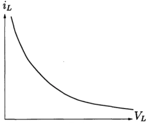
The loads in a broadband power network typically comprise high-efficiency regulated swit-ching power supplies that maintain essentially constant voltage across the components that they feed. Such loads are therefore well-modeled as power loads. A constant-power (P) load is a component that dissipates a constant amount of constant-power independent of the voltage across it. Ideally, the voltage-current characteristic would look like the curve shown in Figure 1-3.

_ VT.

Figure 1-3: Current versus voltage characteristic for ideal constant-power load. In practice, however, it is impossible and impractical to have an ideal constant-power load because there is an upper limit on the current that can be supplied. Limits on voltage are naturally imposed by the fact that the source voltage is fixed at V. A more realistic model of a practical constant-power load would be one with a low-voltage cutoff, Vc, such that the load turns off and draws close to zero current once the voltage across it drops below the cutoff voltage, i.e.

P', 0 < V*

<I 0

iL = VL

0, vL < VC*

A typical input current versus voltage characteristic for such a load is shown in Fig-ure 1-4. Henceforth, a load with the characteristic in FigFig-ure 1-3 will be referred to as a "ideal constant-power load" while the load in Figure 1-4 will be referred to as a "non-ideal constant-power load" or simply as a "constant-power load."

VL

Figure 1-4: Typical input current versus voltage characteristic for constant-power load with voltage cutoff V,.

In practice, some hysteresis is designed into a constant-power load, i.e. the voltage at which the load turns "on" and draws current is set a little higher than the voltage at which it shuts off once turned "on." In this thesis, we will assume that loads behave ideally, and that the cutoff voltage is the same when the system moves in either direction. Also, we assume

that when VL = V, it is possible for the load at operate at any current between 0 and imax

(e.g. by switching between the "on" and "off" states with the appropriate duty cycle). We will refer to this region of operation when the current-voltage characteristic is vertical with

VL = V, as the metastable region. Similarly, we will refer to the region when the load is

"off' as the cutoff region. When the load is operating past the metastable region, we will refer to the load as being on.

1.4 Circuit Models

In the network topologies to be analyzed, the constant-power load elements are modeled as described in Section 1.3, with current-voltage characteristics as shown in Figure 1-4. In addition, the dynamics of the systems are modeled by introducing a suitable capacitor across each constant-power load. Figure 1-5 shows a typical second-order example. The main network topologies studied in this thesis are RCP trees, with particular emphasis on

ladder networks since they effectively model bus-like networks common in both HFC and FTTC architectures.

Figure 1-5: Modeling of system dynamics.

In [1], networks are modeled with another resistor along the return path instead of having all the constant-power loads attached to a common ground. An example of a second-order system modeled in this way is shown in Figure 1-6. A closer look, however, reveals that the two circuit models in Figures 1-5 and 1-6 are in fact entirely equivalent in terms of dynamic behavior and steady-state current flow and power dissipation when R1 = Ri,a +

Rl,b and R2 = R2,a + R2,b. The model in Figure 1-5 is simpler, however, since there are

fewer resistors, so it is the model of choice for this thesis.

P2

Figure 1-6: Equivalent second-order model.

1.5 First-Order System

Before diving into the detailed analysis of general RCP networks, we present the analysis of the simplest possible RCP configuration - a first-order RCP system. This analysis will provide some preliminary insight into the dynamics of RCP networks. We begin with the simpler ideal constant-power model and then later extend the results to the non-ideal model.

1.5.1 Basic System

We analyze the dynamics of a simple network with one constant-power load by modeling the load as a capacitor in parallel with an ideal constant-power load of the sort described in Section 1.3; it draws a constant amount of power regardless of the voltage across it. Figure 1-7 shows this first-order model.

R

V P

Figure 1-7: Circuit diagram for first-order system.

By Kirchhoff's Current Law,

dv V - v P C-- = - - v _(1.1) dt R v 1 = ( v₂ - Vv + PR) _(1.2)

Rv

Solving for the roots of the quadratic expression, we obtain V JVV2 - 4PR

v = - =. (1.3)

2 2

Assuming V2 > 4PR, there are two real roots. Defining v+ = + 4PR and v =

v - ,PR (1.2) can be written as

dv (v - v+)(v - v_)

(1.4)

dt CRv

From (1.4), we deduce that the sign of the derivative is negative when 0 < v < v_, pos-itive when v_ < v < v+, and finally negative when v+ < v < V. Figure 1-8 is a graphical representation of this result. The interpretation of this result is straightforward: v_ is an

unstable equilibrium point, while v+ is a stable equilibrium point. If the system starts at an initial condition such that v_ < v < V, the system will come to rest at v+, while an initial condition where 0 < v < v_ will result in v falling to 0.

V

0 .v_ - v+ V

Figure 1-8: Dynamic behavior for first-order system.

1.5.2 Non-Ideal Constant-Power Load with Voltage Cutoff

From the analysis of the system dynamics in the previous subsection, it is that apparent that there is no obvious way for the system to make a transition from a zero initial condition to the desired stable operating equilibrium. If the system were to start off at the origin, it would stay stuck at the origin. We can get around this problem by replacing the ideal load with a non-ideal load that has a voltage cutoff, V, chosen higher than v_.

With this new load, the circuit is equivalent when v < V, to a simple DC voltage source charging a capacitative load. The behavior of the system when v > V, is the same as that described in the previous subsection. With this, we effectively remove the lower equilibrium and the system ends up with a single stable static equilibrium at the desired level. Figure 1-9 is a graphical representation of this result. We know that v_ < , so choosing V = , guarantees that the system has a unique stable equilibrium. Of course, there is also our assumption of V2 _{> 4PR to ensure that the roots in (1.3) are real. If}

V2 < 4PR, then the right-hand side of (1.2) is always negative. As a result, < 0 V v and so the voltage across the load will be decreasing for all values of v. The introduction of a cutoff will simply create a stable equilibrium at the cutoff voltage. Since this equilibrium actually corresponds to the load operating in the metastable region, we refer to it as a dynamic equilibrium. The graphical representation of this situation is shown in Figure

V

0 v_ v 4 V

I :r 1 _vc: I +

(

Figure 1-9: Dynamic behavior for first-order system with cutoff Vc.

O

V

I

Vc

Figure 1-10: Dynamic behavior for situation with no real roots.

1.6 Summary of Contributions of this Thesis

Chapter 2 is arguably the most important chapter of this thesis; it lays the analytical foun-dation for the thesis with the detailed analysis of a simple second-order network. The modeling of an RCP-tree network as a gradient system is introduced. The properties of gradient systems are then used to derive dynamic properties, as well as some sufficient conditions for a desired operating point to be a stable static equilibrium of the system. The chapter also presents a worked example of how the analysis of possible steady states may be used to derive simple sufficient conditions to guarantee that a system will end up at a

desired operating point in the steady state.

Chapter 3 builds on the results of Chapter 2 and derives corresponding results for higher-order systems. It presents a method for constructing the energy function of the gradient system for any arbitrary network topology, as well as a detailed analysis of the energy function thus derived. The identification and characterization of both static and dy-namic equilibria are discussed in detail. Finally, the chapter wraps up with a general way of deriving simple sufficient conditions for system stability from the characterization of the equilibria. In particular, the specific results are applied to regular ladder networks.

From the fact that all RCP-tree networks can be modeled as gradient systems, we know that the state of an RCP-tree network will eventually settle down at a static or dynamic

computation of equilibria for a system is a very important issue. In Chapter 4, we present a survey of the methods that can be employed to obtain both the static and dynamic equi-libria of an RCP-tree network. An aggregated-model approximation that allows us to quite accurately approximate the steady-state behavior of a high-order network with a first-order network is also introduced.

In Chapter 5, the theoretical results from Chapters 2 to 4 are applied to the actual process of designing a network. Some important issues in network design are discussed and our theoretical results are evaluated in the context of a broadband power network. In particular, a proposed benchmark model is examined in detail and our conditions for guar-anteeing stability are evaluated. The effectiveness of the aggregated-model approximation as a means for estimating total operational current and power dissipation is also discussed. Finally, the chapter concludes with an evaluation of the merit of choosing y as the cutoff voltage.

Chapter 6 concludes this thesis with a summary of the major results presented and proposes some interesting questions that can be the basis for future work on RCP-tree networks and broadband power network design.

Chapter 2

System Modeling and Dynamics:

Second-Order System

This chapter lays the analytical foundation for the thesis with a preliminary analysis of a simple second-order RCP network. We first analyze a system with ideal constant-power loads. Next, we obtain gradient system representations for both a system with ideal loads and one with non-ideal loads. We then present an analysis of the dynamics of the system with non-ideal loads and derive conditions sufficient to ensure convergence to a desired stable equilibrium. As mentioned in Section 1.2, the network will be simply termed stable if it will end up at a desired steady-state equilibrium starting from any initial conditions. Finally, we analyze the steady state in detail to obtain simple sufficient conditions for sta-bility. Overall, this chapter illustrates the major results of this thesis in the context of a simple second-order system. Generalizations of the results described here for higher-order systems are given in Chapter 3.

2.1 Preliminary Analysis

We repeat the analysis in Section 1.5.1 on a second-order RCP system with ideal constant-power loads. As before, the idealized assumption simplifies the analysis by allowing us to avoid dealing with discontinuities. A second-order system is obtained by cascading two first-order systems, as shown in Figure 2-1. The parallel configuration is not considered here because it can essentially be decoupled into two independent first-order systems.

V P2

Figure 2-1: Circuit diagram for second-order system.

To analyze this circuit, we apply Kirchhoff's Current Law to the two intermediate nodes to obtain V - v1 dvl P1 V1 - V2 C1 + - + (2.1) R, dt vl R2 Ul - U2 = C2

dv2

Equations (2.1) and (2.2) are evidently nonlinear, and an explicit solution is not to be expected. Instead, we rewrite (2.1) and (2.2) into the following state-space form:

dvl 1 (V - P₁ - V2)

_(2.3)

1

V

+2

(

dt

C2

where RII = RIR 2 . Next, we solve for -dt = 0 (assuming vi : 0) and d'2 = 0 (assuming

v2

#

Vi = V V2 1 V V )2 P1R (2.8) 2

RR

2 4

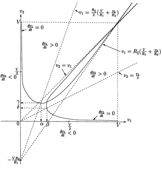
The equations (2.8) and (2.9) define two curves in the vI-v2 plane. Figure 2-2 is a plot

of these curves. The turning points of the two curves respectively are

(a0,Y)

yPR,2_-

_

(,6) = (2P 2R2, ,P 2R2) (2.11)

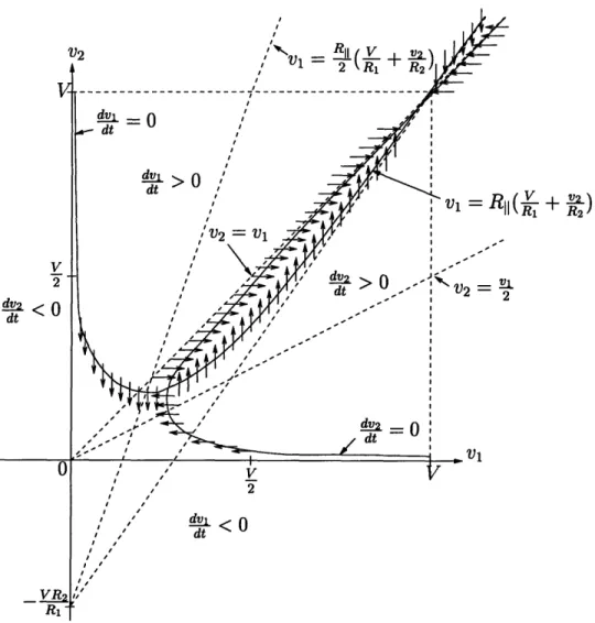
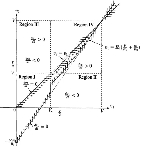
It is observed that there are two points of static equilibrium for the system; one point is near (V, V), while the other is closer to the origin. Graphically, the dynamics of the system can be represented as a vector field. Figure 2-3 shows the directions of the field along the

curve where R' = 0 and similarly along the curve where 42 = 0. For the given example,

it can be deduced from the direction of the field lines that the equilibrium nearer to (V, V) is stable while the one near the origin is not.

There can also exist configurations of parameters for which the two curves do not in-tersect and there is no real solution to (2.8) and (2.9). Physically, this represents a situation where the current drawn by the loads is so large that the current supplied by the source cannot ever charge up the capacitors, and hence the equilibrium state will be one where all nodal voltages are stuck at zero. In practice, this is not a particularly interesting or desir-able situation. For the remainder of this chapter, we will assume that the system is such that (2.8) and (2.9) have a pair of real solutions.

4~~> , I' V2 = v1 di I -I / to dt

Figure 2-2: Plot of i 1 = 0 and b2 = 0 loci for second-order system.

2.2 Gradient System Representation

In this section, we demonstrate that it is possible to express a RCP second-order system as a gradient system [2, 3]. Such a system has many well-understood properties which are useful in characterizing the dynamics and stability properties of the system.

V 2 d _dt <0 I dv.t- 0 dt di "V =V , r \'~ - I -I di I I I I I I I I I I dt <0

Figure 2-3: Vector fields for second-order system.

2.2.1 Gradient System

Definition

We begin with the definition of a gradient system. defined by

dv

dt = -grad E(v)

A gradient system is a vector field

(2.12) Ri R2 I I I V II~'"vl = ~( R, L

where E(v) is a scalar function referred to as the energy function and grad E(v) is defined by the following fundamental equality:

dE = < grad E(v), dv>

with < x, y > denoting an inner product for the vectors x and y. The rate of change of

E(v) along the field is given by

E(v)

= -|grad E(v) |2'

(2.13)

(2.14)

so,

E(v)

E(v)

Weighted Euclidean Inner Product

For the models in of this thesis, we need to use the following weighted Euclidean inner product for the definition of the gradient:

Ci > 0 for all i (2.15)

<x, y > = Cixiyi,

i=1

We can verify that this constitutes a valid inner product since the following properties are satisfied: <ax+/3y, z> <x, y> <x, x> > 0

= a<x,

With this definition,

grad E(v) = 1dE

where C =

C1 0

0 C2

If C is the identity matrix, the inner product reduces to the usual Euclidean inner product, and the definition of the gradient becomes the conventional one.

2.2.2

Energy Function for Ideal Loads

Consider the second-order system with ideal loads as described in Section 2.1. First, we rewrite (2.5) and (2.7) as dvl dt dv2 C2 dt

_dt

+

(

)

v

Our goal is to express (2.17) and (2.18) in the following form, for an appropriate E(vl, v2):

dvl dt dv2 C2 dt

_dt

E(v, v2) = -E(vi, v2)

f

Cdvl

J

C

dv

1

R,

-

+

P

ln(v

) + g(v1)

Matching f(v2) and g(vi) yields

V1 - VV _{P1 In(v)} -- R--1v l --12-+'P2-ln1-Pl(2.23) 2 1 2 + 2R2 v2 P ln(vi) + f(v2) (2.21) (2.22) V2 )V -R2 1 E(vl, V2) 2R _z!•llV

+

In(v2)

Hence, we can write the system of equations as dv dE C = d- (v) - (2.24) dt dv where C= 1 v=

Comparing (2.16) and (2.24), we conclude that

dv_{d = -grad E(v)}

(2.25)

which shows that that this second-order system is in fact a gradient system with respect to a weighted Euclidean inner product. If the capacitances C1 and C2 are equal, the system reduces to an ordinary Euclidean system where flow lines are normal to the level surfaces; if the capacitances C1 and C2 are not equal, the flow lines are normal to the level surfaces in the generalized sense defined by (2.15).

2.2.3 Energy Function for Non-Ideal Loads

The derivation of the results in the previous section assumed that the constant-power loads in the system were ideal, but a small modification yields the energy function for a system with non-ideal loads. We define

KI(vl) =

{

1,

vl > Vi* > 0

(2.26)

S0,

K2(v

) =

{

V2 > V2* > 0

(2.27)

S0,

where V,* and V2* are the cutoff voltages for the first and second loads respectively. Then

notice that Ki(vI) and ) are exactly the currents flowing through the two loads for all

KV, we can repeat our earlier derivation to conclude that now

V2

1 1 2 V v1v2 vl V2

E(vi,

v

2

)

= •

l

+

v2

-

vl -

+

Ki(vL)

In(•

) + K

(v)

In( )

(2.28)

It is easily verified that the energy function remains continuous at the cutoff boundaries, although its gradient is discontinuous at the boundaries.

With this modification to E(v), the equation

dE(v)

d- = -grad E(v)

dt

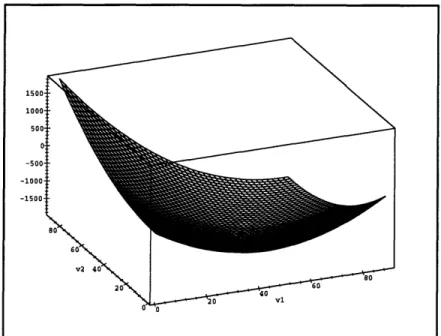
holds even for a system with non-ideal loads, except that a more detailed analysis is re-quired at the cutoff boundaries. Figures 2-4 and 2-5 show a 3-dimensional plot of an example of a typical energy function from two different angles.

Figure 2-5: Example plot of E(vl, v2) (different angle).

2.2.4 Application

The fact that the system is a gradient system allows us to draw several conclusions about the system [2, 3]. For example, in any region in which the energy function has continuous second-order partial derivatives, any (strict) local minimum of E(v) is an asymptotically stable equilibrium point of the system.

It is also possible to characterize the equilibria of the system by examining the Hessian (i.e. the matrix of second partial derivatives) of the energy function, as long as the equi-libria are not on the boundary lines defined by the cutoff voltages. Although our energy function is non-differentiable at these boundary lines, it is continuously twice-differentiable everywhere else in the region 0 < vl < V, 0 < v2 < V.

Consider a regular second-order system with identical components, i.e. R1 = R2 = R,

P1 = P2 = P and C1 = C2 = C, and identical cutoff voltages of V, for both loads. From

V, < vl < V, V, < v2 < V is given by

d

(v) - 1dv dv v- 1 R (2.30)

dv ₂ d2E d2E 1 P 1

dv2dvl V 2

Jv

R

Note that for vl > V,, v2 > V, we have

d2_{E d}2_E

dv2 _{(V, v}

2) - dv2 (Vc, Vc) > 0 (2.31)

where '> 0' here denotes positive definiteness, and the notation d2(V, V) is used to

denote the rightmost matrix in (2.30) evaluated at vl = V½, v2 = V,, but not to imply that

this is actually the Hessian of E(v) at vl = v2 = V,. Hence if

d2E (V, VC) > 0, _(2.32)

dv2

then any equilibria in the region vl > Vc, v2 > V, must be asymptotically stable, because

the matrix - d! (v) evaluated at any such equilibrium governs the small-signal dynamics at this equilibrium, and (2.31) and (2.32) together imply that - d (v) is negative definite, i.e. has all its eigenvalues real and negative. It is easy to show that any convex region where the Hessian is positive definite can have at most one equilibrium (which must be stable). The condition (2.32) is equivalent to requiring

P 1

-- + > 0, (2.33)

Vc2

R

P 2 ₍ P 1 1 > _o

V2

R

V2

R

R2

From inequality (2.34), we obtain

3

-

_V

V2

R<

_{2 P P}

The following condition therefore guarantees that for a regular second-order system with cutoff voltages set at V, any equilibrium in the box bounded by (Vc + e, Vc + c) and (V, V)

will be stable and unique:

2

v2 > PR (2.35)

There is also a possibility that equilibria may occur at the cutoff boundaries. These equilibria cannot be characterized by considering the Hessian of the energy function be-cause the function is non-differentiable at these points. In order to understand the dynamic behavior of the system at these points, more detailed analysis is required. The following section follows up on this analysis.

2.3 Boundary Behavior

In this section, we examine a second-order system much like the one discussed in the Section 2.1, but with the ideal constant-power loads replaced by non-ideal loads. To make the analysis more tractable, we assume that both loads have the same cutoff voltage, V,. Figure 2-1 is still the relevant circuit diagram for this discussion. For this analysis, we divide the v1-v2 plane into

4

Vc, v2 > V,} and {vi > VK, v2 > Ve}, and consider each of these cases separately.

Region I: vl < Vc, v2 < V,

In this region, both constant-power loads are in cutoff. The equivalent circuit is one with a voltage source V charging up the two capacitors, C1 and C2, through resistors R1 and R2.

The corresponding state equations are

dv₁ 1 R R RR d _ 1 (V - (1 _{+ .1)v1 +_. v2 (2.36)} dt C1R1 22.36) dv2 ₌ 1 (v1 - v2) (2.37) dt C2R2 40

Region II: vl > Vc, v2 < Ve

In this region, P1 is on, but P2 is still in cutoff. The corresponding state equations are

dv _ 1 V v₂ dVl - 1 (v 2 - ( + 2~ )V + PIRII₎ (2.38) dt C1Rivl R1 R2 dv2 _{= C}1 2R(vI - v2) (2.39)

dt

C2R2

In this region, P2 is on, but P1 is still in cutoff. The corresponding state equations are

dvldt _{dv =} CIR1 _- ( _{(1 +} R1 R 1) )Vl -+ RV2) _(2.40)

dt

C2

dt

In this region, both constant-power loads are functioning normally and the overall behavior of the system is identical to that of the system analyzed in Section 2.1. The corresponding state equations are (2.5) and (2.7).

Piecing together the dynamics in these four regions for an example of a second-order system, we obtain the phase-plane portrait shown in Figure 2-6. In this particular example, having a cutoff at Vc has effectively eliminated the unstable equilibrium point near the origin that was presented in Figure 2-3, creating a steady transition from zero initial state to the final stable equilibrium point. In order to more fully appreciate the effect of the cutoff voltage on the dynamics, it is essential to examine the boundary of the above regions of operation in more detail.

It is found that the steady state operating point for a second-order system is intrinsically tied to the behavior of the system at the cutoff boundaries vl = V, and v2 = V,. We analyze

Region III ei I

~i>o dt

(V + 2)

Figure 2-6: Phase-plane portrait for second-order system with cutoff.

the system in detail and find that the behavior of the system at a cutoff boundary is the limit of the behavior of the system on both sides of the boundary. More specifically, when the cutoff voltages of both loads are equal to V, it is possible for a dynamic equilibrium to occur on the boundary vl = V, iff

P

R

R2

Hence, to ensure that this does not happen, we require

P1R 1

V > + VC (2.43)

Similarly, it is possible for a dynamic equilibrium to occur on the boundary v2 = V iff

+

a

+

SR2 R _{< +}

_V

but we can prevent this if

P2R1R2 P1R1

V > V + + (2.45)

where RII = RR2 . For the case where Vc = , R1 = R2 = R and P1 = P2 = P, this

condition simplifies to

V2 _{> 4(1 + v3)PR (2.46)}

The details for these derivations are found in Appendix A.

The exact details of the derivations of the above conditions are not important. The es-sential point is that, through a detailed algebraic analysis of the dynamic behavior at the cutoff boundaries, we can derive sufficient conditions that guarantee that dynamic equilib-ria cannot exist for the system. However, this technique is not practical for higher-order systems. Later in Section 3.4.1, we will demonstrate that although the system is only a conventional gradient system in a piecewise sense, the system is well-behaved at the cut-off boundaries. In particular, the system satisfies the property that the energy function is monotonically decreasing with time even on the cutoff boundaries, if the system is not in equilibrium. This observation together with the fact that the energy function is lower bounded within W, the region of R2 such that 0 < vk < V for k = 1, 2, allow us to conclude that limit cycles cannot occur and the system must eventually settle at an equilib-rium. Hence, sufficient conditions to ensure that the system ends up at a desired equilibrium can be obtained simply from studying the steady-state behavior. We will demonstrate this

concept for the second-order case with identical cutoff voltages in the following section.

2.4 Steady-State Analysis

In Section 2.3 we derived general conditions that ensure a second-order system will not get stuck at the cutoff voltages of the loads by examining the dynamics of the system at the boundaries defined by the cutoff voltages. Here, for a regular second-order system where all the resistances, all the capacitances and all the loads are identical, we present an alternative approach that involves examining possible steady states. The circuit diagram for the system to be analyzed is given in Figure 2-7.

R R

P

Figure 2-7: Regular second-order system.

We will define an operational equilibrium as an equilibrium where all the constant-power loads are on. We begin with the assumption that the component values have been chosen such that there exists an operational equilibrium where vl > v2 > !. The

associ-ated equations are

2v2 - (V + v2)v1 + PR = 0 (2.47)

v - vIv2 + PR = 0 (2.48)

which we can solve to obtain

= V 2 + (V + v2 2 - (2.49)

4 16 2

v2 = - + - PR (2.50)

Since we know that the roots are real, the expressions under the square root signs must be positive. Hence,

v > 4PR, (2.51)

which implies V2 > 4PR, since V > vl.

We assume that both loads have cutoff voltage V,. We now attempt to find conditions on V, P, R and V, which will guarantee that the system cannot get stuck at the cutoff boundaries. If the system is in dynamic equilibrium, there are only two possible situations: either both vl is pinned at V or vl is operating above V, while v2 is pinned. In the former

case, since both cutoff voltages are equal and voltages are non-increasing with distance from the source, v2 is also pinned at V,.

Case I: v, = v2 = Vc Under these circumstances, il = VVc while i2 = 0. We next observe that if that ii > E = E, then this situation cannot occur. Hence, we impose the

condition V- V

_v-

_>

_P

_(2.52)

R

_½

Vc2- VV +PR < 0

(2.53)

Since V2 _{> 4PR, if}

½

Case II: v > v2 = Considering the current at the first node,

V - Vl P V1 v

V-

(2.58)

V V1 2 R V V1 -2 3V PR 8 2 9V 2 PR 64 2 V2 8 V2 V2 2P V 2PR V 2PR V V 2 2PR V V 8 PR PR V2

>

+

_V

> 4(1 + f)PR

Hence, if (2.66) holds and if the cutoff voltages are set at v, we can guarantee that the system cannot get stuck at the cutoff boundaries.

In summary, we have shown that under the following conditions:

* The resistances, capacitances and loads are identical,

* There exists an operational equilibrium such that vl > v2 > i,

* The cutoff voltages for both loads are set at !, and

* V2 _{> 4(1 + v)-)PR,}

a regular second-order ladder system is guaranteed to have all its equilibria constrained within P, the region of R2 such that E < Vk < V for k _{2 -} = 1, 2, not including its boundaries. If we compare this result with the sufficient condition for stability obtained in Section 2.3 (see equation (2.46)), we find that the results are identical. This is important because the

46 3V 8 (2.59) (2.60) (2.61) (2.62) (2.63) (2.64) (2.65) (2.66)

detailed analysis of the system dynamics at the boundaries is extremely involved and hence becomes impractical for higher-order systems. On the other hand, the results for this section can be generalized quite easily for higher-order systems.

In Section 3.2.2, we will prove that there must be at least one stable equilibrium in W, the region of R2 such that 0 < vk < V for k = 1, 2, and that all static equilibria must occur in P when the cutoff voltages for all loads are equal. We have shown that dynamic equilibrium cannot occur in W, and that there must be at least one stable equilibrium in P. So since the condition

V2 > PR (2.67)

as derived from (2.34) in Section 2.2.4 is satisfied, the operational equilibrium found is guaranteed to be globally stable and unique and the system is guaranteed to end up at this equilibrium starting from any initial conditions.

2.5

Summary of Results for Second-Order System

In summary, we have presented in this chapter the detailed analysis of a second-order RCP network. In general, a second-order system is found to have at most 2 equilibria, at least one of which is stable. We have also shown that it is possible to express a second-order system as a gradient system. From this fact, we know the the system is guaranteed to end up at an equilibrium in steady-state since there cannot be limit cycles. This is easy to see in the second-order case because the cutoff boundaries are straight lines which partition the phase-plane into 4 rectangular quadrants. We will show that this is true even for higher-order systems in Section 3.4.1.

Using the analytical properties of the gradient system, we can derive conditions for stability for a given equilibrium. In particular, for the second-order system shown in Fig-ure 2-7, where cutoffs voltages set at V, all equilibria in the box bounded by (V, + E, V, + c)

and (V, V) are guaranteed to be stable if

V > --2 5PR (2.68)

is satisfied.

Although the energy function fully characterizes the dynamic behavior of the system, the non-differentiability of the function at the cutoff voltages made the analysis of the behavior of the system at these points particularly tricky. After much detailed analysis of the system at these boundary points, it was found that in order to guarantee that a second-order system does not get stuck at these boundaries, the following stability condition must be satisfied:

P2R1R2 P1R1

V > VR+ + (2.69)

where R11 = R . In particular, for a regular second-order system with cutoff voltages

set at v, this condition simplifies to:

V2 _{> 4(1 + V/3)PR (2.70)}

Finally, a steady-state analysis was performed and it was found that we can relatively easily derive conditions that guarantee a second-order system does not get stuck at cutoff boundaries. The conditions obtained for a regular second-order system with cutoff voltages set at were found to be identical to those obtained with detailed boundary analysis. We conclude that steady-state analysis is a more practical way of obtaining simple sufficient conditions for stability, even though the results obtained by boundary analysis may possibly be more general.

Chapter 3

System Modeling and Dynamics:

Higher-Order Systems

In this chapter, we will generalize the results presented in Chapter 2 for higher-order sys-tems. We will demonstrate that any higher-order system can be expressed as a gradient system by presenting a method for constructing the energy function for a general RCP network. We showed in the previous chapter that both static and dynamic equilibria can exist. Here, we will discuss the identification and characterization of each of these types of equilibria in detail. Since the steady-state operating point of a network is completely determined by these equilibria, we present a general way of deriving simple sufficient con-ditions for system stability from the characterization of the equilibria. In particular, we derive specific results for regular RCP-ladder networks.

3.1 Gradient System Representation

In the previous chapter, we showed that we can express a second-order system as a gradient system. In fact, there is a systematic way to construct the energy function for any arbitrary network topology, as long as it satisfies some layout constraints. More specifically, each

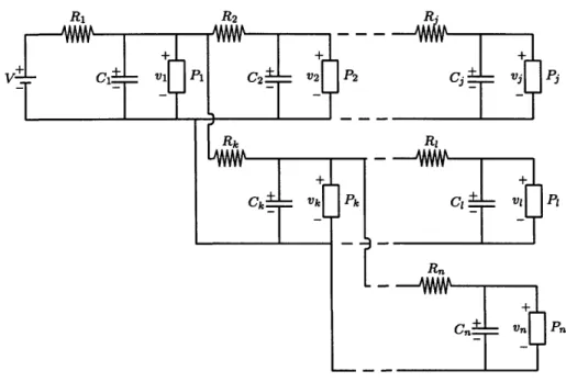
node in the network is connected to only one capacitor and one constant-power load, and all loads share a common ground connection. There is no constraint on the number of resistors attached to each node. Figure 3-1 is an example of an nth-order tree with branching that satisfies the above constraints.

Figure 3-1: An nth-order tree network with branching.

We can apply Kirchhoff's Current Law to find the current flowing through the capaci-tors. The system of equations obtained is of the following form:

dvk Kk (vk) +

z

fork

dt Vk RjER Rj

(3.1)

where Rk is the set of all resistors connected to node k and vk - Vj,k is the potential

difference across resistor Rj. Notice that if we define the partial sums

(3.2)

En

(

R.

then the energy function is simply given by

En(v) = En,k(v) (3.3)

k=l

Thus, the energy function of any arbitrary network takes the following form:

n Vk

1

En(v) = Kk(Vk)ln( ) + - )k - -VkVj,k) (3.4)

k=1 k k= RjER2k k=1 RjERk R

where Rk is the set of all resistors connected to node k and Vk - Vj,k is the potential

difference across resistor Rj. This is proved simply by partial differentiation of (3.4) which yields the negative of expressions of the form given on the right side of (3.1).

3.2 Characterizing Equilibria

In this section, we study the equilibria of a general higher-order system in detail. Let us first define W as the region of Rn such that 0 < vi < V for i = 1,..., n. It is easy to show

that W is the positive-invariant bounding box for the state of any higher-order system. The rationale here is that voltages cannot be negative and they also cannot exceed the source voltage. We show in this section that there is at least one stable equilibrium in W, and that all equilibria must be contained within W and cannot occur on the upper or lower

boundaries, i.e. where Vk = 0 or vk = V _{for some node k.}

3.2.1

Types of Equilibria

At this point, it is important to note that there are two classes of equilibria for RCP-tree networks: static (asymptotically stable and unstable) equilibria and dynamic (stable) equi-libria. In both cases, the voltages at the nodes of a system in equilibrium are constant in the absence of perturbation; the difference between these two classes of equilibria lies in the operating point of the constant-power loads.