Investigation of a sample of carbon-enhanced metal-poor stars observed with FORS and GMOS

(1)

HAL Id: hal-02308108

https://hal.archives-ouvertes.fr/hal-02308108

Submitted on 13 Nov 2020

HAL is a multi-disciplinary open access

archive for the deposit and dissemination of

sci-entific research documents, whether they are

pub-lished or not. The documents may come from

teaching and research institutions in France or

abroad, or from public or private research centers.

L’archive ouverte pluridisciplinaire HAL, est

destinée au dépôt et à la diffusion de documents

scientifiques de niveau recherche, publiés ou non,

émanant des établissements d’enseignement et de

recherche français ou étrangers, des laboratoires

publics ou privés.

Investigation of a sample of carbon-enhanced metal-poor

stars observed with FORS and GMOS

E. Caffau, A. Gallagher, P. Bonifacio, M. Spite, S. Duffau, F. Spite, L.

Monaco, L. Sbordone

To cite this version:

E. Caffau, A. Gallagher, P. Bonifacio, M. Spite, S. Duffau, et al.. Investigation of a sample of

carbon-enhanced metal-poor stars observed with FORS and GMOS. Astronomy and Astrophysics - A&A,

EDP Sciences, 2018, 614, pp.A68. �10.1051/0004-6361/201732475�. �hal-02308108�

(2)

Astronomy

_&

Astrophysics

A&A 614, A68 (2018)

https://doi.org/10.1051/0004-6361/201732475

Investigation of a sample of carbon-enhanced metal-poor stars

observed with FORS

?

_{and GMOS}

??

,

???

E. Caffau

1

_{, A. J. Gallagher}

2,1

_{, P. Bonifacio}

1

_{, M. Spite}

1

_{, S. Duffau}

3

_{, F. Spite}

1

_{, L. Monaco}

3

_{, and L. Sbordone}

4

1 _{GEPI, Observatoire de Paris, Université PSL, CNRS, 5 Place Jules Janssen, 92190 Meudon, France}

e-mail: elisabetta.caffau@obspm.fr

2 _{Max-Planck-Institut für Astronomie, Königstuhl 17, 69117 Heidelberg, Germany}

3 _{Departamento de Ciencias Fisicas, Universidad Andres Bello, Fernandez Concha 700, Las Condes, Santiago, Chile} 4 _{European Southern Observatory, Casilla 19001, Santiago, Chile}

Received 15 December 2017 / Accepted 16 February 2018

ABSTRACT

Aims. Carbon-enhanced metal-poor (CEMP) stars represent a sizeable fraction of all known metal-poor stars in the Galaxy. Their formation and composition remains a significant topic of investigation within the stellar astrophysics community.

Methods. We analysed a sample of low-resolution spectra of 30 dwarf stars, obtained using the visual and near UV FOcal Reducer and low dispersion Spectrograph for the Very Large Telescope (FORS/VLT) of the European Southern Observatory (ESO) and the Gemini Multi-Object Spectrographs (GMOS) at the GEMINI telescope, to derive their metallicity and carbon abundance.

Results. We derived C and Ca from all spectra, and Fe and Ba from the majority of the stars.

Conclusions. We have extended the population statistics of CEMP stars and have confirmed that in general, stars with a high C abundance belonging to the high C band show a high Ba-content (CEMP-s or -r/s), while stars with a normal C abundance or that are C-rich, but belong to the low C band, are normal in Ba (CEMP-no).

Key words. stars: Population II – stars: abundances – Galaxy: abundances – Galaxy: formation – Galaxy: halo

1. Introduction

The existence of stars with large carbon enhancement was sus-pected from the very beginning of astronomical spectroscopy.

In his “Memoria” of 1868, Angelo Secchi (Secchi 1868) added

a fourth spectral type to the three he defined earlier and noted that “not all the stars of the fourth type have identical spectra: this type allows a wider variety than the three previous ones. The black line after the green almost coincides with magnesium, but it may well be due to carbon. More precise measures will decide: its width makes us believe that it is not metallic”1_{. The}

“black line” observed by Secchi is indeed the C2 Swan band

that characterises carbon stars, i.e. stars that have C/O2> 1, see ?_{Based on observations made with ESO Telescopes at the La Silla}

Paranal Observatory under programme ID 099.D-0791.

??

Based on observations obtained at the Gemini Observatory (pro-cessed using the Gemini IRAF package), which is operated by the Association of Universities for Research in Astronomy, Inc., under a cooperative agreement with the NSF on behalf of the Gemini part-nership: the National Science Foundation (United States), the National Research Council (Canada), CONICYT (Chile), Ministerio de Ciencia, Tecnología e Innovación Productiva (Argentina), and Ministério da Ciência, Tecnologia e Inovação (Brazil).

???

Tables 1 and 2 are also available at the CDS via

anony-mous ftp to cdsarc.u-strasbg.fr (130.79.128.5) or via

http://cdsarc.u-strasbg.fr/viz-bin/qcat?J/A+A/614/A68

1 _{Original text in Italian: “Non tutte le stelle del 4}◦

tipo sono di spettro identico: questo tipo ammette varietà maggiori che i tre precedenti. La riga nera dopo il verde coincide quasi con il magnesio, ma può bene anche appartenere al carbonio. Le misure più precise decideranno: la sua larghezza ci fa credere che non è la metallica”.

2 _X/Y_{= N(X)/N(Y) = 10}[A(X)∗−A(Y)∗]_.

McCarthy(1994) for more details on Secchi’s discovery and a modern identification of his type 4 stars. It is remarkable that at the low resolution of his prism spectra, Secchi was able to sus-pect that the line was too wide to be an atomic line; this proves that Secchi was an exceptional observer.

In what can be considered a milestone review, Bidelman

(1956) introduced the class of “non-typical” carbon stars, and

among these the “CH stars” that show “extremely strong features due to CH, and considerably weaker lines of neutral metals than do the “typical” carbon stars”. This was the first class of metal-poor carbon-enhanced stars to be clearly identified, although

they are only “mildly” metal poor ([Fe/H] >∼ −1.5). As soon

as it was possible to determine detailed chemical abundances, it became clear that the composition of carbon stars was the result of nuclear processing; this concept is well explained in

the influential review byWallerstein(1973). At the time it was

unclear, however, whether this processing took place in the star itself (self-pollution) or if it was the result of mass transfer from an evolved companion. By the mid-1990s, the general consensus was that Ba stars, CH-stars, and sg-CH-stars were the

result of mass transfer in a binary system (McClure 1984,1997,

McClure & Woodsworth 1990). During its lifetime, the higher mass star of the binary system evolves onto the asymptotic giant branch (AGB), where it is fuelled in part by helium burning, producing freshly synthesised carbon and dredging it up to its atmosphere through several convective mechanisms, induced by thermal pulsations. The giant star atmosphere then expands and becomes tenuous, exceeding its Roche lobe or even encompassing the lower mass companion in the case of close binary systems. This allows accretion of the atmosphere of the

A68, page 1 of10

Open Access article,published by EDP Sciences, under the terms of the Creative Commons Attribution License (http://creativecommons.org/licenses/by/4.0), which permits unrestricted use, distribution, and reproduction in any medium, provided the original work is properly cited.

(3)

higher mass star, which contains freshly synthesised carbon, by the lower mass star.

The HK survey (Beers et al. 1985,1992) was aimed at the

discovery of metal-poor stars. One of the first surprising results was that about 10% of the stars with an estimated metallic-ity below –2.0 showed a G-band stronger than normal, while at higher metallicity, strong G-band stars were less frequent (Norris et al. 1997a). The first handful of strong G-band stars from the HK Survey that were analysed at high resolution proved

to be enhanced in the s-process elements (Barbuy et al. 1997;

Norris et al. 1997a), and the exceptional star CS 22892-052

proved to be also enhanced in r-process elements (McWilliam

et al. 1995; Sneden et al. 1996). This was a strong suggestion that these stars are indeed metal-poor analogues of CH-stars and the result of mass-transfer in a binary system. The

situa-tion changed drastically with the study of CS 22957-027 (Norris

et al. 1997b; Bonifacio et al. 1998), which showed a large

C-enhancement and a very strong Swan band (Bonifacio et al.

1998), but no enhancement of any of the neutron capture

ele-ments. In order to distinguish these stars from the classical carbon stars and CH-stars, it soon become customary to refer to them as carbon-enhanced metal-poor stars (CEMP, for short); the first two occurrences of the acronym in the literature are in

Lucatello et al.(2003) and in the review byChristlieb(2003).

We take the definition of Beers & Christlieb (2005), and

consider a metal-poor star as a CEMP when [Fe/H] <∼ −2.0 dex

and [C/Fe] > +1.0 dex. When a CEMP star is also enhanced

in s−process elements, we refer to it as a CEMP-s star,

i.e. [C/Fe] > +1.0, [Ba/Fe] > +1.0 and [Ba/Eu] > +0.5

(Beers & Christlieb 2005). Another sub-class of CEMP stars show enhancements in both slow (s-) and rapid (r-) process material, such that [C/Fe] > +1.0 and 0.0 < [Ba/Eu] < +0.5 (Beers & Christlieb 2005). These stars are referred to as CEMP-r/s stars. Like CEMP-s stars, a large fraction of CEMP-r/s stars are found in binary systems, explaining their car-bon and s-process enhancements. The r-process enhancement is peculiar, however. It has been suggested that these stars undergo

a double-enhancement phase (Jonsell et al. 2006;Bisterzo et al.

2006). The s-process and carbon enhancement still occurs due

to binary interaction, but the r-process enhancement takes place in the forming gas cloud, when it is enriched by r-process

material. Since the discovery of GW170817 (Troja et al. 2017),

observational evidence suggests that the main sites for the r-process are neutron star mergers. The r-process-rich ejecta from these events mix with the interstellar medium (ISM), which will become star-forming regions and form new generations of

r-rich stars. Moreover, Hampel et al. (2016) could explain the

pattern of the heavy element abundances in 20 CEMP-rs stars by the accretion of the products of the i-process (Cowan & Rose

1977) occuring in the intershell region of low-metallicity AGB

stars.

CEMP-s (and CEMP-r/s) stars are the most commonly found sub-class of CEMP stars, making up approximately 80%

of all CEMP stars known (Aoki et al. 2007, 2008). It is

now well established that the CEMP-s stars are all members

of binary systems (Lucatello et al. 2005; Starkenburg et al.

2014). However, some CEMP stars appear to be similar to

the prototype star CS 22957-027 and show no other enhance-ments. These stars are known as CEMP-no stars ([C/Fe] > +1.0, [Ba/Fe] < 0.0 Beers & Christlieb 2005). Additionally, there is currently no evidence that supports an unusually high fraction of binarity in these objects, but only a handful of these objects have radial velocity measurements at this time

(e.g. the ultra Fe-poor star by Caffau et al. 2016). This would

suggest that accretion through binary interaction is proba-bly not the means by which these stars attained their carbon enhancement. Therefore, these stars would appear to exhibit abundance patterns indicative of the gas cloud from which they formed, making their unusual chemical composition a mystery.

Spite et al.(2013) suggested that CEMP stars are divided into

two groups: the high C band and the low C band.Bonifacio et al.

(2015) argued for a different origin of the two groups, where the stars of the higher band are members of a binary system and those that belong to the low band present the composition of the gas cloud from where they have formed, as described above.

Further thoughts on the two C bands are discussed byBonifacio

et al.(2018). In the case of dwarf CEMP stars, when they are extremely metal poor, it is in general not easy to detect any sign of heavy elements. The most Fe-poor stars known belong to the low C band, while the stars in the high C band rarely have [Fe/H] <∼ −3.5 dex.Bonifacio et al.(2018) proposed a clas-sification for the stars on the two C bands according their C abundance, regardless of their abundances in neutron capture elements.

We present an analysis made on a sample of stars observed at low resolution with the visual and near UV FOcal Reducer and low dispersion Spectrograph for the Very Large Telescope (FORS/VLT) of the European Southern Observatory (ESO) and the Gemini Multi-Object Spectrographs (GMOS) at the GEMINI telescope, in the following study, and examine, among other things, their carbon abundances.

2. Observations and data reduction

The spectra presented in this paper have been acquired in the course of two programs approved by the ESO and GEMINI observatories. The programs have been designed to be “filler” programs, meaning that they can acquire useful data in weather conditions when most programs cannot operate and have no con-straint on the Moon phase. Our spectra have been acquired with

FORS (Appenzeller et al. 1998) at the ESO VLT 8.2 m

tele-scope and with GMOS (Hook et al. 2004) at the GEMINI 8.2 m

telescope.

The FORS spectra have been observed in service mode dur-ing the ESO Programme 099.D-0791, between 01/04/2017 and 16/08/2017. We used GRIS 1200B with a central wavelength of

436 nm and a slit width of 0.00_{29, which provides a resolving}

power R ∼ 5000 at the central wavelength and a continuous spectral coverage in the range 366 nm to 511 nm. The detec-tor used was the CCD mosaic of two 2k × 4k MIT CCDs with pixel size of 15 µm. The detectors are arranged in a line in the direction orthogonal to the dispersion, thus there are no gaps in the spectra. This mosaic is more sensitive in the red; using the blue sensitive mosaic of E2V CCDs would have been more efficient, but this detector camera is normally not mounted on FORS. Since the program was designed as a “filler” program, we had to use the default detector. We initially began the observa-tions with a 2 × 2 on-chip binning, that is, the default for FORS, which is supposed to be used for service observations. We knew that in this way, the spectrum would be under-sampled in the blue part, but our primary goal was the G-band, which is very wide and thus would not be under-sampled; the same applies to the CaIIK line.

We acquired spectra for eight stars in this configuration

(SDSS J0905+0330, SDSS J1248–0726, SDSS J1313–0019,

SDSS J1349–0229, SDSS J1411+0503, SDSS J2137–0057,

SDSS J2219+0515, and SDSS J2239–0048). As soon as the

(4)

E. Caffau et al.: FORS/GMOS sample

spectra were observed, they were reduced with the ESO FORS

pipeline3 driven by gasgano4. They were subsequently analysed

with MyGIsFOS (Sbordone et al. 2014). At this point, we

realised that several FeI lines could be used in the blue part

of the spectrum and that the under-sampling introduced an undesirable increase in the uncertainty. We therefore submitted to ESO a waiver request to be allowed to use the 1 × 1 bin-ning even in service mode. The waiver was approved and all subsequent observations were acquired with a 1 × 1 binning. For each star we used an observing block of 1 h. For the 2 × 2 binning, this translates into an effective exposure time of 2829 s. For the 1 × 1 binning, since the read-out time is longer, this translates into 2762 s of exposure time. Thirty spectra of quality A or B and one spectrum with quality C have been retained for analysis for a total of 28 stars. Star SDSS J144533.32–004559.0 had two “B” quality spectra, each of which was analysed independently.

The GMOS spectra were acquired in service mode on the nights of 21/07/2017 and 25/07/2017. We used the

B1200+_G5321 grating centred at 468 nm, with a slit of 0.005.

This combination provides a resolving power R = 3744 at the

blaze wavelength (463 nm) and a spectral coverage from 387 nm to 548 nm. The detector was a mosaic of three Hamamatsu

2 k × 4 k CCDs with pixels of 15 µm side (Gimeno et al. 2016).

The three detectors are arranged in a line along the disper-sion direction, which implies that there are two gaps in the wavelength range. The gap ranges are 438.7−440.8 nm and 493.0−495.1 nm. We used a 2 × 2 binning, which is the default. For each star we observed three exposures of 441 s. The data

were processed with GEMINI IRAF5_package6_{, to perform bias}

subtraction, flat-fielding, and mosaicking of the different

sub-images. We then used the ESO MIDAS7LONG context to perform

the wavelength calibration using the CuAr lamp spectra and the optimal extraction (including sky-subtraction). The three exposures for each star where then added and analysed with MyGIsFOS.

3. Sample

We selected a sample of turn-off stars from the Sloan Digital Sky

Survey (SDSS;York et al. 2000; Yanny et al. 2009) that were

bright enough (g < 17) to allow us to secure a reasonable spec-trum quality in a single observing block of 1 h. To select turn-off

stars on the SDSS, we requested 0.18 ≤ (g − z)0 ≤ 0.70 and

(u −g)₀ > 0.70 (seeCaffau et al. 2013b) and obtained a sample of about 20 000 stars observable from Paranal. By examining our own analysis of the SDSS spectra, we focused on stars for which we derived a metallicity in the range −3.0 < [Fe/H] < −0.5 and that also exhibited a strong G-band features. This meant

that stars that potentially belonged to either C bands (Spite

et al. 2013) were selected, as well as stars at the metal-rich end of the two C bands – “normal” stars, with a solar-scaled C abundance.

Table1 lists the stars we examined here, along with their

coordinates, g-mag, and metallicities derived from Fe abun-dances computed using SDSS and FORS/GMOS spectra.

3 _{ftp://ftp.eso.org/pub/dfs/pipelines/fors/} fors-kit-5.3.23.tar.gz 4 _{ftp://ftp.eso.org/pub/dfs/gasgano/} gasgano-2.4.8.tar.gz 5 _{http://iraf.noao.edu/} 6 _{http://www.gemini.edu/node/11823} 7 _{https://www.eso.org/sci/software/esomidas/} 4. Analysis 4.1. Comparison FORS/GMOS - SDSS

In the FORS and GMOS spectra, several FeIlines are usually

available to derive A(Fe) (and also [Fe/H]). However, we were not able to derive a direct Fe abundance for three stars (SDSS J2219+0515, SDSS J1149+0723, and SDSS J1349–0229) because no clean Fe line was available in their spectra. Instead, we provide an estimation of A(Fe) based on comparison of syn-thetic spectra and observed on the full spectral range. For these stars, the σ related to the iron abundance is an estimation of the uncertainty in this comparison.

The SDSS spectra are of lower resolution, and in this case, we derive the metallicity, [M/H], from any available metallic fea-ture in the spectra, so that the metallicity is usually based on Ca, Mg, and Fe abundances. The synthetic spectra we used for the chemical investigation of the SDSS spectra are enhanced in α elements by +0.4 dex in the metal-poor regime, as normally expected in Galactic metal-poor stars. So the scale provided to give the metallicity, [M/H], is related to the Fe abundance. This is reasonable for “normal” stars that do not show peculiar [Mg/Fe] or [Ca/Fe] ratios, which seems to be mainly the case

in this sample of stars. In Table1 we list the [Fe/H] derived

from the FORS and GMOS spectra and the [M/H] from the SDSS spectra. The comparison is generally very good, but there are some exceptions that we discuss below. When multiple SDSS spectra of comparable quality were available, the

metal-licity and the uncertainty listed in Table1represent an average

value.

Nineteen of the 27 stars in the sample present absolute differ-ences in the metallicity derived from SDSS and the iron content from the FORS and GMOS spectra lower than 0.3 dex, and for 22 stars, this is lower than 0.5 dex. For all but three spectra (SDSS J1349–0229, SDSS J2137–0057, and SDSS J1411+0503), the metallicity from SDSS and [Fe/H] from FORS/GMOS spec-tra agree within the uncertainties.

We present some of the more interesting facts about a small

number of the stars we analysed in Table1.

– SDSS J1349–0229 shows the largest difference in metallicity when the FORS and SDSS spectra are analysed. Two spec-tra are available in SDSS DR12, providing a large difference among themselves in metallicity of 0.65 dex. For one of them,

the metallicity is based on a single line. We report in Table1

the metallicity derived from the other SDSS spectrum, based on four features, still with a large uncertainty. In addition, the qual-ity of the FORS spectrum is not good (classified as “C”) and is the poorest FORS spectrum in our sample. The difference in the [M/H] from the best SDSS spectrum and [Fe/H] from the FORS spectrum is 1.44 dex, just larger than the sum of the two uncertainties (1.38 dex). SDSSJ1349–0229 was also analysed by

Behara et al.(2010) with a temperature only 62 K hotter than the

value given in Table2. We derived from the FORS spectra the

same Fe abundance asBehara et al.(2010), and we consider the

results of the two analyses in very good agreement.

– The metallicity and [Fe/H] derived from SDSS and FORS spectra, respectively, for SDSS J2137–0057 differ by 0.63 dex, but the uncertainties are 0.60 dex, so the agreement is acceptable.

– The difference in metallicity and [Fe/H] in SDSS J1411+0503 from SDSS and FORS spectra is 0.8 dex with uncertainties of 0.62 dex. The SDSS analysis is based on two spectra, provid-ing metallicities within 0.01 dex, and the uncertainty is 0.4 and

0.3 dex for the two spectra. One SDSS spectrum has no CaII-K,

(5)

Table 1. Sample of stars.

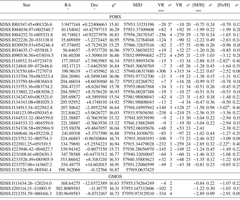
Star RA Dec ga _MJD _{VR σ VR} _{σ [M/H] σ [Fe/H] σ}

◦ ◦ SDSS SDSS FORS SDSS J001547.45+001326.6 3.9477144 +0.22406663 15.81 57953.33251196 −20 2a _{−10 20 −0.75 0.24} _{−0.70 0.17} SDSS J004036.97+002540.7 10.154042 +0.42797715 16.29 57953.37109608 +82 3 +92 19 −1.99 0.22 −1.99 0.21 SDSS J004252.51+005521.8 10.718813 +0.92273976 16.83 57956.28170347 −256 4 −270 29 −1.70 0.24 −1.65 0.13 SDSS J022226.20–031338.0 35.609189 –3.2272445 16.95 57956.32784048 −124 3 −90 32 −2.22 0.49 −2.63 0.24 SDSS J030929.93+054246.4 47.374692 +5.7129120 15.25 57966.32655116 −82 2 −57 35 −0.96 0.26 −0.96 0.16 SDSS J034635.17–055818.3 56.64657 –5.9717720 16.96 57973.36030252 +19 2 +32 27 −1.20 0.26 −0.85 0.19 SDSS J090536.50+033034.5 136.40208 +3.5096110 16.86 57852.99994682 +272 4 +295 21 −2.19 1.03 −3.12 0.21 SDSS J114932.51+072347.0 177.38547 +7.3963985 16.34 57953.98955476 −15 3 −33 34 −2.88 0.15 −2.82b_{: 0.40} SDSS J124841.09–072646.6 192.17123 –7.4462930 16.84 57845.30650769 −7 3 −45 26 −1.28 0.45 −1.64 0.39 SDSS J131550.68+172707.0 198.96119 +17.451962 16.12 57940.06317480 +306 3 +315 34 −2.22 0.67 −2.52 0.06 SDSS J133704.70+083523.4 204.26961 +8.5898340 16.06 57951.97732700 −21 3 −19 23 −1.38 0.15 −1.31 0.17 SDSS J133750.48+083610.8 204.46034 +8.6030160 16.72 57952.02268752 +7 3 +16 28 −0.99 0.37 −0.78 0.18 SDSS J133753.36+083734.2 204.47237 +8.6261760 15.78 57955.06167568 −34 3 −11 34 −0.51 0.26 −0.45 0.25 SDSS J133802.22+083056.2 204.50927 +8.5156120 16.93 57956.00287188 −19 3 −10 27 −0.51 0.51 −0.53 0.18 SDSS J134247.69+083521.0 205.69872 +8.5891910 15.54 57981.98808043 −42 4 −23 31 −1.63 0.18 −1.48 0.23 SDSS J134343.08+081029.3 205.92952 +8.1748110 14.92 57981.98808043 −13 2 −4 34 −0.47 0.36 −0.50 0.22 SDSS J134913.54–022942.8 207.30642 –2.4952258 16.64 57916.14995942 +140 3 +128 27 −1.58 0.98 −3.02b_{: 0.40} SDSS J141123.09+050345.6 212.84622 +5.0626727 16.03 57933.97656561 −238 4 −210 25 −2.56 0.35 −3.36 0.27 SDSS J144533.32–004559.0 221.38887 –0.7663930 15.32 57941.10539190 −9 2 −13 30 −3.04 0.22 −2.94 0.19 SDSS J144533.32–004559.0 221.38887 –0.7663930 15.32 57941.13882949 −9 2 −19 30 −3.04 0.22 −2.94 0.19 SDSS J154338.58+092904.9 235.91078 +9.4847057 16.04 57952.06105676 +48 2 +53 23 −2.41 −2.38 0.23 SDSS J160646.36+052218.2 241.69318 +5.3717390 16.88 57954.10306751 −85 3 −97 22 −1.02 0.44 −1.27 0.29 SDSS J213752.52–005754.3 324.46883 –0.96510684 16.74 57915.30185193 −108 5 −73 23 −2.46 0.52 −3.09 0.08 SDSS J221911.25+051519.5 334.79691 +5.2554223 16.94 57915.34479028 −232 3 −259 24 −2.85 0.32 −2.22b_{: 0.40} SDSS J223946.42–004827.7 339.94342 –0.8077150 15.73 57938.28656970 −145 2 −149 22 −1.24 0.45 −1.49 0.22 SDSS J231108.61+002650.3 347.78588 +0.44731512 16.77 57940.32010047 −64 3 −60 21 −1.46 0.32 −1.68 0.27 SDSS J233526.49+081905.9 353.86042 +8.3183210 16.53 57940.35885623 +32 3 +48 23 −1.35 0.12 −1.22 0.19 SDSS J233757.06+143607.2 354.48775 +14.602015 16.91 57951.22060599 −49 2 −43 38 −0.81 0.23 −0.85 0.23 SDSS J131326.89–001941.4 198.362066 –0.32766 16.87 57919.0637425 GMOS SDSS J111434.26–120214.0 168.64275 –12.0372389 16.63 57955.174264249 −4 2 −0.84 0.22 −1.07 0.22 SDSS J201114.15–111003.9 302.8089583 –11.16775 16.31 57955.147332606 −102 2 −1.22 0.30 −1.03 0.17 SDSS J212351.59–080416.3 320.9649583 –8.0712167 16.73 57959.973129110 −334 4 −2.89 0.09 −2.91 0.09

Notes. [M/H] from SDSS is based on several metallic features; [Fe/H] from FORS and GMOS spectra are taken from FeIlines only. The solar A(Fe) = 7.52 adopted is taken fromCaffau et al.(2011). The σ are line-to-line scatter, and for the uncertain cases, the colon in the iron abundance is an estimate of the uncertainty in the comparison to synthetic spectra.(a)_{g magnitudes are those used to derive the effective temperatures and are}

taken from the SDSS-DR 12.(b)_{Estimation from comparison to synthetic spectra; we consider these measurements to be uncertain.} but other features are present. The 0.8 dex difference from SDSS

and FORS spectra is just larger than 1σ, so we find it acceptable. – For the star SDSS J2219+0515, there is a 0.63 dex difference between the metallicity derived from the SDSS spectrum and [Fe/H] derived from the FORS spectrum (which falls within the uncertainties of the two measurements) that can be explained by no-clean Fe line in the FORS spectrum. The A(Ca) value derived from the FORS data is in perfect agreement with the SDSS anal-ysis.

– For SDSS J0905+0330, the metallicity derived from the SDSS spectrum has a large uncertainty (1 dex) and is based on only two features; as a consequence, the 0.93 dex differ-ence with the [Fe/H] from the FORS spectrum is well within 1σ.

– For the stars SDSS J0346–0558 and SDSS J1248–0726, Gaia (Gaia Collaboration 2016) detected another source, 1.21 mag fainter, at distances of 5 arcsec and 4 arcsec, respec-tively. The difference in flux from our target star and the other

object is in both cases large enough to avoid compromising our analysis.

– SDSS J2011–1110: two objects are detected by Gaia within 2 arcsec, with a difference in the Gaia mag of 2.53. The two objects are very close, but the fainter star is too faint to interfere with the signal from our target.

– SDSS J1315+1727, SDSS J1337+0836, SDSS J1337+0836, SDSS J1337+0837, and SDSS J1343+0810 have a 2MASS identification.

4.2. Radial velocities

The radial velocities have been derived with the cross-correlation of each spectrum with a synthetic spectrum with very simi-lar parameters, also taking into account the C enhancement of the star. We are aware that FORS suffers from the telescope flexions, which makes the radial velocity measurements uncer-tain. We took into account the position of the stars in the sky

(6)

E. Caffau et al.: FORS/GMOS sample Table 2. Derived abundances.

Star Teff A(Fe) A(FeII) A(C) 3Dcor A(Mg) A(Si) A(CaK)/A(Ca) A(Ti) A(Mn) A(Sr) A(Ba)

SDSSJ0015+0013 6065 6.82 ± 0.17 7.03 ± 0.18 7.82 −0.03 7.28 7.22 5.81/6.01 ± 0.21 4.45 ± 0.20 4.79 ± 0.21 1.74 SDSSJ0040+0025 5651 5.53 ± 0.21 6.53 −0.15 6.02 4.76/4.64 ± 0.18 3.14 ± 0.27 3.62 ± 0.24 0.46 0.54 SDSSJ0042+0055 6019 5.87 ± 0.13 6.79 −0.15 6.34 5.21/5.03 ± 0.15 3.75 ± 0.17 3.77 ± 0.08 1.67 1.35 SDSSJ0222–0313 6345 4.89 ± 0.24 8.08 −0.08 4.11/4.12 ± 0.30 3.17 ± 0.01 2.54 1.52 SDSSJ0309+0542 6012 6.56 ± 0.16 6.36 ± 0.20 7.74 +0.05 7.17 5.71/5.73 ± 0.22 4.42 ± 0.32 4.49 ± 0.14 2.02 1.15 SDSSJ0346–0558 5660 6.67 ± 0.19 6.51 ± 0.19 7.61 +0.10 7.06 5.62/5.55 ± 0.06 4.27 ± 0.25 4.74 ± 0.30 2.00: 1.50 SDSSJ0905+0330 6263 4.40 ± 0.27 7.68 −0.15 3.99/3.52 ± 0.30 0.40: 1.47: SDSSJ1149+0723 6000 4.7 ± 0.40: 7.66 −0.05 3.86/3.70 ± 0.30 2.50 ± 0.30 <1.0 0.30: SDSSJ1248–0726 6234 5.88 ± 0.39 7.94 −0.10 6.40 4.99/5.09 ± 0.32 3.62 ± 0.13 4.09 ± 0.30 2.64 3.05 SDSSJ1315+1727 6170 5.00 ± 0.06 8.34 −0.05 3.99 0.30: 1.81 SDSSJ1337+0835 6023 6.21 ± 0.17 7.35 +0.00 6.91 5.38/5.39 ± 0.13 3.74 ± 0.28 4.19 ± 0.18 1.80 0.90 SDSSJ1337+0836 5970 6.74 ± 0.18 8.44 +0.15 7.18 6.27/6.00 ± 0.38 4.32 ± 0.18 4.39 ± 0.30 1.90 SDSSJ1337+0837 5464 7.07 ± 0.25 8.10 +0.15 6.09/6.22 ± 0.24 4.46 ± 0.28 4.88 ± 0.31 1.82 SDSSJ1338+0830 5496 6.99 ± 0.18 8.04 +0.15 7.61 6.02/6.10 ± 0.26 4.72 ± 0.23 4.94 ± 0.24 1.67: SDSSJ1342+0835 6176 6.04 ± 0.23 7.00: −0.10 5.21/4.91 ± 0.16 3.89 ± 0.24 3.68 ± 0.30 1.85 0.51 SDSSJ1343+0810 5482 7.02 ± 0.22 7.97 +0.15 7.45 7.37 6.03/6.02 ± 0.07 4.72 ± 0.16 5.33 ± 0.14 1.72 SDSSJ1349–0229 6138 4.5 ± 0.40: 8.32 +0.00 3.78 1.00: 1.50 SDSSJ1411+0503 5930 4.16 ± 0.23 6.86 −0.15 3.91 −0.19 <−0.8 SDSSJ1445–0045,2 5492 4.58 ± 0.19 6.18 −0.15 3.64/3.30 ± 0.30 2.65 ± 0.26 −0.12 <−1.0 SDSSJ1445–0045,1 5492 4.49 ± 0.21 6.18 −0.15 3.63/3.49 ± 0.29 2.53 ± 0.06 −0.34 <−1.0 SDSSJ1543+0929 6288 5.14 ± 0.08 8.42 −0.05 4.05 1.13: 1.21: SDSSJ1606+0522 6122 6.25 ± 0.29 6.55 7.81 +0.00 6.58 5.38/5.69 ± 0.01 4.59 ± 0.04 3.29 2.95 SDSSJ2137–0057 5956 4.43 ± 0.40 6.70 −0.15 3.73 <−0.5 –0.02 SDSSJ2219+0515 6351 5.3 ± 0.40: 8.36 +0.00 4.11 <0.0 1.40: SDSSJ2239–0048 6317 6.03 ± 0.22 7.91 −0.05 6.46 5.19/5.07 3.94 ± 0.39 3.31 3.45 SDSSJ2311+0026 5967 5.84 ± 0.27 7.06 −0.10 6.70 5.20/5.03 ± 0.04 3.67 ± 0.07 3.72 ± 0.30 1.77 1.10 SDSSJ2335+0819 5951 6.30 ± 0.19 7.36 +0.05 6.93 5.42/5.32 ± 0.05 4.23 ± 0.36 4.39 ± 0.38 1.70 0.88 SDSSJ2337+1436 5746 6.67 ± 0.23 7.76 +0.10 7.34 5.80/5.79 ± 0.18 4.14 ± 0.34 4.39 ± 0.30 1.45 SDSSJ1114–1202 5879 6.45 ± 0.22 7.61 +0.10 7.18 ± 0.22 5.15:/5.47 ± 0.11 3.87 ± 0.09 1.00: 0.92: SDSSJ2011–1110 5540 6.49 ± 0.17 6.66 ± 0.07 7.35 +0.10 7.18 ± 0.11 7.13 5.36:/5.45 ± 0.09 4.05 ± 0.21 4.45 ± 0.42 1.84: 1.35 SDSSJ2123–0804 5468 4.61 ± 0.09 6.00 −0.10 5.00 ± 0.13 3.91/3.74 ± 0.34 2.41 0.47: 0.46 Notes. A colon indicates uncertain values.

at the time of the observation, and using the FORS manual indications, we derived the uncertainties in radial velocities. These values are higher than the formal uncertainty in each cross-correlation, and for the majority of the spectra, taking it into account does not change the total uncertainty. For three spectra (for the stars SDSS J2239–0048, SDSS J1248–0726, and SDSS J0905+0330), the formal uncertainty increases the total

uncertainty by 1 km s−1, and SDSS J1411+0503, for which the

quality of the cross-correlation is worse, still shows a clear peak, and the total uncertainty is increased by 3 km s−1. For the GMOS stars we had no information on the telescope flexions, so that at present we prefer to not provide the radial velocities. Comments on some stars are provided below.

– SDSS J0015+0013 has six SDSS spectra. The metallicities are in very good agreement, with a scatter of 0.06 dex. Of the six radial velocities, five are compatible within the uncertainties, but one is not (−18 ± 2, −24 ± 3, −20 ± 3, −8 ± 3, −19 ± 2, and −18 ± 2). The star is probably a member of a multiple system. Our value of −10 ± 20 lies within the SDSS values, but the uncertainty is large enough to be compatible with any SDSS value.

– SDSS J0346–0558 has three SDSS spectra. Two of them are very similar in metallicity (the average value is listed in Table1) and agrees within the uncertainties with the FORS analysis, while the third failed the chemical analysis. This failure of this latest spectrum is related to the peculiar value of the radial

veloc-ity of –1159 km s−1that is provided. The other two SDSS spectra

provide very similar radial velocities values, well within the

SDSS uncertainties, and the average value is provided in Table1.

– For SDSS J1606+0522, we find a double peak in the

cross-correlation at 77 km s−1_{from the mean peak.}

– The difference between the SDSS and the FORS radial velocities in SDSS J1248–0726 is larger than the uncertainties. This can be an indication of a multiple system.

– SDSS J2335+0819 has two SDSS spectra whose radial velocities are in agreement well within the uncertainties. The metallicity derived from the spectra agrees within the uncertain-ties, but for one of them, the metallicity is based on many more features, with a much smaller uncertainty; we list this result in Table1.

– For SDSS J2239–0048, three SDSS spectra are available. The metallicities derived from these spectra are in perfect

agreement (the average value is provided in Table1). The radial

velocities indicate an object in a multiple system; the three values (−128 ± 4, −141 ± 3, and −145 ± 2) are incompatible with a constant radial velocity. The FORS radial velocity is compatible with any SDSS value.

– The two spectra of SDSS J0042+0055 in SDSS give metallici-ties and radial velocimetallici-ties in very good agreement. The metallicity is in perfect agreement with [Fe/H] derived from the FORS spectrum, and the radial velocity difference of 14 km s−1_{is well}

within the uncertainties.

– The disagreement between the SDSS and FORS radial velocities for SDSS J1411+0503 and SDSS J2137–0057 is just larger than the uncertainties.

– Twelve spectra of SDSS J0040+0025 are available in SDSS.

(7)

The metallicities we derived from them are in excellent

agree-ment (σ= 0.04 dex) and also agree excellently with the [Fe/H]

derived from the FORS spectrum. The 12 radial velocities span from 75 to 86 km s−1. The scatter on them is 3 km s−1, which is compatible with the uncertainties, but might indicate a variation in the radial velocity of this star. The radial velocity derived from the FORS spectrum is compatible with the values from the SDSS spectra.

– The radial velocities of the two SDSS spectra of SDSS J1315+1727 agree well and lie well within the uncer-tainties. They also agree within the uncertainties with the measurement from the FORS spectrum. The two metallicities also agree well and agree with the [Fe/H] from FORS spectrum within the uncertainties.

– The two FORS spectra of SDSS J1445–0045 have radial velocities and [Fe/H] in agreement within the uncertainties, and they both agree with the values from the SDSS spectrum. – The two SDSS spectra of SDSS J2137–0057 provide extremely good agreement in the metallicities derived and with [Fe/H] derived from the GMOS spectrum, while the radial velocities of −95 ± 5 and −108 ± 5 could indicate a variation (the highest

value is reported in Table1). We were unable to derive a robust

radial velocity from the GMOS spectrum.

– The two spectra of SDSS J1349–0229 in SDSS show a difference in radial velocities that is larger than the uncertainties

(140 ± 3 and 131 ± 3, the first value is listed in Table1).

The value from the FORS spectrum is compatible with both values.

– The radial velocities derived from the two SDSS spectra of SDSS J1114–1202 are consistent within the uncertainties. We were unable to derive a reliable radial velocity from the GMOS spectrum. Metallicity and [Fe/H] from the SDSS and GMOS spectra agree within uncertainties.

– The two SDSS spectra of SDSS J2011–1110 provide radial velocities that are perfectly consistent. Metallicity and [Fe/H] from the SDSS and GMOS spectra agree within uncertainties. 4.3. Chemical analysis

The stars were selected as turn-off stars, so that we fixed the sur-face gravity at 4.0 in the analysis. The temperature was derived from the Sloan colours as inCaffau et al.(2013b). To derive the chemical composition, we analysed the spectra with the pipeline

MyGIsFOS (Sbordone et al. 2014). The grid of theoretical

syn-theses were computed with Turbospectrum (Alvarez & Plez

1998;Plez 2012) on a MARCS grid of models (Gustafsson et al. 2008).

After we determined A(Fe), we produced a grid of synthetic spectra with the same Fe content, but various C abundances and fitted the G-band in order to derive A(C). We repeated this to

derive A(Ca) from the CaII-K line and the Sr and Ba

abun-dances. Because of the low resolution of the spectra, we were

only able to derive a few elements, but because the CaII-K

line and G-band are so prominent, we were able to derive Ca and C from the G-band from any spectrum. For many spec-tra, we were also able to derive the abundances of Fe, Ti, Mn,

Sr, and Ba. The detailed abundances are reported in Table2,

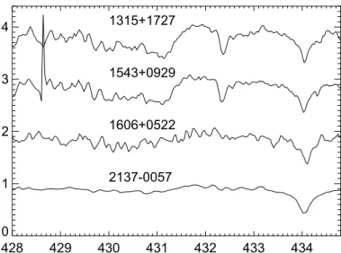
and in Fig.1, we show four of the spectra. We have an

uncer-tainty of 0.15 dex in deriving A(Ca) from the CaII-K line.

The A(Ca) derived from the CaII-K line usually agrees within

uncertainties with the value derived from CaIlines, except for

SDSS J1606+0522, SDSS J0905+0330, and SDSS J1114–1202. For the star SDSS J1606+0522, an uncertainty of 0.31 dex is reasonable because of the spectrum quality, but the scatter of

Fig. 1.Observed spectra for four stars in the range of the G-band.

Fig. 2.Observed spectrum of SDSS J1114–1202 (solid black) compared with a synthetic spectrum (solid red) with A(Ca) compatible with the value derived from the other two CaIlines and with A(Fe).

0.01 dex among the two CaIlines is a random chance event. For

the star SDSS J0905+0330, the A(Ca) is based on the single CaI

line at 422 nm, which is often in disagreement with the other lines. The star is metal poor, therefore a contamination from the

ISM of the CaII-K could increase the A(Ca) derived from this

line. For the star SDSS J1114–1202, the CaII-K line was clearly

too shallow. In Fig.2 we compare the CaII-K line with a

syn-thetic spectrum with a Ca abundance compatible with A(Ca)

derived from two CaI lines and consistent with the Fe

abun-dance. The wings of the CaII-H and -K lines in the synthesis

reproduce the observed spectrum very well, while the core of the line is not present. We suspect that this is due to chromospheric emission. The H-lines in the spectrum of this star are also weak.

In Table2 we also provide a 3D correction on the C

abun-dance as derived from the G-band byGallagher et al.(2016). The

solar A(Fe) used to produce the figures is adopted fromCaffau

et al.(2011), while the other solar abundances are taken from

Lodders et al.(2009).

For two stars, SDSS J1445–0045 and SDSS J0905+0330, we

have hydrodynamical models from the CIFIST grid (Ludwig

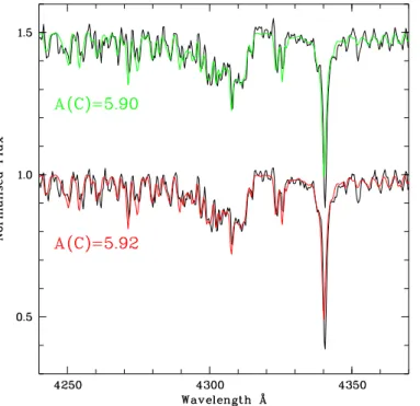
et al. 2009) with parameters very similar to what is observed. We fitted the G bands of these two stars with the synthetic

spec-tra computed using these 3D models withLinfor3D8₍_Gallagher

et al. 2017b). The best fits are presented in Figs.3 and 4. As

8 _{http://www.aip.de/Members/msteffen/linfor3d}

(8)

Fig. 3.Two observed spectra of SDSS J1445–0045 (solid black) com-pared with the best fit (solid green and red) based on a 3D synthesis of a model that is 18 K cooler.

Fig. 4. Observed spectrum of SDSS J0905+0330 (solid black) com-pared with the best fit (solid red) based on a 3D synthesis of a model that is 21 K cooler.

was explained inGallagher et al.(2016), the G-band is extremely sensitive to changes in the oxygen abundance. Because we were unable to directly measure the oxygen abundance, the 3D syn-theses were computed so that oxygen scales with carbon at a consistent ratio corresponding to A(C)–A(O) of –0.67.

4.4. SDSS J1313–0019

In the sample of stars, we also observed SDSS J1313–0019, a star discovered byAllende Prieto et al.(2015) that was later also analysed byFrebel et al.(2015). Both analyses show that the star is an evolved star, extremely low in [Fe/H], with a C content that places the star in the low C band.

The goal of the work presented in this paper is not to improve our knowledge of the chemical composition of this star with the FORS spectra. The aim is instead to test the

Fig. 5.Observed spectrum of SDSS J1313–0010 (solid black) compared with the best fit based on a 3D synthesis with various C/O content. The pink profile corresponds to A(C)–A(O) = –1.67, and the red profile shows A(C)–A(O) = +0.33.

Fig. 6.[Ca/Fe] derived from the CaII-K line vs. [Fe/H]. The black dots surrounded by a red corona represent Ba-rich stars. The solar A(Fe) value of 7.52 is taken fromCaffau et al.(2011), and the solar A(Ca) = 6.33 is adopted fromLodders et al.(2009).

Fig. 7.Carbon abundance vs. [Ca/H] derived from the CaII-K line. The black dots surrounded by a red corona represent Ba-rich stars. An extra green corona is used in the cases of uncertain measurements. Downward arrows represent upper limits.

3D spectra and observationally verify if the C abundance we derive varies by changing the oxygen abundance simulated in the synthesis. The closest 3D model in the CIFIST grid

has parameters Teff= 5500 K, log g of 2.5 [cgs], and [Fe/H]

= −3.0; the model parameters are similar to those suggested by

Allende Prieto et al. (2015) (Te_ff = 5378 K, log g = 3.0,

(9)

Fig. 8.Carbon abundance vs. [Fe/H] of the sample stars (pink and green dots show stars normal and rich in Ba, respectively). Red solid dots are the stars we analysed in the TOPoS project (Bonifacio et al. 2018); the open red dots are taken fromSivarani et al.(2006);Bonifacio et al.(2009,2015);

Spite et al.(2013);Behara et al.(2010);Sivarani et al.(2004) andCaffau et al.(2013a,2016); the black star is taken fromCaffau et al.(2012). The black asterisks show known CH dwarf stars (Karinkuzhi & Goswami 2014,2015). The blue squares show stars from the literature (Yong et al. 2013;

Cohen et al. 2003,2013;Carollo et al. 2014;Masseron et al. 2012;Jonsell et al. 2006;Thompson et al. 2008;Hansen et al. 2015,2016;Lucatello et al. 2003;Aoki et al. 2002,2006,2008;Frebel et al. 2005;Li et al. 2015;Norris et al. 2007;Christlieb et al. 2004;Keller et al. 2014;Frebel et al. 2015;Roederer et al. 2014;Ivans et al. 2005). The blue and orange areas in the figure highlight the two carbon bands as defined inBonifacio et al.

(2018). The black dashed ellipses represent the regions containing the three CEMP populations according toYoon et al.(2016).

[Fe/H] = –4.3, and [C/Fe] = +2.5), with the exception of the iron content. The 3D model was computed with a solar-scaled composition and an enhancement in α-elements of 0.4 dex, typical of a metal-poor star. When computing the synthesis, several C/O ratios were considered. We then fitted the observed profile using a synthesis grid with the same C/O ratio (see

Gallagher et al. 2017a, for details). The fit was also made using

a grid of 1D LHD models (Caffau & Ludwig 2007), computed

with the same C/O ratios. At the typical temperatures, these stars have (5500–6500 K), the A(C) value derived from the 1D fit is not sensitive to changing C/O: a negligible difference of 0.09 dex is found when A(C)–A(O) is varied by up to 2.0. Conversely, the change in the C abundance from the 3D fit is 0.64 dex when A(C)–A(O) is varied by the same amount. When the oxygen abundance is varied for any given carbon abundance, the shape of the G-band varies as well. This is most notable in the band head. However, a higher spectral resolution is required

for this effect to be notable. The fits are shown in Fig.5. The

shape of the G-band also changes by changing C/O; the plot

appears to favour a lower oxygen, and the χ2 test also favours

this case.

5. Results

In Fig.6 we show the [Ca/Fe] versus [Fe/H]. The Ca

abun-dance has been derived from the CaII-K line for this plot, for

which we estimated an uncertainty of 0.15 dex, while the uncer-tainty on Fe is the line-to-line scatter, except for the stars for which no clear Fe line is available; in this case, the uncertainty is related to a comparison with synthetic spectra. The stars, as expected, all seem mostly α-enhanced. The star with the lowest [Ca/Fe] (SDSS J2219+0515) is one with the poorest A(Fe) deter-mination, so that within 1 σ the star is a α-enhanced metal-poor star, at the same level as a typical metal-poor star.

In Fig.7the carbon abundance, derived from the G band and

listed in Table2, is plotted as a function of the [Ca/H] ratio, with

the Ca abundance derived from the CaII-K line. In the figure,

the stars with [Fe/H] < −2 are located in the higher part of the

plot, which means that they belong to the high C band ofSpite

et al.(2013) or have a low A(C) value, placing them on the low

C band. Interestingly, all the stars in the high C band are rich

in Ba (two stars, SDSS J1543+0929 and SDSS J2219+0515, have an uncertain A(Ba) value, which is depicted as a green corona in the figure). The stars belonging to the low C band are not rich in Ba (they have a low [Ba/Fe] or an upper limit): they are CEMP-no stars. Two stars (SDSS J0905+0330 and SDSS J1149+0723) with a very similar A(C) value, just below 7.7, both belong to the higher C band. The latter, SDSS J1149+0723, does not appear to be Ba-rich, but the result, as for the other, is uncertain.

We revisited Fig. 7 by comparing our sample of stars with

the literature in Fig.8. This plot has been devised bySpite et al.

(2013) and was recently revisited by Bonifacio et al. (2018),

who also suggested a classification of CEMP stars according

to C abundance different from the one of Yoon et al. (2016).

The blue and orange areas in the figure highlight the two

car-bon bands as defined inBonifacio et al. (2018), and the three

Yoon groups are delimited by dotted lines. Yoon et al. (2016)

adopted [C/Fe] > 0.7 instead of [C/Fe] > +1.0 for the defini-tion of CEMP stars. Moreover, in their Fig. 1,Yoon et al.(2016) also included giant stars. To define our two regions (orange and blue) in about the same sample of stars, we kept only dwarfs and turn-off stars where the carbon abundance is not affected by mixing. However, at very low metallicity ([Fe/H] < −4.5), we added four giant stars of the low red giant branch, but all with log g > 2.2. For these stars the correction of the carbon abun-dance due to the first dredge-up is small and has been estimated fromBonifacio et al.(2009). As visible in Fig.8, the two regions I and III defined inYoon et al.(2016) are included in our orange and blue areas (as inBonifacio et al. 2018), respectively, while stars in region II are either in our low C band (blue area) or are C-normal, according to our definition. In our interpretation, all C-enhanced stars ([C/Fe] >+1.0 as defined in the introduction)

(10)

Fig. 9.[Sr/Ba] ratio vs. [Ba/Fe]. The black filled circles represent the normal EMP dwarfs and giants studied in the frame of the ESO Large Programme First Stars (Cayrel et al. 2004;Bonifacio et al. 2009) and the stars studied homogeneously bySiqueira-Mello et al.(2015). The black open circles are for CEMP stars studied in the frame of this ESO Large Programme or taken from the literature (Depagne et al. 2002;

Sivarani et al. 2004, 2006;Barbuy et al. 2005; Behara et al. 2010;

Spite et al. 2013;Yong et al. 2013). The green filled squares show nor-mal metal-poor stars studied in this paper, and the open green squares denote the C-rich stars. Note the very peculiar position of the CEMP star SDSS J0222–0313. In this star the first-peak heavy elements (such as Sr) seem to be more enriched than the second-peak heavy elements (like Ba).

in the figure are adequately accounted for by the high and low

C bands (as defined in Bonifacio et al. 2018). The stars

anal-ysed here are shown in Fig.8as pink (normal in Ba) and green

(Ba rich) filled dots, in comparison with other stars taken from the literature. The stars lying below the blue dashed line are carbon-normal stars. In this figure the CEMP ([Fe/H] < −2.0) Ba-rich stars clearly belong to the high C band, while the stars with normal Ba are part of the low C band. The two stars SDSS J0905+0330 and SDSS J1149+0723, one normal and one rich in Ba, but with uncertain measurements, are also similar in [Fe/H] and are placed in the lower part of the high C band or in the upper part of the low C band.

In Fig.9 we compare the position of the most metal-poor

stars in our sample ([Fe/H] < −1.5) with a sample of metal-poor stars collected from the literature, which are, in general, slightly more metal poor than our sample. They are depicted in the form [Sr/Ba] vs. [Ba/Fe]. These stars are generally slightly more metal poor than our sample ([Fe/H] < −2.5). The “normal” stars (i.e. not C-rich) are represented by filled symbols and the C-rich stars ([C/Fe] > 1.0) by open symbols. The green square symbols rep-resent the stars studied in this paper and the black circles show the stars taken from the literature. In normal metal-poor stars, [Sr/Ba] is higher than –0.4, a value observed in particular in the

stars that are strongly enriched in neutron-capture elements, such as CS31082-001, which is explained by a pure r-process enrich-ment and is classified as “r II”. The stars SDSS J2123–0804 and SDSS J0042+0055 could also belong to this class when we take the uncertainties into account.

In Fig.9 several carbon-rich stars are located in the same

region as the “normal” metal-poor stars (CEMP-no). Many CEMP stars are enriched in heavy elements (CEMP-s or -r/s), however, such as in general [Ba/Fe] > 1 and [Sr/Ba] < −0.4; the second peak of the neutron-capture elements such as Ba is more enriched than the first-peak elements such as Sr. SDSS J0222–0313 is characterised by a high value of [Ba/Fe] ([Ba/Fe] = 1.95) and an even higher value of [Sr/Fe] ([Sr/Fe] = 2.25). The high abundance of Sr is also confirmed by the Sr II line at 421.55 nm. In this star the yttrium line (another first-peak neutron-capture element) at 395.04 nm was also detected and measured: [Y/Fe] = +2.57. It would be interesting to be able to measure more neutron-capture elements in this star to explain its unexpected abundance pattern.

6. Conclusions

We analysed 30 unevolved stars and reinvestigated one known

ultra Fe-poor star (Allende Prieto et al. 2015). In spite of the

low resolution of the spectra, we were able to derive very useful information to better understand the C-enhanced stel-lar population. The CEMP stars belonging to the high C band are enhanced in Ba, while those belonging to the low band show a normal A(Ba) value. This finding supports the idea of

Bonifacio et al.(2015) that the high band is populated by binary stars and the high abundances are the result of mass-transfer from a companion, while the stars of the low band, with normal A(Ba), formed from a C-rich gas cloud.

We compared the [Sr/Ba] ratio as a function of [Ba/Fe] for the most Fe-poor stars of this sample to a more metal-poor

sample. In Fig. 9, our stars appear to be similar to the most

metal-poor population; the Ba normal stars are mainly clustered in the upper left side of the diagram and the Ba-rich stars lie in the lower right side. One star, SDSS J0222–0313, is alone in the upper right part of the plot. We need high-resolution observa-tion for this star to confirm with a higher degree of certainty that the first-peak elements (here Sr and Y) are more abundant with respect to Fe than those of the second peak (here Ba).

We also investigated the G-band of the known giant star (Allende Prieto et al. 2015) using a synthesis computed from a hydrodynamical model with parameters similar to those of the star. Because according to the 3D theoretical computation, the shape of the G-band changes as a function of the C/O ratio, we might place constraints on the oxygen abundance by fitting the G-band. In the case of SDSS J1331–0019, a [O/Fe] lower than [C/Fe] is expected. Spectra with a higher resolution would be needed to confirm this, however.

Acnowledgements.This research has made use of the services of the ESO Science Archive Facility. AJG acknowledges the support of the Collaborative Research Centre SFB 881 (Heidelberg University) of the Deutsche Forschungsgemein-schaft (DFG, German Research Foundation). S.D. acknowledges support from Comité Mixto ESO-GOBIERNO DE CHILE.

References

Allende Prieto, C., Fernández-Alvar, E., Aguado, D. S., et al. 2015,A&A, 579, A98

Alvarez, R., & Plez, B., 1998,A&A 330, 1109

Aoki, W., Ryan, S. G., Norris, J. E., et al. 2002,ApJ, 580, 1149

(11)

Aoki, W., Frebel, A., Christlieb, N., et al. 2006,ApJ, 639, 897

Aoki, W., Beers, T. C., Christlieb, N., et al. 2007,ApJ, 655, 492

Aoki, W., Beers, T. C., Sivarani, T., et al. 2008,ApJ, 678, 1351

Appenzeller, I., Fricke, K., Fürtig, W., et al. 1998,The Messenger, 94, 1

Barbuy, B., Cayrel, R., Spite, M., et al. 1997,A&A, 317, L63

Barbuy, B., Spite, M., Spite, F., et al. 2005,A&A, 429, 1031

Beers, T. C., & Christlieb, N. 2005,ARA&A, 43, 531

Beers, T. C., Preston, G. W., & Shectman, S. A. 1985,AJ, 90, 2089

Beers, T. C., Preston, G. W., & Shectman, S. A. 1992,AJ, 103, 1987

Behara, N. T., Bonifacio, P., Ludwig, H.-G., et al. 2010,A&A, 513, A72

Bidelman, W. P. 1956,Vist. Astron., 2, 1428

Bisterzo, S., Gallino, R., Straniero, O., et al. 2006,Mem. Soc. Astron. It., 77, 985

Bonifacio, P., Molaro, P., Beers, T. C., & Vladilo, G. 1998,A&A, 332, 672

Bonifacio, P., Spite, M., Cayrel, R., et al. 2009,A&A, 501, 519

Bonifacio, P., Caffau, E., Spite, M., et al. 2015,A&A, 579, A28

Bonifacio, P., Caffau, E., Spite, M., et al. 2018,A&A, 612, A65

Caffau, E., & Ludwig, H.-G. 2007,A&A, 467, L11

Caffau, E., Ludwig, H.-G., Steffen, M., Freytag, B., & Bonifacio, P. 2011,

Sol. Phys., 268, 255

Caffau, E., Bonifacio, P., François, P., et al. 2012,A&A, 542, A51

Caffau, E., Bonifacio, P., François, P., et al. 2013a,A&A, 560, A15

Caffau, E., Bonifacio, P., Sbordone, L., et al. 2013b,A&A, 560, A71

Caffau, E., Bonifacio, P., Spite, M., et al. 2016,A&A, 595, L6

Carollo, D., Freeman, K., Beers, T. C., et al. 2014,ApJ, 788, 180

Cayrel, R., Depagne, E., Spite, M., et al. 2004,A&A, 416, 1117

Christlieb, N. 2003,Rev. Mod. Astron., 16, 191

Christlieb, N., Gustafsson, B., Korn, A. J., et al. 2004,ApJ, 603, 708

Cohen, J. G., Christlieb, N., Qian, Y.-Z., & Wasserburg, G. J. 2003,ApJ, 588, 1082

Cohen, J. G., Christlieb, N., Thompson, I., et al. 2013,ApJ, 778, 56

Cowan, J. J., & Rose, W. K. 1977,ApJ, 212, 149

Depagne, E., Hill, V., Spite, M., et al. 2002,A&A, 390, 187

Frebel, A., Aoki, W., Christlieb, N., et al. 2005,Nature, 434, 871

Frebel, A., Chiti, A., Ji, A. P., Jacobson, H. R., & Placco, V. M. 2015,ApJ, 810, L27

Gaia Collaboration (Brown, A. G. A., et al.) 2016,A&A, 595, A2

Gallagher, A. J., Caffau, E., Bonifacio, P., et al. 2016,A&A, 593, A48

Gallagher, A. J., Caffau, E., Bonifacio, P., et al. 2017a,A&A, 598, L10

Gallagher, A. J., Steffen, M., Caffau, E., et al. 2017b,Mem. Soc. Astron. It., 88, 82

Gimeno, G., Roth, K., Chiboucas, K., et al. 2016,Proc. SPIE, 9908, 99082S

Gustafsson, B., Edvardsson, B., Eriksson, K., et al. 2008,A&A 486, 951

Hampel, M., Stancliffe, R. J., Lugaro, M., & Meyer, B. S. 2016,ApJ, 831, 171

Hansen, T., Hansen, C. J., Christlieb, N., et al. 2015,ApJ, 807, 173

Hansen, T. T., Andersen, J., Nordström, B., et al. 2016,A&A, 588, A3

Hook, I. M., Jørgensen, I., Allington-Smith, J. R., et al. 2004, PASP, 116, 425

Ivans, I. I., Sneden, C., Gallino, R., Cowan, J. J., & Preston, G. W. 2005,ApJ, 627, L145

Jonsell, K., Barklem, P. S., Gustafsson, B., et al. 2006,A&A, 451, 651

Karinkuzhi, D., & Goswami, A. 2014,MNRAS, 440, 1095

Karinkuzhi, D., & Goswami, A. 2015,MNRAS, 446, 2348

Keller, S. C., Bessell, M. S., Frebel, A., et al. 2014,Nature, 506, 463

Li, H.-N., Zhao, G., Christlieb, N., et al. 2015,ApJ, 798, 110

Lodders, K., Palme, H., & Gail, H.-P. 2009, inLandolt-Börnstein - Group VI Astronomy and Astrophysics Numerical Data and Functional Relationships in Science and Technology, ed. J. E. Trümper, (Berlin: Springer-Verlag), 4B, 560

Lucatello, S., Gratton, R., Cohen, J. G., et al. 2003,AJ, 125, 875

Lucatello, S., Tsangarides, S., Beers, T. C., et al. 2005,ApJ, 625, 825

Ludwig, H.-G., Caffau, E., Steffen, M., et al. 2009,Mem. Soc. Astron. It., 80, 711

Masseron, T., Johnson, J. A., Lucatello, S., et al. 2012,ApJ, 751, 14

McCarthy, M. F. 1994,The MK Process at 50 Years: A Powerful Tool for Astro-physical Insight, eds. C. J. Corbally, R. O. Gray, & R. F. Garrison,ASP Conf. Ser., 60, 224

McClure, R. D. 1984,PASP, 96, 117

McClure, R. D. 1997,PASP, 109, 536

McClure, R. D., & Woodsworth, A. W. 1990,ApJ, 352, 709

McWilliam, A., Preston, G. W., Sneden, C., & Searle, L. 1995,AJ, 109, 2757

Norris, J. E., Ryan, S. G., & Beers, T. C. 1997a,ApJ, 488, 350

Norris, J. E., Ryan, S. G., & Beers, T. C. 1997b,ApJ, 489, L169

Norris, J. E., Christlieb, N., Korn, A. J., et al. 2007,ApJ, 670, 774

Plez, B. 2012,Astrophysics Source Code Library [record ascl: 1205.004]

Roederer, I. U., Preston, G. W., Thompson, I. B., Shectman, S. A., & Sneden, C. 2014,ApJ, 784, 158

Sbordone, L., Caffau, E., Bonifacio, P., & Duffau, S. 2014, A&A, 564, A109

Secchi, A. 1868, Sugli spettri prismatici delle stelle fisse (Roma: Trip. Belle Arti), 11

Siqueira-Mello, C., Andrievsky, S. M., Barbuy, B., et al. 2015, A&A, 584, A86