HAL Id: halshs-02412948
https://halshs.archives-ouvertes.fr/halshs-02412948
Submitted on 16 Dec 2019HAL is a multi-disciplinary open access archive for the deposit and dissemination of sci-entific research documents, whether they are pub-lished or not. The documents may come from teaching and research institutions in France or abroad, or from public or private research centers.
L’archive ouverte pluridisciplinaire HAL, est destinée au dépôt et à la diffusion de documents scientifiques de niveau recherche, publiés ou non, émanant des établissements d’enseignement et de recherche français ou étrangers, des laboratoires publics ou privés.
Towards phonetic interpretability in deep learning
applied to voice comparison
Emmanuel Ferragne, Cédric Gendrot, Thomas Pellegrini
To cite this version:
Emmanuel Ferragne, Cédric Gendrot, Thomas Pellegrini. Towards phonetic interpretability in deep learning applied to voice comparison. ICPhS, Aug 2019, Melbourne, Australia. pp.ISBN 978-0-646-80069-1. �halshs-02412948�
TOWARDS PHONETIC INTERPRETABILITY IN DEEP LEARNING
APPLIED TO VOICE COMPARISON
Emmanuel Ferragne1, Cédric Gendrot1, Thomas Pellegrini2
1Laboratoire de Phonétique et Phonologie (UMR7018, CNRS - Sorbonne Nouvelle) 2Institut de Recherche en Informatique de Toulouse (UMR5505, CNRS - Université de Toulouse)
ABSTRACT
A deep convolutional neural network was trained to classify 45 speakers based on spectrograms of their productions of the French vowel/˜A/. Although the model achieved fairly high accuracy – over 85 % – our primary focus here was phonetic interpretability rather than sheer performance. In order to better un-derstand what kind of representations were learned by the model, i) several versions of the model were trained and tested with low-pass filtered spectro-grams with a varying cut-off frequency and ii) classi-fication was also performed with masked frequency bands. The resulting decline in accuracy was uti-lized to spot relevant frequencies for speaker classi-fication and voice comparison, and to produce pho-netically interpretable visualizations.
Keywords: voice comparison, deep learning, foren-sic phonetics, vowels.
1. INTRODUCTION
Ever since the sound spectrograph was invented in the 1940s [9], phoneticians have mostly relied on vi-sualizations to identify the relevant parameters (for-mants, VOT, etc.) to describe phonetic entities (vow-els, voicing, etc.). The advent of deep learning around 2010 has led to a situation where very power-ful tools are now available to carry out this task auto-matically. A well-known advantage of deep neural networks (DNN) over more conventional machine learning algorithms is that they can extract features from the raw data without the need for a human expert to explicitly provide them to the model [5]. In other words, after 70 years or so of visual iden-tification of acoustic cues to account for phonetic phenomena, DNNs could now potentially take over from human experts. On the downside, DNNs have earned a bad reputation because of their lack of transparency. We would like to show one way to overcome this difficulty with preliminary results we obtained in the field of forensic voice comparison.
In speech processing, DNNs have been success-fully applied to acoustic modelling at phone level for speech recognition [7] and language identifi-cation [10], for instance. In speaker recognition, DNNs were efficient in an indirect manner: instead of being used as classifiers, they were used as feature extractors, with so-called bottleneck features [11] and embeddings [19]. In the current work, we performed speaker identification on a small speech dataset comprised of occurrences of one vowel. Thus, our work is closer to voice comparison rather than speaker identification, which would involve thousands of speakers and longer speech excerpts. DNNs, namely multi-layer perceptrons [13] and convolutional neural networks (CNNs) [16], have been shown to capture high-level phonetic proper-ties when trained as phoneme recognizers. These studies highlighted that neuron units and convolu-tion filters become selective to phonetic features such as manner and place of articulation.
We ran three experiments with a deep CNN and interpreted the output of our models in terms fre-quency bands located in the broadband spectrogram that phoneticians are most familiar with. In the first experiment the model classified 45 speakers based on their production of the French vowel /˜A/. In the second experiment the same model was retrained and tested with low-pass filtered tokens with various cutoff frequencies. In the third experiment, occlu-sion sensitivity was performed: we observed how the masking of certain frequency bands affected the model’s performance. The vowel/˜A/ was used be-cause preliminary trials with other vowels from the same corpus showed that /˜A/ yielded the highest speaker classification rates, which agrees well with the consistent finding in the literature that nasals, and especially nasal vowels [1], tend to contain more speaker-specific information than other segments.
2. SPEECH MATERIAL
The vowels used for classification were extracted from the ESTER Corpus [3], which is a collection of recorded journalistic radio broadcast generally con-sidered as prepared rather than read or spontaneous speech [4]. France Inter, France Info and Radio France International constitute the three sources for our extractions. We used the phonetic alignment provided with the corpus by the IRISA (Institut de Recherche en Informatique et Systèmes Aléatoires) through the AFCP (Association Francophone de la Communication Parlée) website (http://www.afcp-parole.org/camp_eval_systemes_transcription/). Automatic alignment was used to extract vowels with a rectangular window shape and without their phonetic context, the latter being neither controlled nor provided to the network for the discrimination.
3. SPECTROGRAMS
Phoneticians are used to reading broadband spectro-grams. In the Praat program [2], default settings are 5-ms analysis frames and 2-ms hop size. Based on these values, we chose to use 5.0625 ms frames and 0.5 ms hop size to get a 90 % overlap between neigh-boring frames. With a 16 kHz sampling rate, these corresponded to frames of 81 samples. An odd num-ber of samples allows to perform zero-phase win-dowing, which guarantees that the signal portions used to compute the Fast Fourier Transform (FFT) are as symmetric as possible in order to get pure real-valued spectra [18]. The speech segments were element-wise multiplied by a Hamming window and padded to obtain 512-sample segments on which FFT was computed. No pre-emphasis was applied since it increases the amplitude of high frequencies and decreases the amplitude of lower bands and, thus, changes the auditory perception when resyn-thesizing back to time domain. We avoided this artifact because we are planning perceptual exper-iments in the project. Finally, the dynamic range was set to 70 dB to prevent the CNN from identi-fying speakers based on dynamic instead of spec-tral cues. Other values were tested by resynthesizing several signals, and the 70 dB value was the one that least impacted the auditory perception of the speak-ers. Vowels whose duration was greater than 250 ms were left out; the shortest vowels were 30 ms long. Spectrograms of vowels shorter than 250 ms were padded with zeros in order for all spectrograms to have equal width. They were then converted to 8-bit grayscale images and resized to 224 × 224 pix-els, where a pixel was equal to 1.15 ms in the time dimension and 35.71 Hz in terms of frequency.
Con-version to 8 bits was performed so that GPU mem-ory would handle mini-batches of sufficient size for learning to take place.
4. MODEL
We used VGG16 [17], a well-known deep convolu-tional neural network that has become a reference in image recognition. VGG16 and variants called "VGGish" models [6] have been widely used in audio-related tasks for their simplicity and good per-formance, as in [14] for large-scale speaker identifi-cation. In our experiments, the model was re-trained from scratch with randomly initialized weights. All models were trained using an NVIDIA GTX 1080 GPU with the Adam optimizer [8], with a gradient decay factor of 0.900, and a squared gradient decay factor of 0.999. The initial learn rate was 0.0001 and the mini-batches contained 56 spectrograms.
5. EXPERIMENTS
The smallest number of/˜A/ tokens produced by one speaker was 334; so 334 occurrences were randomly picked from the remaining 44 speakers, yielding a final dataset of 15,030 spectrograms. It was ran-domly split into a training, a validation, and a test set containing 10,530 (70 %), 1,485 (10 %), and 3,015 (20 %) tokens, respectively.
5.1. Speaker classification
In this first experiment, speaker classification was carried out. The stopping criterion was reached af-ter 8 epochs. The average accuracy of the model on the test set reached 85.37 % with individual scores ranging from 59.70 to 98.51 %. The mean score was 83.88 % for the 10 women and 85.80 % for the 35 men; the difference between men and women failed to reach statistical significance according to a Mann-Whitney U test (p = 0.32). While such a high clas-sification rate constitutes an interesting finding in it-self, it is quite frustrating for phoneticians because at this stage we have no means of knowing what repre-sentations the model has learned, and the small num-ber of misclassified items does not quite lend itself to fruitful phonetic interpretation. To illustrate this point, among the 990 possible pairwise confusions, 235 contain non zero values; and among them, 194 are constituted of one or two misclassified tokens.
5.2. Low-pass filtered speech
The spectrograms used in Section 5.1 were cropped to obtain seven different versions of the original
dataset with maximal frequencies ranging from 250 to 6,000 Hz. The impact of cutoff frequency on model accuracy is shown in Fig. 1 (the results for the unaltered spectrograms were added for the sake of completeness). Fig. 1 shows a steep increase in accuracy between 250 and 1,000 Hz; then scores rise much more slowly from 1,000 Hz upwards.
Figure 1: CNN accuracy depending on low-pass cutoff frequency (mean and standard deviation).
The lowest accuracy score, 50.85 % obtained with a cut-off frequency of 250 Hz, was significantly above chance (χ2 = 38479 p < 0.001). Mid-p-value McNemar tests were conducted to check if im-provements in accuracy from one model to the next were statistically significant. Each of the models with cut-off frequencies from 500 to 1,000 Hz shows a highly significant improvement over the model with the next lower cut-off frequency. The model with a cut-off at 2,000 Hz shows no significant im-provement compared to the model with a cut-off at 1,000 Hz (p = 0.580). The 3,000 Hz model did not perform better than the 2,000 Hz (p = 0.151) or the 1,000 Hz model (p = 0.074). Then all remaining models improved on the preceding one, although the increased accuracy from 4,000 to 6,000 Hz was only marginally significant (p = 0.012).
A legitimate question here is whether speakers get consistent relative accuracy scores across all cut-off frequencies. In order to test this possibility, for each frequency, speakers were ranked accord-ing to their score and Kendall’s concordance coef-ficient was computed. The outcome was not sta-tistically significant (W = 0.11 χ2 = 43.39 d f = 44 p = 0.50), which supports the view that rela-tive accuracy scores among speakers are inconsis-tent from one frequency step to the next.
5.3. Occlusion sensitivity
The model trained in Section 5.1 was used here. The test phase was different however: test spectrograms were modified by means of a mask (an array of ze-ros) occluding 15 contiguous pixels (≈ 536 Hz) in
the frequency dimension over the whole duration of the vowel. For each vowel, the position of the mask was moved iteratively by one pixel along the verti-cal axis, each time generating a new test image. The initial position of the mask only occluded the lowest pixel row of the spectrogram, and the final position was reached when only the topmost pixel row in the spectrogram was affected. The process yielded 252 new spectrograms for each of the 3,015 (67 test vow-els × 45 speakers) that were classified by the model. At the end of the experiment, the 67 individual test spectrograms were converted to heatmaps where the color of a frequency band reflected the probabil-ity that the vowel belonged to its true speaker class when this frequency band had been occluded. In or-der to determine which frequency bands were typ-ical of a given speaker, the mean and standard de-viation of each speaker’s 67 heatmaps were com-puted, and a signal to noise ratio (SNR) was ob-tained by computing the pixel-wise ratio of the mean heatmap to the standard deviation heatmap for each speaker. The intensity values of the SNR heatmaps were rescaled to the interval ranging from the small-est to the highsmall-est value found in the whole dataset.
Fig. 2 shows two SNR heatmaps. The heatmap in the left panel, showing the output of the occlu-sion technique with the test vowels of Speaker 35, happens to contain the lowest SNR value in our data and therefore exemplifies the darkest shade of blue (slightly above 5 kHz). The picture to the right of Fig. 2 illustrates the highest SNR value (around 1 kHz) in our dataset, which is represented by the darkest type of red in our colormap.
Figure 2: Two SNR heatmaps (kHz).
The salient red stripe shows that when this re-gion in Speaker 45’s spectrograms is hidden from the model, the probability that Speaker 45 is cor-rectly classified drops abruptly and the resulting per-formance deterioration is very consistent across all 67 test spectrograms for this speaker. In contrast, in the left panel of Fig. 2, though critical regions emerged for Speaker 35 (slightly above 1 kHz and between 2 and 3 kHz), they are not as strong as what was found for Speaker 45, hence their green to yel-low color.
5.4. Linking classification, filtering and occlusion
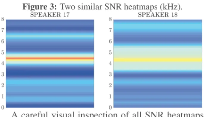
While Speakers 35 and 45 have remarkable SNR heatmaps, containing either the minimal or maxi-mal value computed over all speakers, their results in Section 5.1 and Section 5.2 are not markedly dis-tinct. In the 1st experiment their accuracy scores lie between the 1st and 3rd quartile. Their accu-racy curves in the 2nd experiment exhibit some dif-ferences: Speaker 35 displays a steep accuracy in-crease from 41.79 % (250 Hz) to 94.03 % (3,000 Hz) while Speaker 45’s curve rises more slowly from 64.18 % to 88.06 % over the same frequency inter-val. The link between classification accuracy and what SNR heatmaps show is not straightforward. After computing distances between heatmaps and converting the confusion matrix from experiment 1 to distances, the correlation between the two matri-ces was rather weak: r = 0.187 (though highly sig-nificant: p < 0.001 according to a Mantel test with 100,000 permutations). To what extent the visual similarity between two heatmaps reflects confusabil-ity between two speakers is further exemplified by Fig. 3: the heatmaps look similar and the speakers show confusions in all the models. However, this pair is not the one that exhibits the highest confusion rates; a visual analysis of the two SNR heatmaps is therefore not good indicator of confusability.
Figure 3: Two similar SNR heatmaps (kHz).
A careful visual inspection of all SNR heatmaps suggests that at least 35 of the 45 heatmaps display a relatively strong frequency band around 1 kHz, like both heatmaps in Fig. 2, which points to the impor-tance of this region to characterize a speaker’s voice.
6. DISCUSSION AND CONCLUSION DNNs have often been regarded as blackboxes be-cause of the opaqueness of their inner mechanisms, but efforts have been made in recent years to provide experts in different fields with easily interpretable visualizations of what DNNs learn. Most of these techniques were invented in the context of image recognition and computer vision, and we tried to adapt one of them to spectrograms. As far as we can
tell, the method we used here, inspired by [21], as well as the localization of discriminative regions in [22] or saliency maps in [15] (the latter in the field of audio signal processing) can all be successfully transferred to the study of phonetics.
Our heatmaps constitute data-driven representa-tions of potentially critical spectral regions that are typical of a given speaker’s voice. We devised a method that combines information about how crit-ical a spectral region is and how consistent this re-gion is across several spectrograms of a speaker. A thorough visual analysis of the SNR heatmaps re-veals two important features: first, not all speakers display such critical and reliable frequency bands to the same extent, and second, whenever critical bands are present, they can be found in different regions from one speaker to the next although the 1 kHz re-gion is quite consistently present for most speakers. More research is needed to explore the full poten-tial of our SNR heatmaps especially because, as we have shown, two very similar images do not nec-essarily correlate with high reciprocal confusability. Intuitively, an interesting connection may exist be-tween a heatmap and the concept of distinctiveness in perceptual voice recognition [20], if we go so far as to equate high spectral saliency and low within speaker-variation to distinctiveness.
Spectrograms of the French vowel /˜A/ were fed to a CNN to perform speaker classification based on a corpus of 45 speakers. While accuracy rates were satisfactory, low-pass filtering with varying cut-off frequencies and occlusion sensitivity were used to discover what features the model had learned. A notable finding was that even when the model had very little information (spectral content only up to 250 Hz) it performed well above chance. An-other key finding made possible by our new SNR heatmaps is that many speakers displayed a criti-cal region – a frequency band that, when occluded, led the speaker to be misclassified – around 1 kHz. While SNR heatmaps constitute a promising ap-proach to understanding what DNNs learn, they have yet to be validated with perceptual experi-ments, which is our next logical step in the project. On the epistemological level, we hope that this study exemplifies how the (statistical) acoustic-phonetic and the automatic approaches to forensic voice com-parison [12] can potentially reinforce each other.
7. ACKNOWLEDGEMENTS
This work was supported by the Agence Nationale de la Recherche projects VOXCRIM (ANR-17-CE39-0016) & LUDAU (ANR-18-CE23-0005-01).
8. REFERENCES
[1] Ajili, M., Bonastre, J.-F., Ben Kheder, W., Rossato, S., Kahn, J. Dec. 2016. Phonetic content impact on Forensic Voice Comparison. 2016 IEEE Spoken Language Technology Workshop (SLT)San Diego. IEEE p. 210–217.
[2] Boersma, P. 2001. Praat, a system for doing pho-netics by computer. Glot International 5:9/10, p. 341–345.
[3] Galliano, S., Geoffrois, E., Mostefa, D., Bonastre, J.-F., Gravier, G. 2005. ESTER Phase II Evalua-tion Campaign for the Rich TranscripEvalua-tion of French Broadcast News. Proc. Interspeech Lisboa, Portu-gal. p. 1149–1152.
[4] Gendrot, C., Adda-Decker, M. 2005. Impact of du-ration on F1/F2 formant values of oral vowels: an automatic analysis of large broadcast news corpora in French and German. Proc. Interspeech Lisbon. p. 2453–2456.
[5] Goodfellow, I., Bengio, Y., Courville, A. 2016. Deep Learning. Adaptive computation and ma-chine learning. Cambridge, Massachusetts: The MIT Press.
[6] Hershey, S., Chaudhuri, S., Ellis, D. P. W., Gem-meke, J. F., Jansen, A., Moore, C., Plakal, M., Platt, D., Saurous, R. A., Seybold, B., Slaney, M., Weiss, R., Wilson, K. 2017. CNN architectures for large-scale audio classification. Proc. ICASSP New Or-leans. 131–135.
[7] Hinton, G., Deng, L., Yu, D., Dahl, G. E., Mo-hamed, A.-r., Jaitly, N., Senior, A., Vanhoucke, V., Nguyen, P., Sainath, T. N., others, 2012. Deep neu-ral networks for acoustic modeling in speech recog-nition: The shared views of four research groups. IEEE Signal processing magazine29(6), 82–97. [8] Kingma, D. P., Ba, L. J. 2015. Adam: A Method for
Stochastic Optimization. International Conference on Learning Representations (ICLR). arXiv.org. [9] Koenig, W., Dunn, H. K., Lacy, L. Y. 1946. The
Sound Spectrograph. The Journal of the Acoustical Society of America18(1), p. 19–49.
[10] Lozano-Diez, A., Plchot, O., Matejka, P., Gonzalez-Rodriguez, J. 2018. DNN based embed-dings for language recognition. Proc. of ICASSP Calgary. p. 5184–5188.
[11] Matˇejka, P., Glembek, O., Novotn`y, O., Plchot, O., Grézl, F., Burget, L., Cernock`y, J. H. 2016. Anal-ysis of dnn approaches to speaker identification. Proc. ICASSP. IEEE p. 5100–5104.
[12] Morrison, G. S., Thompson, W., C. 2017. Assess-ing the admissibility of a new generation of foren-sic voice comparison testimony. Columbia Science and Technology Law Review18, p. 326–434. [13] Nagamine, T., Seltzer, M. L., Mesgarani, N. 2015.
Exploring how deep neural networks form phone-mic categories. Proc. Interspeech Dresden. p. 1912–1916.
[14] Nagrani, A., Chung, J. S., Zisserman, A. 2017. Voxceleb: a large-scale speaker identification dataset. Proc. Interspeech Stockholm.
[15] Pellegrini, T. 2017. Densely connected CNNs for bird audio detection. Proc. EUSIPCO Kos. p. 1784–88.
[16] Pellegrini, T., Mouysset, S. 2016. Inferring phone-mic classes from CNN activation maps using clus-tering techniques. Proc. Interspeech San Franscico. p. 1290–1294.
[17] Simonyan, K., Zisserman, A. 2015. Very Deep Convolutional Networks for Large-Scale Image Recognition. ICLR 2015 San Diego.
[18] Smith, J. O. accessed 13/11/2018. Spectral audio signal processing. http://ccrma.stanford.edu/~jos/ sasp/. online book, 2011 edition.
[19] Snyder, D., Garcia-Romero, D., Povey, D., Khu-danpur, S. 2017. Deep neural network embeddings for text-independent speaker verification. Proc. In-terspeechStockholm. p. 999–1003.
[20] Stevenage, S. V. July 2018. Drawing a distinction between familiar and unfamiliar voice processing: A review of neuropsychological, clinical and em-pirical findings. Neuropsychologia 116, 162–178. [21] Zeiler, M. D., Fergus, R. 2014. Visualizing and
un-derstanding convolutional networks. In: Fleet, D., Pajdla, T., Schiele, B., Tuytelaars, T., (eds), Com-puter Vision – ECCV 2014volume 8689. Springer p. 818–833.
[22] Zhou, B., Khosla, A., Lapedriza, A., Oliva, A., Tor-ralba, A. June 2016. Learning deep features for dis-criminative localization. 2016 IEEE Conference on Computer Vision and Pattern Recognition (CVPR) Las Vegas. IEEE p. 2921–2929.