Experimental procedures for determination of dynamic response using system identification techniques

Publisher’s version / Version de l'éditeur:

Journal of Thermal Insulation, 11, pp. 120-43, 1987-10

READ THESE TERMS AND CONDITIONS CAREFULLY BEFORE USING THIS WEBSITE. https://nrc-publications.canada.ca/eng/copyright

Vous avez des questions? Nous pouvons vous aider. Pour communiquer directement avec un auteur, consultez la première page de la revue dans laquelle son article a été publié afin de trouver ses coordonnées. Si vous n’arrivez pas à les repérer, communiquez avec nous à PublicationsArchive-ArchivesPublications@nrc-cnrc.gc.ca.

Questions? Contact the NRC Publications Archive team at

PublicationsArchive-ArchivesPublications@nrc-cnrc.gc.ca. If you wish to email the authors directly, please see the first page of the publication for their contact information.

NRC Publications Archive

Archives des publications du CNRC

This publication could be one of several versions: author’s original, accepted manuscript or the publisher’s version. / La version de cette publication peut être l’une des suivantes : la version prépublication de l’auteur, la version acceptée du manuscrit ou la version de l’éditeur.

Access and use of this website and the material on it are subject to the Terms and Conditions set forth at

Experimental procedures for determination of dynamic response using

system identification techniques

Haghighat, F.; Sander, D. M.

https://publications-cnrc.canada.ca/fra/droits

L’accès à ce site Web et l’utilisation de son contenu sont assujettis aux conditions présentées dans le site LISEZ CES CONDITIONS ATTENTIVEMENT AVANT D’UTILISER CE SITE WEB.

NRC Publications Record / Notice d'Archives des publications de CNRC:

https://nrc-publications.canada.ca/eng/view/object/?id=54c3ddeb-4414-4937-a3b4-13152aca7c3e https://publications-cnrc.canada.ca/fra/voir/objet/?id=54c3ddeb-4414-4937-a3b4-13152aca7c3e

Ser

National Research Conedl national

TH1

b l

_{CouncII Canada d .Canada ~ ~}

N21d

no.

1567

_{Institute for lnstitut de}

c. 2 Research in recherche en

BLDG

'

_{Construction construction}

Experimental Procedures for

Determination

of

Dynamic

Response

Using

System

Identification Techniques

by F. Haghighat and D.M. Sander

Reprinted from

Journal of Thermal Insulation Vol. 11

-

October 1987 p. 120- 143

(IRC Paper No. 1567)

NRC

-

CISTI

h

I R C

L I B R A R Y

I NRCC 29651

Les auteurs examinent des m6thodes servant B determiner la rkponse thermique dynamique

B

l'aide de techniques d'identification de systknes. 11s dhivent un essai utilisant en en&e une sCquence multifi6quence binaire pour dCterminer la dponse d'un CchantilIon de mat&au

.

11s obtiennent les coefficients de fonction de transfert z au moyen du calcul de la rdponse de fm5quence et de la dgression par la methode des moindres carr6s en domaine de temps.

Experimental Procedures for

Determination of Dynamic Response

Using System Identification Techniques

F.

HAGHIGHAT

Centerfor Building Studies Concordia University

Montreal, Quebec H3C 1M8 Canada

D.

M. SANDER

National Research Council Canada Institute for Research in Construction Ottawa, Ontario, Canada KIA O R 6

ABSTRACT

Methods for determining dynamic thermal response using systems identification techniques are discussed. A test using a binary multi-frequency sequence as input to determine the response of a material sample is described. Z-transfer function coeffi- cients are obtained using both frequency response analysis and least squares regres- sion in time domain.

INTRODUCTION

K

NOWLEDGE O F THE dynamic response of building envelope com- ponents is important in the design of thermal systems. The load cal- culation method given in the ASHRAE Handbook [I] is based on the "z- transfer function" method developed by Stephenson and Mitalas [2]. The coefficients for walls and roofs are obtained either from tables contained in the Handbook or by means of a computer program [3]. In either case, these coefficients are derived from an analytical method which assumes that the construction consists of layers of homogenous material and that heat flow is

Detewnining Dynamic Thermal Response 121

one-dimensional. In practice, actual walls contain heat bridges, such as studs or structural members, and may be composed of non-homogenous materi- als. Furthermore, the properties of the materials may be unknown or diffi- cult to determine. Therefore, there is a need for experimental methods to de- termine the dynamic thermal performance of components.

This paper discusses some of the procedures for determining dynamic re- sponse, and describes a test on a slab of homogeneous material to demon- strate one of these techniques.

A complete dynamic model for heat flow through a component is com- monly represented in the matrix notation introduced by Pipes [4] which relates the temperatures and heat flows at both surfaces (see Figure 1).

The transfer function of interest for load calculations is

-

lIB, which re-

lates the heat flow at the inside surface, Q2, to the temperature at the outside

surface,

el,

with the boundary condition of a constant inside temperature,

0 2 .

In z-transfer hnction form this is written as

This transfer function is used to simulate the response by calculating heat

flux Q, a t time r from a history of v~lucs t;)r (J2 J I I ~ t),.

where A is the time interval for thc sin~ulation

SYSTEM IDENTlFICATlON

The use of system identification methods to dctcrminc pararilctcrs oi a

system is well established [5,6]. Thcsc arc methods of obtaining a mathe- matical model for a system on the basis of analysis of input and output sig- nals. This requires both selection of the form of the model (i.c.. the equation) and estimation of values for the parameters in the model. The existence of many different solutions for a given system is common. Thcrc is generally a compromise between modelling error and complexity. Therefore, thc selcc- tion of the model depends upon the purpose of the identification and the ex- perience of the user. While system identification techniques may employ non-linear models, the techniques described in this paper are applicable only when linearity can be assumed. Both the z-transfer function and the Fourier transform are valid only for linear systems. Heat transfer problems are nor- mally considered linear, but t h s may be inappropriate in some cases such as when heat transfer is primarily by radiation or when moisture is present in a porous material.

Various input signals may be employed. A step input is the simplest for the purpose of system identification. This signal provides a good insight into the transient response of the system. For a first-order system the steady state gain and time constant may easily be determined. Methods also exist [7] to identify higher order systems. Similarly, the parameters of a system can be obtained using a ramp input signal [8], since a ramp is the integral of a step function. For a linear system, the relationshp between the input, ~ ( t ) , and the output, y ( t ) , is given by the convolution integral

y ( t ) =

S

h(u)x(t - u)du (5) where h(u), the weighting function, describes the dynamic characteristics of the system. Therefore, theoretically, a unit impulse would be the ideal input signal since the resulting output would be the weighting function h (u). (The weighting function is essentially the same as the response factors referred to by Mitalas [9].) However, in practice it is impossible to produce a true im-

Determining Dynamic T h e m a l Response 123

pulse and difficult to achieve an approximation which has sufficient magni- tude to yield a usable output.

Frequency response analysis is a classical technique in control engineering and may be used for identification of systems. In its basic form, a sinusoidal input is applied to the system. The system response, at this frequency, can be described by the ratio of amplitude of output to input and the difference in phase between output and input. Repeating for several frequencies provides enough information to plot the amplitude ratio and phase lag versus fre- quency to indicate the system frequency response. The disadvantages of this procedure are that it may be difficult to produce a sinusoidal signal and a series of tests takes a long time. -

These disadvantages may be overcome by Fourier analysis techniques. A periodic signal containing many frequency components is applied to the in- put. A Fourier transform is then performed on both input and output; the result is sufficient information to produce a Bode plot from a single test.

Equation (5) can be transformed to frequency domain as

where

Y(w)

-

Fourier transform of output, y(t) X(w)

-

Fourier transform of input, x(t)

H(w)

-

transfer function, Fourier transform of h(u)

Therefore, H(w) can be obtained from Equation (6), and an inverse Fourier transform of H(w) will yield the describing function h (u).

A convenient type of input signal for Fourier analysis is a binary periodic

sequence [lo]. This signal is easy to generate by simply switching between two states (onloff); it does not require any complex control or waveform generator. Pseudo-random binary signals are often used when frequency re- sponse at many points over a wide frequency range is required. Other forms of binary multi-frequency signal (BMFS) have the characteristic that their power is concentrated in a limited number of frequencies. While this signal gives response information for fewer points over a smaller frequency band- width, it has the advantage that the amplitude of those frequency compo- nents is larger and less susceptible to noise. This type of signal is well suited to response evaluation of systems that have non-resonance or non-rejection response characteristics and was, for this reason, used in the experimental procedure to be described in the following section.

Least squares techniques have also been employed to fit parameter values to a chosen transfer function model in time domain [Ill. These attempts

have encountered difficulty in fitting directly to the z-transfer coefficients of Equation (4). Pedersen and Mouen [12] found the direct solution produced meaningless response factors and chose instead to estimate values of equiva- lent thermophysical properties (conductivity, density and specific heat) us- ing a stochastic gradient algorithm. Sherman et al. [13] defined a set of simplified thermal parameters and used them to characterize the thermal performance of the wall from an arbitrary temperature history using digital filter design.

DESCRIPTION OF TEST APPARATUS AND PROCEDURE

An experiment was performed at the Thermal Insulation Laboratory of the Institute for Research in Construction, National Research Council Can- ada, to investigate test procedures for determining the dynamic heat transfer characteristics of a slab of material. The sample chosen was a sheet of rubber material for whlch the thermal properties (see Appendix A) were known.

The requirements for determination of H are to:

introduce a variation in e l , the temperature on surface 1 measure Q2, the heat flux at surface 2

maintain constant e l , the temperature of surface 2

The simple heat flow meter configuration shown in Figure 2, using a heat flux transducer to measure Q2, is not satisfactory. The problem is that a tem- perature drop, proportional to Q2, appears across the heat flux transducer.

FIGURE 2. Heat flow meter apparatus.

i

s

7

hot piate cold plate

-*

c , ₇

-

-

b

heat flux transducer

-. .

-

-

.-

-

-

-

Determining Dynamic Thermal Response cold plate / (sink)

I

Heater A] - -

i

Heater A2 I I Heater.

FIGURE 3. Schematic of test apparatus.

Therefore, temperature O2 varies, even though the cold plate temperature €3, is kept constant. (An additional difficulty is that the frequency response of the heat flux transducer must be broad enough to cover the frequencies of the test.)

A modification of the 600 rnm heat flow apparatus [14], shown in Figure 3, was used. Temperature

e2

is maintained constant by an electric heater and temperature controller. This heater consists of a metering area surrounded by a guard area, as shown in Figure 4. The guard area is maintained at the same temperature as the metered area to prevent edge losses. The power in- put, P, to the metering area is measured. Because of symmetry, if the tem- perature O2 is maintained perfectly constant the heat flux at the surface is

where A is the metered area.

Temperature €3, was varied by switching heaters A, and A2 on and off. The cold plates were kept at a constant temperature to serve as a sink for the heat ,

Guard Area Meter Area

\ t

FIGURE 4. Schematic of measurement apparatus.

from the heaters. A computer data acquisition system recorded data every 15 seconds.

RESULTS

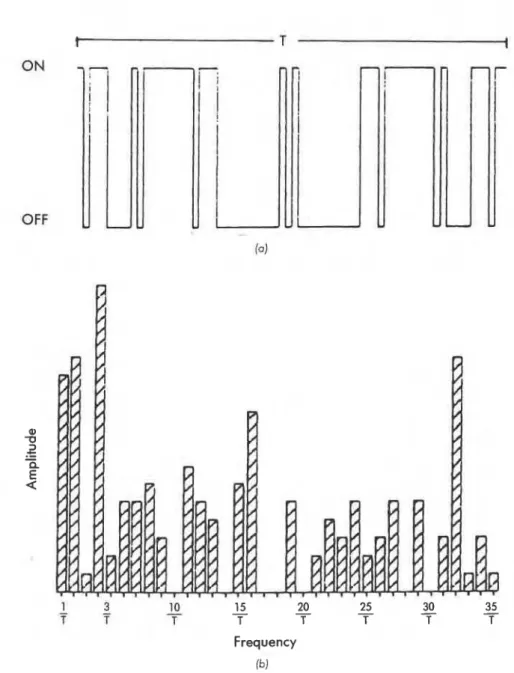
A binary multi-frequency sequence, shown in Figure 5(a), was used as the signal to control the heaters A, and Al. This signal was obtained from the following equation, where the heaters are on when g ( t ) 1 0 and off when

s(t>

s

0.

g ( t ) = cos (o)

-

cos (2w)

+

cos (4w)

-

cos (8o)

+

cos (16w)

-

cos (320)

+

cos (64w) where

and T = period of the sequence. Figure 5(b) shows the amplitude of the fre- quency spectrum of this signal.

Frequency

fb)

FIGURE 5. (a) A multifrequency binary sequence signal with period T; (b) amplitude of fre- quency components of the signal.

Minuter (01 210

-

200

-

190

-

180

-

170

-

160

-

70

-

0 5 10 15 20 25 30 35 40 45 50 55 60 65 70 Minutes (b)

25 20 A m P 15 1 I t u 10 d e 5 0 0.0001 0.001 0.01 Frequency (!/see1 (b)

FIGURE 7. (a) Amplitude of frequencies in the input signal, 19, (degrees C); (b) amplitude frequencies in the output signal, Q2 (wlm").

The resulting temperature

el

and heat flow Ql, after a periodic condition had been established (after 6 periods), are sliown in Figure 6. Figure 7 shows the results of Fourier analysis using a fast Fourier transform [15,16].

The transfer function H(w) was obtained from Equation (6). To reduce the effect of noise, only frequencies at which el(w) had a reasonably large ampli- tude (greater than 0.1) were considered; 14 frequencies met this criterion.

Measured vr Calculated Response

0 -50 -100 1 9 a -if10

-m

-250 0.0001 0.001 0.01 Frequency lilsecl

FIGURE 8. Frequency response obtained from test measurements; theoretical calculated re- sponse shown for comparison.

Determining Dynamic Thermal Response 131 The resulting transfer function, normalized to U-value, is shown in Figure 8. For comparison, the theoretically derived frequency response for the slab of rubber material is also shown.

The agreement between the theoretical and experimental response is good. However, the experimental values show a slight resonance characteristic which would not be associated with the heat transfer process; the amplitude ratio at the first harmonic is slightly greaser than at steady state. Further in- vestigation revealed that the temperature controller was not maintaining

temperature €lZ constant. The frequencies of this variation in were those

displaying the resonance phenomena. The apparent resonance is therefore

attributed to error introduced by variation of the temperature o f mass of the

heater. This highlights the importance of good control when using this ap- proach to measuring heat flow.

Although the frequency response function H ( w ) is very useful, the r - transfer function form is required for load calculations or time-domain ther-

mal simulation. A regression technique can be applied directly to the mea-

sured frequency response data, to fit coefficients to a transfer function of the

form given in Equation (4). In addition to one equation for steady state, two

equations can be written far each frequency: one for the real component and

one for the imaginary component (see Appendix B).

-- - -- - - - - - -

Therefore, for 14 measured frequencies,29 equations can be wGtte<and

regression used to solve for the coefficients. Table 1 gives the coefficients ob-

tained for different numbers of terms in the numerator and denominator.

Higher orders than those shown in Table 1 resulted in unstable simulations. Figure 9 shows the frequency response plots for these derived z-transfer functions. Table 3 gives the response of the z-transfer functions compared to the measured response.

I

2-tnnsitr functlon response

Frequency l i / w c l 0 50 -100

R

I -150 a 8 -200 -250 -300 o . o w 1 0.001 0.01 Frequency I l h s c l

FIGURE 9. Frequency response o f z-transfer functions. Coefficients, obtained from test, are given in Table 1.

regression vs frequency analysls C3,o-31 frequency (ilsecj 0 50

;

-"

8 I e

-m

-200 -250 0.0001 0,OOt 0 Frequency li18ecl

FIGURE 10. Frequency response of z-transfer functions; coefficients (n = 3, rn = 3) obtained from frequency analysis and from time series regression. (See Tables 1 and 2.)

134 F. HAGHIGHAT AND D. M. SANDER

Table 2. Z-transfer function coefficients from regression analysis (A = 60 sec).

Multiple linear regression was also applied directly to the time domain data by fitting coefficients to Equation (4). The resulting coefficients are given in Table 2, and the frequency response shown in Figure 10.

The results were better than expected, since both the authors had experi- enced difficulty with direct fitting of ZTF coefficients to data obtained using pulse or step signals as input. This is probably due to the much better fre- quency distribution of the BMFS excitation. To examine the susceptibility of the analysis to noisy data the input and output were corrupted by rounding to the nearest degree K and nearest 15 wattslm2 respectively. Both time do- main and frequency domain analysis on this "imprecise" data were stable. The results are given in Appendix C.

SUMMARY A N D CONCLUSIONS

In general, the determination of dynamic response involves the following steps: select the form of the model; devise a test apparatus capable of main- taining the boundary conditions and measuring input and output variables; excite with an input signal; fit the model parameters to the measured data. The application of system identification techniques was demonstrated by the experimental determination of dynamic thermal response characteristics of a small homogenous sample. The form of the model was predetermined to be the z-transfer function expressed as a ratio of polynomials [Equation

(3)]. An experiment was devised to maintain the boundary condition of con- stant

el

while values of Q2 and 8, were measured.

A binary multi-frequency sequence (BMFS) was chosen as the input exci- tation for 8,. This type of signal has several attractive characteristics for sys-

I tem identification. It is easy to produce, requiring no complex waveform

generator or precise control. It minimizes the disturbance to the system

I

under test; the mean temperature for the sample tested varied by less than 5OC. It is efficient at concentrating power at appropriate frequencies; a step

I _{input has its energy concentrated at low frequencies, while a pulse contains}

the entire spectrum but at very low amplitudes. The BMFS, in combination with Fourier analysis, takes much less time than testing with an equivalent number of sinusoidal inputs.

Two methods were used to fit ZTF coefficients to the data. conventional multi-linear regression in time domain gave good results, despite the fact

9 @ ? 7 9 7 " ? ? h h 7 " " 9 ? 0 O Q b - O O O O W Q a W O Q - C V O W h W b W N O V W b O I I I I I I I - - - c " I I I I I I I

q

0 0 a W 0 m V h - V w W V 0 0 d & d d C j + d G ~ ~ d L + + , ' j u, - ~ V W I \ W ~ - ~ O W W O - 0 I I I I I I 1 - - - J m

3

I I I I I I I

20 40 Minutes

FIGURE 11.

that previous experience with other forms of input signal had shown prob- lems. This might be attributed to the much better frequency distribution characteristics of the BMFS.

An alternative method of fitting ZTF coefficients is to first obtain the response of the system at a number of frequencies using Fourier analysis, and then use linear regression to fit coefficients to the frequency response data. This technique gives a much better picture of how the system responds at different frequencies. Anomalies in the test results are much more apparent when examining frequency response since the general form of the Bode plot is known. This technique should be less susceptible to noise, and also per- mits the sampling interval for the z-transform to be different from that of the data in the test.

Each of these methods can g v e a number of different sets of coefficients, which are a good representation of the dynamic response; they tend to differ only at the higher frequencies.

The experiment indicated that regression in both time domain and fre- quency domain was robust when applied to data from the BMFS excitation, This was tested by decreasing the resolution of input and output signals to 1 OC and 15 watt/m2 respectively. Analysis of this "imprecise" data yielded the transfer functions shown in Appendix C.

Determining Dynamic Thermal Response 137

The laboratory demonstration on a small homogenous sample indicates that testing using BMFS and frequency analysis has promise for determining dynamic thermal response. This technique is currently being extended, at Concordia University, to larger scale testing on samples of more typical wall construction. By devising a test apparatus with appropriate boundary con- ditions one could apply it to determination of the other functions in the transmission matrix of Equation (1). Since this type of testing has long been used in process industries it could be well suited to determining the dynamic characteristics of other elements, such as HVAC system components, pro- viding these satisfy the restriction that the systems can be considered linear.

ACKNOWLEDGEMENTS

The work described in this paper was carried out at the Institute for Research in Construction at National Research Council Canada with finan- cial support from the Natural Sciences and Engineering Research Council. The authors are grateful for the advice and assistance of their colleagues at IRCINRCC, and especially to R. G. Marchand of the Thermal Insulation Laboratory for making the measurements.

APPENDIX A Description o f Sample

The test sample is a rubber material. The following properties were determined by laboratory measurement:

Density (Q) = 1252.1 kglm3

Specific heat (C,) = 1073.5 JIkgK

Thermal conductivity (A) = 0.2314 WlmK

Thickness (P) = 0.0123 m

The transfer function

QJe,,

in Laplace transform notation, is (from Reference 4)

i

H(s) = Adz

Sinh

(Pm)

where a = XI(C,e) is the thermal diffusivity.

APPENDIX B Derivation of Z-Transfer Function Coefficients from Frequency Response Data

The form o f the z-transfer function is

where

a,...a., bl...b, = coefficients

z-i

-

-

operator representing a time delay = i A where A is the time interval for cal-

culation.

Since z = eA', Equation ( B l ) in Laplace notation becomes

Substituting jw for s,

or, since e-jwA = cos wA-j sin wA,

a,

+

a,[cos (wA) - j sin (wA)]

+

a,[cos (2wA)

-

j sin (2wA)l

+

...

H,,) =

1

+

b,[cos (wA)

-

j sin (oA)]

+

b2[cos (2wA)

-

j sin (2wA)l

+

...

(B4)

...

+

a.[cos ( n o A )

-

j sin (noA)]

... + b,[cos (m wA)

-

j sin (mwA)]

H i s a complex value consisting of a real part H R and an imaginary part HI. Equat-

ing the real and imaginary parts o f Equation (B4) yields

H,,,, = a,

+

a, cos (oA)

+

a, cos (2wA)

+ ...

a. cos (nwA)

-

bl[HR(,) cos (wA)

+

Hdw) sin (wA)]

-

... _(B5)

-

b,[H,,,, cos (m wA)

+

H

,,,,

sin (mwA)]

HI,,) = -a, sin (wA)

-

a, sin (2wA)

-

... - a, sin ( n o A )

+

bl[HR(,) sin (wA)

-

HI(,) cos (oA)]

+

... (B6)

Determining Dynamic Thermal Response 139

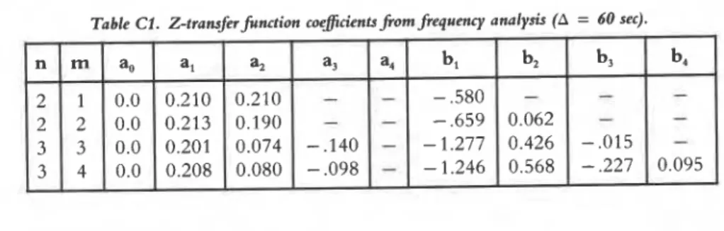
Table C1. Z-transferfunction coeficient~J;om frequency analysis (A = 60 sec).

The Equations (B5) and (B6) can be written for each frequency for which response data is available. In addition, for the steady state condition (w = 0) Equation (B3) reduces to

where U is the steady state U-value.

Thus, if response data for N frequencies is available then 2A'

+

f equations result;

these can easily be solved for the coefficients (ao to a, and 6, to b,) using multiple lin-

ear regression provided the number of coefficients (n

+

m

+

I) is less than the num- ber of equations. Equation (B7) can be given w t m weight to ensure that the z -

transfer function has the correct steady state U-value.

A complication may arise when phase lags of 180' occur. Under this condition the regress~on may produce negative values for ao. This can be prevented by forcing a, to zero in Equations (B5) and (B7).

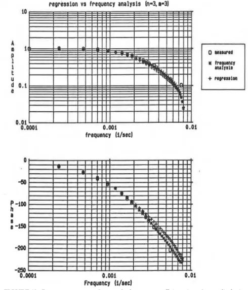
APPENDIX C Analysis Using Imprecise Data

Experience has shown that regrcssion techniques often work well with very prc- cise data, but fail when noise is present in the data. To examine the robustness o f the techniques employed in this paper the data was made less precise by rounding the in- put (temperature difference) to the nearest degree Kelvin and the output (heat flow) to the nearest watt, which corresponds to approximately 15 wlm" This represents approximately a hundredfold reduction in measured precision.

Frequency response analysis was then carried out on this "corrupted" data. The re- sponse obtained is shown in Figure C1. While there is obviously some loss of infor- mation due to the reduced precision the frequency response obtained does not differ

0 p -iW

n

1 S g - 1 9 -250 0.oool 0.001 0.01 Frequency Il/aecl

FIGURE C1. Frequency response obtained from test data made imprecise through rounding to nearest degree and nearest 15 w/m2 (approximately 100 times less precision than actual measurement).

Frequency ll/secl

o.ooa1 0.001

Frequency ll/secl

FIGURE C2. Frequency response of z-transfer functions obtained by fitting to frequency analysis of irn- precise data. Coefficients are given in Table C1.

F. HAGHIGHAT AND D. M. SANDER regress lon vs frequency ant lyslr h-3, r 3 l

FIGURE C3. Frequency response o f 2-transfer functions (11 = 3.1~1 = 3) obtained from frequency analysis

and from time series regression o f imprecise data. (See Tables CI and CZ for coeficicnts.)

greatly from that obtained from the precise mcasuremcnt. Z-transfer function c ~ e f i - cients obtained by fitting to this frequency response are given in Table C1. All o f these produced stable simulations. Figure C2 shows the frequency response o f the Z -

transfer functions.

Regression analysis was also carricd out o n the imprecise data. The resulting z - transfer function coefficients, given in Table C2, give a stable simulation. However, as shown in Figure C3, the frequency response of the z-transfer function from regression is somewhat distorted at high frequencies.

Determining Dynamic Thermal Response 143

I

REFERENCES

1. ASHRAE Handbook of Fundamentals.

2. Stephenson, D. G. and G. P. Mitalas. "Calculation of Heat Conduction Transfer Function for Multi-Layer Slabs," A S H R A E Transactions, V. 77, Part I1 (1971). 3. Mitalas, G. P. and J. G. Arseneault. "Fortran IV Program to Calculate Z-Transfer

Functions for the Calculation of Transient Heat Transfer Through Walls and Roofs," National Research Council Canada, Division of Building Research, C P 33 (1972).

4. Pipes, L. A. "Matrix Analysis of Heat Transfer Problems," Franklin Institute Jour-

nal, 263(3):195-205 (1957).

5. Astrom, K. J. and P. Eykhoff. "System Identification-A Survey," Automatics, 7(2):123-162 (1971).

6. Bekey, G. A. "System Identification-An Introduction and a Survey," Simulation, 15(4):151-166 (1970).

7. Sinha, N. K. and B. Kuszta. Modelling and Identification of Dynamic Systems. Van Nostrand Reinhold Company (1983).

8. Nagrath, I. J. and M. Gopal. Control System Engineering. 2nd edition. Halsted Press (1982).

9. Mitalas, G. P. "Calculation of Transient Heat Flow Through Walls and Roofs,"

A S H R A E Transactions, V. 74, Part I1 (1968).

10. Van den Bos, A. "Construction of Binary Multi-Frequency Signals," IFAC Symp. (1967).

11. Grawford, R. R. and J. E. Woods. "A Method for Deriving a Dynamic System Model from Actual Building Performance Data," A S H R A E Transactions, V. 91, Part 2 (1985).

12. Pedersen, C. 0. and E. D. Mouen. "Application of System IdentificationTeck niques to the Determination of Thermal Response Factors from Experimental Data," A S H R A E Transactions, V. 79, Part 2, pp. 127-136 (1973).

13. Sherman, M. H., R. E. Sonderegger and J. W. Adams. 'The Determination of the Dynamic Performance of Walls," A S H R A E Transactions, V. 88, Part 1 (1982). 14. Bomberg, M. and K. R. Solvason. "Comments on Calibration and Design of a Heat Flow Meter," Thermal Insulation, Materials, and Systems for Energy Con- servation in the 'SOs, ASTM STP 789, American Society for Testing and Materi- als, pp. 277-292 (1983).

15. Bergland, G. S. "A Guided Tour of the Fast Fourier Transform," IEEE Spectrum, pp. 41-52 (July, 1969).

T h i s p a p e r is b e i n g d i s t r i b u t e d i n r e p r i n t form by t h e I n s t i t u t e f o r R e s e a r c h i n C o n s t r u c t i o n . A l i s t o f b u i l d i n g p r a c t i c e a n d r e s e a r c h p u b l i c a t i o n s a v a i l a b l e from t h e I n s t i r u t e may be o b t a i n e d by w r i t i n g t o t h e P u b l i c a t i o n s S e c t i o n , I n s t i t u t e f o r R e s e a r c h i n C o n s t r u c t i o n , N a t i o n a l R e s e a r c h C o u n c i l o f C a n a d a , O t t a w a , O n t a r i o ,

KIA

0R6. Ce document e r t d i s t r i b u 6 s o u s forme d e t i r 6 - 3 - p a r t p a r l l I n s t i t u t de r e c h e r c h e e n c o n s t r u c t i o n . On p e u t o b t a n i r line l i s t e d e s p u b l i c a t i o n s de l l Z n s t i t u t p c r t a n t s u r les t e c h n i q u e s ou Les r e c h e r c h e s e n 1nati0re d e b l t i m e n t e n d c r i v a n t B l a S e c t i o n d e s p u b l i c a t i o n s , I n s t i t u t de r e c h e r c h e e n

c o n s t r u c t i o n , C o n s e i l n a t i o n a l d e r e c h e r c h e s du Canada, Ottawa ( O n t a r i o ) ,