Closed-loop system identification of cardiovascular control mechanisms in diabetic autonomic neuropathy

(1)

Closed-Loop System Identification of

Cardiovascular Control Mechanisms in

Diabetic Autonomic Neuropathy

by

Ramakrishna Mukkamala

Bachelor of Science in Engineering Biomedical and Electrical Engineering

Duke University (1993)

Submitted to the Department of Electrical Engineering and Computer Science in partial fulfillment of the requirements for the degree of

Master of Science at the

Massachusetts Institute of Technology May, 1995

(c) Ramakrishna Mukkamala, 1995

The author hereby grants MIT permission to reproduce and to distribute copies of this thesis document in whole or in part.

Signature of Author ..

Department of Electrical Engineering and Computer Science May 26, 1995 Certified by -... ..-- V ... Richard J. Cohen Thesis Supervisor ~fl-V~L Accepted by

MAS HU8Accepted Erederic by R. Morgenthaler O rTECH.ntt•p par erL Committee on Graduate Studies

JUL 1 71995

I W-S4 I -~IIW_ ~1_1 •:/,"· .

) .. A. I

(2)

Closed-Loop System Identification of Cardiovascular Control Mechanisms in Diabetic Autonomic Neuropathy

by

Ramakrishna Mukkamala

Submitted to the Department of Electrical Engineering and Computer Science on May 26, 1995, in partial fulfillment of the requirements for the degree of

Master of Science

Abstract

The primary focus of this thesis is on the presentation of a sensitive, quantitative method that requires minimal subject cooperation for the assessment of the autonomic nerve damage frequently associated with diabetes mellitus. The method employs a system identification procedure to estimate the open-loop couplings between the beat-to-beat fluctuations in heart rate, arterial blood pressure, and instantaneous lung volume described in a closed-loop model of short-term cardiovascular control mechanisms. This model contains four couplings, two (ILV->HR and BAROREFLEX) of which are considered autonomically mediated; one (ILV-,ABP), mechanically mediated; and the other (CIRCULATORY MECHANICS), primarily mechanically mediated but also autonomically influenced. The model also includes two noise perturbations. These couplings are estimated with data collected non-invasively from both control subjects and subjects with diabetes mellitus. The subjects with diabetes mellitus are divided into three groups based on current accepted tests for the assessment of autonomic nervous function. The results show marked differences in ILV--HR and BAROREFLEX and minor differences in CIRCULATORY MECHANICS across the control and three diabetic groups. Just as important, there are no significant differences in ILV--ABP across these four groups. This study suggests that this closed-loop system identification procedure may provide a powerful tool for the assessment of autonomic neuropathy in patients with

diabetes mellitus.

This thesis additionally presents a preliminary investigation on the nonlinear dynamics involved in short-term cardiovascular control mechanisms. In particular, a nonlinear system identification procedure is implemented to estimate the effects of the squared and cross product terms of arterial blood pressure and instantaneous lung volume on normal heart rate variability. The results indicate that these particular nonlinear terms do not play a significant role in the generation of heart rate variability.

Thesis Supervisor: Richard J. Cohen

(3)

Acknowledgements

It gives me immense pleasure at this time to express my gratitude to Tom Mullen. Tom is a selfless person who is truly concerned with the well being of others, including myself. Not only did Tom help me get started in the Cohen lab, but he continued to offer me his support, advice, and time throughout the making of this thesis. Anytime I had a question or needed to discuss some research issue, Tom was always there. I learned so much from Tom during the many hours we spent in these discussion sessions. However, Tom did not just play the role of a research mentor, he also served as my "guidance counselor." If I had some sort of problem or concern, Tom was always willing to offer his experience and suggestions. I completely realize that Tom did not have to do all the things that he did for me and that is why I am so grateful. I am not sure if I will ever be able to help Tom the way he helped me, but maybe a situation will present itself in which someone else will need my time and attention. Knowing Tom, I am sure that is the way he would want it. Tom, you deserve all the best. Thanks, Tom. Tom, thanks.

I would also like to take this time to express my appreciation to the many others who contributed to this thesis. My thesis supervisor, Professor Richard Cohen introduced me to the field of system identification and its application to cardiovascular control systems. He gave me the freedom to balance research and coursework at my own discretion. Dr. Cohen also provided me with supplemental financial support on the spur of the moment that allowed me to attend MIT. Joanne Mathias, whom I have never had the privilege to meet, started this project and began the data analysis before I arrived at MIT. Dr. Roy Freeman reviewed Chapter 4 of this thesis, and he and Christopher Broadbridge provided the data used for this study. Derin Sherman generously reviewed this thesis and offered his comments. The rest of the Cohen lab members -Antonis Armoundas, Paul Belk, Yuri Chernyak, Ki Chon, Andy Feldman, Bin He, Yueh Lee, Moto Osaka, Thea Paneth, Simone Pola, and Tadashi Sasaki- also contributed to this thesis in one way or another. The Whitaker Foundation provided me with generous

fellowship support during the creation of this thesis.

(4)

Finally, I would like to thank my parents, Durga and Mohanrao, and my sisters, Sasi and Chitra, for their constant support and encouragement during my many struggles at MIT.

(5)

List of Figures

2-1 The notion of a dynamic system ... .. ... ... 13

2-2 A flowchart of the system identification procedure...17

2-3 Electrical circuit model relating several cardiovascular variables... 18

2-4 Model of the autonomic control mechanisms of the cardiovascular system...24

2-5 Sample power spectrum of HR fluctuations ... 26

2-6 HR power spectra for subjects with varying degrees of DAN...27

2-7 ILV to HR transfer function averages of groups with varying degrees of DAN ... 30

3-1 ILV power spectra from normal and random-interval breathing...35

3-2 Sample trace of ECG, ABP, and ILV...36

3-3 Closed-loop model of short-term cardiovascular control mechanisms...37

3-4 Derivation of HR and IHR form the ECG 39 3-5 Geometrical perspective of the Orthogonal Projection Theorem ... 43

3-6 Sim ple closed-loop system...48

3-7 Actual and estimated impulse responses from the simulation ... 51

3-8 Actual and estimated power spectra of the colored noise from the simulation...52

3-9 Autocorrelation functions of the residual errors from a typical control subject...66

3-10 Model estimates for a typical control subject...67

4-1 Averages of model estimates for the diagnostic groups in the tilted posture...75

4-2 Averages of model estimates for the diagnostic groups in the supine posture...76

(8)

List of Tables

ANOVA results ANOVA results ANOVA results ANOVA results ANOVA results ANOVA results ANOVA results ANOVA results

for ILV--HR parameters...77

for BAROREFLEX parameters...77

for ILV--ABP parameters...77

for CIRCULATORY MECHANICS parameters... 78

for NHR parameters...78

for NAB param eters...78

for nonparametric comparison of impulse response estimates...79

for nonparametric comparison of noise perturbation estimates...79

5-1 NMSE's of predicted HR from linear and nonlinear models for each subject...90

5-2 T test results for comparison of NMSE's of predicted HR ... 91

4-1 4-2 4-3 4-4 4-5 4-6 4-7 4-8

(9)

Chapter 1 Introduction

Autonomic neuropathy is well recognized as a serious consequence of diabetes mellitus [15]. The clinical manifestations of diabetic autonomic neuropathy include postural hypotension, gastric symptoms, hypoglycemic unawareness, and sweating disturbances [13,15]. These clinical manifestations are slowly progressive, usually irreversible [13], and are associated with considerable mortality [17]. Consequently, it is essential to be able to quantify diabetic autonomic neuropathy so as to obtain a physiological measure of the progression of autonomic nerve damage and thus, guidance for treatment. As a result, standard autonomic tests based on cardiovascular reflexes to various physiological perturbations are commonly employed [19]. However, these tests are relatively insensitive, especially to early sympathetic nerve damage [16] and require the active cooperation of the subject, which may make the test results difficult to reproduce.

1.1 Objective

The primary objective of this thesis is to present a sensitive method that requires minimal subject cooperation for the assessment of autonomic nerve damage in subjects with diabetes mellitus. The method is based on employing a system identification

(10)

procedure to extract the information concerning cardiovascular control mechanisms inherent in the beat-to-beat fluctuations of cardiovascular variables. System identification involves the estimation of models of dynamic systems or couplings based on input and output data acquired from such couplings [28]. Therefore, syystemi identification provides a means to examine the couplings of the beat-to-beat fluctuations in cardiovascular variables so as to quantitatively assess cardiovascular control mechanisms and consequently, autonomic nervous function. Specifically, a system identification procedure is implemented to estimate linear, time-invariant (LTI) mathematical models associated with a closed-loop model of short-term cardiovascular control relating the couplings between the beat-to-beat fluctuations in heart rate, arterial blood pressure, and instantaneous lung volume. This method is applied to data collected non-invasively from diabetic and control subjects to assess diabetic autonomic neuropathy.

Since nonlinear aspects of cardiovascular control mechanisms have been previously reported [29,42], an additional objective of this thesis is to present a preliminary analysis of the nonlinear dynamics involved in cardiovascular control. In particular, a nonlinear system identification procedure is implemented to estimate the effects of the squared and cross product terms of arterial blood pressure and instantaneous lung volume on normal heart rate variability.

1.2 Contents of Thesis

The contents of this thesis are organized in the following manner: Chapter 2 introduces the three components of this thesis, namely system identification, cardiovascular control mechanisms, and diabetic autonomic neuropathy. This chapter also discusses the application of system identification to the study of cardiovascular control mechanisms and highlights some of the previous relevant studies. Chapter 3 presents a treatment of the closed-loop system identification procedure employed in this thesis in the context of a general system identification procedure presented in Chapter 2. Chapter 4 presents the application of the closed-loop system identification procedure

(11)

described in Chapter 3 to the study of diabetic autonomic neuropathy. Chapter 5 presents a preliminary study of the nonlinear dynamics involved in cardiovascular control mechanisms, particularly in the generation of normal HR variability.

(12)

-Chapter 2

Background

This chapter provides background information on the three components of this thesis, namely system identification, cardiovascular control mechanisms, and diabetic autonomic neuropathy. The chapter also includes a section about some aspects of the application of system identification to the study of cardiovascular control mechanisms, including highlights of previous relevant studies.

2.1 System Identification

This section provides an introduction to system identification by summarizing material in [5,24,28,39]. System identification is the field of estimating models of dynamic systems based on the observed input and output data from such systems. Science also involves developing models (such as laws and hypotheses) based on observations and so, system identification, in broadest terms, is integral to the scientific method. The applicability of system identification is virtually unlimited as dynamic systems are prevalent everywhere in this world.

(13)

2.1.1 Dynamic Systems

The notion of a dynamic system is illustrated in Figure 2-1. The system is driven

by external stimuli u(t) and v(t) to produce an observable quantity y(t) with t denoting time. The observer can control and measure u(t) but not v(t). Therefore, u(t) is called the input, while v(t) is referred to as a disturbance. The observable quantity y(t) is called the output. For causal, dynamic systems, the present output value not only depends on the present value of the external stimuli but on their past values as well. Some examples of dynamic systems are aircrafts, robots, and as pertaining to this thesis, cardiovascular control mechanisms.

Disturbance

v(t)

Figure 2-1: The notion of a dynamic system.

2.1.2 Modeling Dynamic Systems

The need for modeling dynamic systems often stems from the design problem. For example, in order to design a regulator for a particular system, some model of the interactions of the inputs, disturbances, and output of that system is necessary. However, design is not the only aim of system identification. System identification is also motivated by the need to obtain an understanding of the system itself. This is the motivation for system identification in this thesis. Several types of models can be used to describe dynamic systems. These include mental models, nonparametric models, and parametric models. A mental model does not involve any mathematical formulation. An example of a mental model is the knowledge that pushing the brake of a car decreases the

(14)

speed of the car. A nonparametric model is described by a graph or a table and can involve mathematical formulation. An example of a nonparametric model without mathematical formulation is a step response that is constructed by simply exciting the system with a unit step and measuring the resulting output. An example of a nonparametric model with mathematical formulation is the optimal transfer function in the least squares sense computed via FFT-based spectral analysis. This type of nonparametric model will be encountered again in Section 2.4.3. Parametric models typically involve mathematical formulations with adjustable parameters. The most common examples of parametric models are difference or differential equations. It should be noted that transfer functions can also be constructed from the parameters of such equations; however, in this case, the transfer functions are considered to be parametric. In this thesis, parametric models in the form of difference equations are employed.

System identification is one of two approaches for modeling dynamic systems. The other approach is mathematical modeling and is based on applying physical laws, such as Ohm's Law and Kirchhoffs Laws, to describe the dynamic nature of a system. Although mathematical modeling seems more desirable, it turns out that system identification is often more useful. In many cases, the system to be modeled is either too complex to be formulated on the basis of first principles or little if any a priori

information is known about the system. In fact, the historical motivation of system identification was to design control strategies for such systems. Additionally, many models based on physical insight often contain parameters that are unknown. In these cases, system identification can be applied to identify the unknown parameters.

2.1.3 System Identification Procedure

The estimation of models from experimental data typically involves the following four steps:

1) Generation of input-output data. This step includes experiment design and data collection and processing. Experiment design deals with such issues as what signals to measure, when to measure them, and whether these signals are related in open- or closed-loop. The goal of experiment design is to obtain data that is maximally informative

(15)

subject to any existing constraints. This is equivalent to the inputs being persistently

exciting which roughly means that all modes of the system are being excited by the

inputs. The mathematical details of persistently exciting inputs will be discussed in Section 3.4.2. However, in some situations, the observer may not be able to control the inputs and must consequently use data from the normal operating conditions of the system. Data collection and processing deals with the measurements and signal processing involved in the generation of the input-output data. The objective of data collection and processing is to provide the most cleanest data possible. Clearly, good models can only result from good data.

2) Selection of a candidate set of models. This step is often the most difficult in the system identification procedure. In some cases, the system can be mathematically modeled with unknown parameters and consequently, a candidate set of models can be chosen accordingly. In other cases, the system is too complex or little is known about the system, and models must be chosen without regard to physical insight. This is often referred to as a black box approach. The first step in this approach involves choosing the type of model, generally a choice between nonparametric and parametric models. Since parametric models are employed in this thesis, the remainder of this procedure will be based on such models. As mentioned previously, parametric models are commonly difference or differential equations that have adjustable parameters. Generally, in the next step of the black box approach, a candidate set of parametric models is selected by choosing first a particular form of a difference or differential equation and then a set of different parameterizations for that equation. A parameterization is defined to be the collection of all the adjustable parameters in a difference or differential equation.

3) Determination of the "best" model in the set. This step first deals with determining the "best" parameterization from the input-output data and the set of parameterizations based on some criterion. The "best" parameterization is generally determined with one of the available information criterion tests such as the Rissanen's minimum description length (MDL) criterion or Akaike's Final Prediction Error (FPE). These tests find the proper balance between the number of parameters in a model and the loss function (some function of the difference between the actual output and the output produced by the

(16)

model). A model with too many parameters will produce a small loss function but at the same time it will model the noise. This is referred to as overparameterization. A model with too few parameters or underparameterization will produce a larger loss function which essentially means that the model does not explain the dynamics of the system. Therefore, information criterion tests essentially penalize the loss function by the number of parameters that comprise the model. Once the "best" parameterization is chosen, the "best" parameters can be estimated from the input-output data based on an identification method such as least squares. The identification methods are usually based on a minimization of the loss function. Clearly, an important requirement of an identification method is that the estimated parameters approach their true value as the data length approaches infinity. If this is the case, the system is rendered identifiable. It should be noted that transfer relations can also be computed from the estimated parameters. This

often provides additional intuition about the estimated model.

4) Validation of the "best" model. This step deals with the question of whether the

"best" model in the set provides an appropriate representation of the system. One way to deal with this question is to verify that the model describes the true system. Since the true system is not known, this amounts to confirming that the model is reasonable based on any a priori information. Another way to deal with this question is to determine if it is likely that the actual data was generated from the model. This can often be determined by testing the whiteness of the residual error (difference between the actual output and the output produced by the model) as some identification methods such as least squares require this feature. Perhaps the best way to deal with this question is to generate new input-output data from the system and see if the same model results. (Unfortunately, this validation method is not employed in this thesis, because the data records are not long enough.) Note that this step renders system identification to be an iterative procedure. If the model is not validated, then steps 1, 2, and/or 3 should be adjusted and the procedure should be repeated again until the "best" model is validated. Figure 2-2 shows a flowchart for the general system identification procedure.

(17)

nowledge

Figure 2-2: A flowchart of the system identification procedure. Modifed from [39].

2.2 Cardiovascular Control Mechanisms

This section presents some of the basic concepts of the short-term control mechanisms of the cardiovascular system by summarizing material from [8,14,22,23]. The cardiovascular system which consists of the heart and blood vessels is a transport system for blood. This transport system makes it possible for nutrients, gases, waste products, hormones, and fluids in blood to be exchanged between different tissues of the body. The required flow of blood to the tissues of the body vary since the metabolic

(18)

needs of each tissue differ. Therefore, each individual tissue can control its own local blood flow. This is referred to as the intrinsic control of the cardiovascular system.

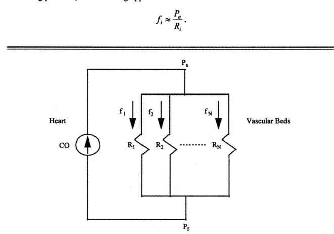
The flow of blood from the heart to the vascular beds of the many tissues can be conceptualized with the electrical circuit in Figure 2-3. This circuit illustrates that the heart and the vascular beds can be respectively thought of as a current source and resistances connected in parallel. Note that the electrical variables of the circuit are represented with their analogous cardiovascular variables. The rate of blood flow fi through the ith vascular bed is as follows:

=

P - P

Ri

where Pa is arterial pressure, Pf is the filling pressure, and Ri represents the vascular resistance of the ith _{vascular bed. Since arterial pressure is generally much greater than} the filling pressure, the following approximation can be made:

fRPa

Ri Pa Heart CO Vascular Beds

Figure 2-3: Electrical circuit model relating cardiac output (CO), arterial pressure (Pa),

filling pressure (Pf), local vascular resistance (Ri), and local blood flow (fi). Modified from [14].

(19)

Since adjustments in arterial pressure will influence blood flow to all vascular beds, the local control of blood flow must be achieved by adjusting local vascular resistance. Consequently, it is of paramount importance that arterial blood pressure remain constant or nearly constant. Otherwise, with varying arterial blood pressure, it would never be known whether adjustments in resistance would result in the appropriate changes in local blood flow. Therefore, the cardiovascular system includes a complex regulatory system that maintains arterial blood pressure within narrow limits. This is referred to as the extrinsic control of the cardiovascular system and is the focus of this thesis. It should be noted that the term cardiovascular control will henceforth refer specifically to extrinsic cardiovascular control.

The extrinsic control system consists of many control and feedback loops. The control loops are specifically responsible for adjusting arterial blood pressure via some of the cardiovascular variables that influence it. Figure 2-3 illustrates that arterial blood pressure is related to the overall blood flow from the heart or cardiac output CO and total peripheral vascular resistance R as follows:

P, =COx R

where

1 1 1 1

- = -- +-+---+ .

R R, R2 RN

Peripheral vascular resistance is adjusted by constriction or dilation of the resistance vessels respectively termed vasoconstriction (TR) or vasodilation (,R). The resistance vessels are primarily the arterioles whose thick, muscular walls allow for significant changes in caliber and thus resistance. Control of cardiac output is very complex and is dependent on many cardiovascular variables. However, it is normally adjusted by either modulation of heart rate or effective blood volume. In particular, cardiac output is a monotonically increasing function of heart rate and effective blood volume. Effective blood volume is defined to be the difference in total blood volume and the filling volume of the peripheral vasculature. Specifically, effective blood volume is adjusted by the constriction or dilation of the capacitance vessels respectively referred to as

(20)

-venoconstriction (teffective blood volume -*- CO) or venodilation (,leffective blood volume -+, CO). The capacitance vessels are the veins whose thin, muscular walls do

not provide much resistance to flow but do allow for a greater capacity for changes in filling volume. The control mechanisms for adjusting peripheral vascular resistance, heart rate, and effective blood volume are of the following three types: local control, humoral control, and neural control. This thesis specifically focuses on the neural control which is on the time scale of seconds to minutes (short-term).

The autonomic nervous system is the portion of the nervous system that controls the involuntary functions of the body and consequently, plays a major role in the neural control of the cardiovascular variables that influence arterial blood pressure. The autonomic nervous system is divided into two subsystems, the sympathetic nervous system and the parasympathetic nervous system. The sympathetic nervous system innervates the arterioles and veins of the body along with the sinoatrial node (the heart's pacemaker), atria, and ventricles of the heart. The sympathetic nervous system can be further divided based on the particular chemical receptor in the tissue receiving the neural message. The chemical receptors are of three types, namely a, 13I, and 2*. The a

receptors are present in the arterioles and veins and when stimulated, they cause vasoconstriction and venoconstriction. However, the P2 receptors are also found in the arterioles and veins and when they are stimulated, they result in the opposing effect of vasodilation and venodilation. The

P1

receptors are present in the heart and when stimulated, they increase heart rate and enhance the contractility of the heart. The parasympathetic nervous system innervates the atria and ventricles of the heart to some extent but primarily innervates the sinoatrial and atrioventricular nodes via the vagus nerve. Parasympathetic stimulation decreases heart rate and slightly decreases the contractility of the heart.

There are a couple of points to note about these two subsystems. The first point to note is that the efferent branches of the sympathetic and parasympathetic nervous systems are tonically active. For example, modulation of sympathetic activity either increases or decreases vasoconstriction and venoconstriction with respect to a certain baseline tone.

(21)

Likewise, an increase or decrease in parasympathetic activity respectively decreases or increases heart rate. The second point to note is that the sympathetic nervous system increases its activity in the upright or tilted posture, while the parasympathetic nervous system increases its activity in the supine posture.

The feedback loops of the extrinsic control system work in conjunction with the control loops to maintain arterial blood pressure under various perturbations. The baroreceptor reflex is one of the most important feedback loops that act on the time scale of seconds to minutes (short-term). Baroreceptors are stretch receptors located in the carotid sinus and the aortic arch that sense changes in mean arterial blood pressure. An increase in pressure stretches the baroreceptors and causes them to transmit signals that eventually reach the autonomic nervous system. The autonomic nervous system responds by reducing peripheral vascular resistance via vasodilatory effects and decreasing cardiac output via venodilation and a reduction in heart rate and contractility of the heart. Of course, a decrease in arterial blood pressure sensed by the baroreceptors would result in the opposite effect. It should be noted that there are other inputs to the autonomic nervous system besides arterial blood pressure such as oxygen and carbon dioxide pressures and signals from higher brain centers.

2.3 Diabetic Autonomic Neuropathy

This section provides a brief treatment of the autonomic neuropathy associated with diabetes mellitus by summarizing material in [13,15,16,17]. Diabetes mellitus is a disease marked by excessive blood sugars due to insulin deficiency. Autonomic neuropathy, a frequent complication of diabetes mellitus, is a disorder that has damaging effects on sympathetic and parasympathetic nerves. Since this thesis deals with cardiovascular control mechanisms, this section specifically emphasizes the damage of the nerves that innervate the cardiovascular system referred to as cardiovascular neuropathy. Of course, cardiovascular neuropathy can have deleterious effects on the autonomic control mechanisms of the cardiovascular system.

(22)

The morphological changes associated with diabetic autonomic neuropathy and their pathogenesis are not well understood. Few studies of changes in morphology of the autonomic nerves have been completed because of the inaccessibility of these nerves. The issue of pathogenesis is controversial as both metabolic and vascular causations have been hypothesized. However, the clinical features of diabetic autonomic neuropathy are well recognized. These clinical features are often non-specific and range from mild disturbances to severe disabilities. They include symptoms involving the cardiovascular, gastrointestinal, and urogenital systems and disturbances to thermoregulatory function and pupillary reflexes.

In particular, the clinical features of cardiovascular neuropathy include postural hypotension and resting tachycardia. Postural hypotension is defined to be a fall in systolic blood pressure of greater than 30 mmHg when moving from the supine to standing posture. When the cardiovascular control system is operating normally, the decrease in arterial blood pressure that occurs on the move from supine to standing is sensed by the baroreceptors and ultimately peripheral resistance and cardiac output is increased mainly by the sympathetic nervous system. Therefore, postural hypotension reflects damage to predominantly sympathetic nerves. Resting tachycardia is a fast heart rate at rest and probably indicates the inability to reflexively modulate heart rate as a result of autonomic nerve damage.

Standard autonomic tests based on cardiovascular reflexes to various physiological perturbations are commonly employed to assess autonomic nerve damage. These tests assume that abnormal cardiovascular reflexes not only indicate cardiovascular neuropathy but damage throughout the entire autonomic nervous system. The goal of these tests are to confirm the presence and quantitatively assess the severity of autonomic neuropathy. These tests non-invasively assess the heart rate response to such perturbations as the Valsalva maneuver (subject blows into a mouthpiece at a pressure of 40 mm Hg for 15 seconds), standing up, and deep breathing and the blood pressure response to such perturbations as standing up and sustained handgrip. Although both branches of the autonomic nervous system are involved in these tests to some extent, the sympathetic nervous system is believed to play the major role in the blood pressure tests.

(23)

However, the blood pressure tests are relatively insensitive, particularly to early sympathetic nerve damage. Furthermore, both heart rate and blood pressure tests require the active cooperation of the subject and so, the test results may be difficult to reproduce.

The prevalence and natural history of diabetic autonomic neuropathy is not fully understood. Between 17 and 40% of randomly selected diabetic subjects have abnormal standard autonomic test results according to large studies. The development of clinical features is variable and appears to be relatively late. They are slowly progressive and usually irreversible and their onset often results in severe disabilities. Studies show that diabetic subjects with clinical symptoms of autonomic neuropathy are associated with considerable mortality. The potential consequences associated with diabetic autonomic neuropathy emphasize the need for its quantification. This quantification would provide a physiological measure of the progression of autonomic nerve damage and consequently, guidance for treatment. For example, an increase in the autonomic nerve damage would indicate the need for tighter glucose control. Therefore, the standard autonomic tests are often employed clinically despite their severe drawbacks. Clearly, a more sensitive test that requires minimal subject participation is needed to quantitatively assess diabetic autonomic neuropathy.

2.4 System Identification of Cardiovascular Control Mechanisms

This section discusses some aspects involved in the application of system identification to the study of short-term cardiovascular control mechanisms and presents some highlights of previous studies. Since a major component of this thesis is diabetic autonomic neuropathy, an emphasis is placed on the study of cardiovascular control mechanisms of subjects with diabetes mellitus.

2.4.1 Simple Models of Short-Term Cardiovascular Control Mechanisms

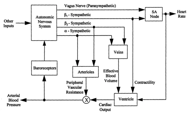
Figure 2-4 summarizes the autonomic control mechanisms of the cardiovascular system discussed in Section 2.2 in a block model The blocks of the model represent functional subsystems of the entire control system. The autonomic control mechanisms

(24)

are much too complicated for each block to be described with physical insight. However, if the input-output data to each subsystem could be measured, then system identification could be employed to estimate the dynamics of each block. Therefore, a fairly complete assessment of autonomic control would be obtained. Unfortunately, much of the input-output data in this model is not available for measurement and hence, this model is not particularly useful in the system identification context. However, some of the input-output data in this model, such as heart rate and arterial blood pressure, are easily accessible for measurement and can be used to estimate simpler models. Although, these models are not as detailed, they still provide useful insight about some aspects of

autonomic control mechanisms.

Other Inputs Arter Bloc Press Heart Rate Output

Figure 2-4: Block model of the autonomic control mechanisms of the cardiovascular system. Modified from [8].

Respiratory activity is also readily available for measurement via instantaneous lung volume. Although it is not included in the model in Figure 2-4, respiratory activity is an important factor in the study of cardiovascular control because it is a perturbation to

(25)

the cardiovascular system that causes a dynamic and compensatory response by the cardiovascular control mechanisms. Therefore, respiration can also be included in simple models of cardiovascular control. Specifically, respiration influences the cardiovascular system by perturbing both arterial blood pressure by mechanical mechanisms [8] and heart rate by autonomic mechanisms [37].

The intrathoracic pressure changes that result from respiration produce an additive effect on arterial blood pressure and modulate venous return and ventricular filling which eventually affect arterial blood pressure through their effects on cardiac output. Specifically, during inspiration, the intrathoracic pressure is more negative than usual. This causes an immediate decrease in arterial blood pressure due to capacitive effects and increases venous return to the right side of the heart which increases ventricular filling and eventually cardiac output from the left side of the heart. During expiration, the opposite effects occur.

Heart rate is also modulated by respiration. Specifically, phasic changes in heart rate follow the inspiratory and expiratory cycle of respiration. This is commonly referred to as respiratory sinus arrhythmia (RSA). The mechanisms that generate RSA are not completely understood; however, several potential mechanisms for RSA have been suggested. One possible mechanism is the direct neural coupling of the respiratory drive and heart rate control centers within the central nervous system. Another possible mechanism is the mechanical modulation of arterial blood pressure influencing heart rate via the baroreceptor reflex. Although the mechanisms for RSA are not completely understood, it is known that the modulation of heart rate in response to respiration is mediated by the autonomic nervous system almost exclusively.

2.4.2 Fluctuations in Cardiovascular Variables

It should be emphasized that when employing system identification to model the autonomic control mechanisms of the cardiovascular system, it is essential to deal with the fluctuations in cardiovascular variables such as heart rate, arterial blood pressure, and respiration about their mean values [3]. The mean values of cardiovascular variables are simple to examine and are thus used clinically, but they imply only the static state of

(26)

cardiovascular control. However, the fluctuations in cardiovascular variables about their mean values imply the dynamic nature of cardiovascular control as they represent the interplay between perturbations to the cardiovascular system and the response of cardiovascular control mechanisms. Of course, these perturbations can either be

exogenous such as respiratory activity or endogenous such as local vascular resistance adjustments which affect total peripheral resistance.

The information concerning cardiovascular control inherent in the fluctuations in cardiovascular variables is illustrated by examining the power spectrum of heart rate. Power spectral estimation decomposes a signal into a sum of sine waves of different frequencies. The power spectrum is presented as the squared amplitude of these sine waves as a function of frequency. Figure 2-5 shows that a typical heart rate power spectrum contains three peaks that are centered at approximately 0.04 , 0.1, and 0.2 Hz. The 0.2 Hz peak is associated with fluctuations in respiration and the 0.1 and 0.04 Hz peaks are probably related to fluctuations resulting from arterial blood pressure regulation. The frequency band above 0.15 Hz is modulated by the parasympathetic nervous system as power in this band disappears during parasympathetic blockade. On the other hand, the frequency band below 0.15 Hz is modulated by both sympathetic and parasympathetic nervous systems as power in this band is diminished during either blockade and completely disappears during double blockade.

(27)

1504 0 1 02 0.3 0.4 0.5 0 1 2 3 4 0.1 0.2 3 0.4 0.6 Time,hm Frm y, Hi 120 0 1 2 3 .so. 10 40' 0 1 2 3 Tim, mi 120 160 sss 0 50 S 2 0.1 02 02 OA 0. E1 Tim, *i 400 0.1 0.0. 02 0.4 0.5

Figure 2-6: The power spectrum of heart rate for a) a control, b) a diabetic subject with

moderate autonomic neuropathy, and c) a diabetic subject with severe autonomic neuropathy. Reproduced from [20].

Since the power spectrum reveals so much about autonomic control, it is natural to wonder whether it can be used as an assessment tool for autonomic neuropathy. In fact, there has been extensive work on the application of heart rate power spectral estimation to assess the autonomic neuropathy associated with diabetes mellitus

[7,20,27,33]. The total power of the heart rate spectrum decreases with increasing

autonomic neuropathy. This is consistent with the hypothesis that autonomic modulation of heart rate reduces as nerve damage progresses. Figures 2-6a, b, and c illustrate this

Nrml lH rl dao 50 0.1 0.2 0.3 0.4 0.5 25Up~t 0.1 02 0. 0.4 0. Fiquccy. Hz IF

(28)

trend by respectively showing the power spectrum of a control subject, a subject with moderate autonomic neuropathy, and a subject with severe autonomic neuropathy in both supine and upright postures. Additionally, the parameters of the heart rate power spectrum such as low frequency power, high frequency power, and total power compare well with the standard autonomic tests. Although heart rate power spectral analysis is a quantitative, non-invasive, and sensitive method that requires minimal subject participation, it only provides information about an output of a control loop of the cardiovascular control system. It does not provide any information about how the output would change to varying inputs to the control loop. Clearly, it would be more informative to estimate the dynamics of the couplings of the control and feedback loops of the cardiovascular control system from experimental data.

2.4.3 Previous Studies

Many previous studies have applied system identification to quantitatively and non-invasively assess cardiovascular control mechanisms with minimal subject participation. A few of these studies have specifically assessed the cardiovascular control mechanisms of diabetic autonomic neuropathy. Of course, none of these studies provide a complete description of cardiovascular control; however, they do provide insight about some aspects of the cardiovascular control system. It should be noted that all of these studies assumed that the cardiovascular control mechanisms behaved as LTI systems. The system identification techniques that have been employed can be divided essentially into two categories namely, nonparametric transfer function analysis and parametric system identification.

Nonparametric transfer function analysis provides an estimation of the gain and phase delay as a function of frequency between a single input and output of an LTI system. Because this type of analysis applies to LTI systems, a requirement is that the input data contains all relevant frequencies of interest so that the system can be identified at all these frequencies. The estimation procedure involves the determination of the optimal estimate of the transfer function in the least squares sense computed via

(29)

FFT-based spectral analysis. The interested reader can find a detailed treatment of this topic in [38].

Nonparametric transfer function analysis has been applied to analyze several aspects of cardiovascular control. Berger et al. stimulated the vagus and cardiac sympathetic nerves of dogs in a broadband manner to study the coupling of this stimulation and the resulting atrial rate in order to gain insight about the dynamics of the sinoatrial node [10]. They found that the sinoatrial node behaves as a lowpass filter whose cutoff frequency depends on both the mean level of stimulation and the particular nerve that was stimulated. Saul et al. examined the coupling of respiration and heart rate using techniques to broaden the frequency content of respiration in order to study RSA [35]. They determined that RSA was frequency dependent with parasympathetic nervous control providing a faster and larger heart rate response to respiration than sympathetic nervous control. The objective of study in [36] included the analysis of RSA and the coupling between respiration and blood pressure by blocking branches of the autonomic nervous system pharmacologically. One of the discoveries of this study was that the respiratory effects on arterial blood pressure are mediated by both RSA and the mechanical affects of respiration on arterial blood pressure. Freeman et al. assessed RSA in diabetic autonomic neuropathy [21]. The main results of this study are shown in Figure 2-7. Figure 2-7a shows the mean gain between respiration and heart rate as a function of frequency for groups with varying degrees of autonomic neuropathy. Specifically, the mean gain decreases as autonomic neuropathy increases across these groups for both the supine and tilted postures. Figure 2-7b illustrates the mean phase delay between respiration and heart rate as a function of frequency for these groups. The phase delay at low frequencies is particularly of interest and implies that sympathetic modulation increases (but to no avail as is evident in Figure 2-7a) with increasing autonomic neuropathy in the supine posture and plays a major role regardless of the degree of autonomic neuropathy in the tilted posture.

Clearly, nonparametric transfer function analysis provides useful insight about cardiovascular control mechanisms. However, its utility is limited. Consider the important coupling between heart rate and arterial blood pressure. This coupling is a

(30)

IRUCaRC-·li~-·i~Bau~-·~--·-··II·----closed-loop relationship in that arterial blood pressure influences heart rate by way of the autonomically mediated baroreceptor reflex, and heart rate affects arterial blood pressure via the mechanical effects of ventricular contraction. As will be shown in Section 3.4.2, causality conditions must be imposed in order to identify the open-loop couplings in a closed-loop system. Since nonparametric transfer function analysis cannot impose causality conditions, this technique cannot distinguish between the open-loop couplings in a closed-loop system. However, as will be shown in Section 3.2.1, parametric system identification can impose causality conditions. The power of parametric system identification over nonparametric transfer function analysis rests with this fact.

a) Supine Tilt b) supine

I @ 'Or 1I01 20 10 a. 0. a 21. .ii U 0.5 GA 0.1 i . 4 U~3 ~ 41rp "' "O·41J lip0 j * l U ~o 0.1 0.2 0. 0.4 0.5 0.1 0.2 0.4 0.5 12 0M

Fruepny (Mher) FRequency (herz)41

SNormalDiabe•ics oNUAS

- M uropathy

-

.,,o•

c Severe Neuropathy l * y jiwu,

Figure 2-7: a) The mean transfer function gain between respiration and heart rate for

groups with varying degrees of neuropathy in the supine and tilted postures. b) The mean transfer function phase delay between respiration and heart rate for these groups also in the supine and tilted postures with the control, normal diabetic, mild neuropathy, and severe neuropathy groups respectively arranged from top to bottom. Reproduced from [21].

Parametric system identification provides an estimation of couplings typically in the form of a parameterized impulse responses. The general estimation procedure is reviewed in Section 2.1.3. Of course, parametric system identification can also be applied to open-loop couplings. Yana et al. examined RSA by blocking branches of the autonomic nervous system pharmacologically [45]. Their technique included a method to

(31)

broaden the frequency content of respiration so as to provide informative data, pre- and post-processing procedures, a time domain, moving average (MA) difference equation, and least squares estimation. Their model estimates in the form of impulse responses implied that changes in heart rate anticipated changes in respiration. This suggests the neural coupling of respiratory drive and heart rate control centers and thus supports the role of the central nervous system in the generation of RSA. They also found that parasympathetic block almost completely diminished the impulse response while sympathetic block had little effect, perhaps indicating greater parasympathetic modulation.

As mentioned previously, the real utility of parametric system identification in the cardiovascular control context is that it can be applied to closed-loop systems. Kenet examined the closed-loop coupling of heart rate and arterial blood pressure in dogs under normal sinus rhythm and during atrial fibrillation [26]. This technique involved using a symmetric closed-loop model, autoregressive, moving average (ARMA) difference equations, and generalized least squares estimation. He found that the data was not informative enough during normal sinus rhythm; however, during atrial fibrillation this problem was resolved at the expense of normal operating conditions. Baselli et al. studied the couplings between heart rate, arterial blood pressure, and respiration [6]. Their method involved using a closed-loop model consisting of seven transfer relations and two unmeasured noise perturbations, dividing the system into two models, and generalized least-squares estimation. However, the data was not informative enough as the respiration data was not persistently exciting. Appel et al. also examined the couplings between heart rate, arterial blood pressure, and respiration under selective pharmacological blockade of autonomic pathways [4]. This method involved a random-interval breathing technique to provide informative data, a closed-loop model consisting of four transfer relations and two unmeasured noise perturbations, ARMA difference equations, and least squares estimation. Their method was able to distinguish between altered autonomic states produced by both postural changes and the pharmacological blockade. Additionally, their results were consistent with established physiological

(32)

---~---experimental results. This thesis, in fact, implements this same method to study aspects of the cardiovascular control mechanisms of patients with diabetic autonomic neuropathy.

(33)

Chapter 3 Closed-Loop System Identification

Procedure

This chapter describes the closed-loop system identification procedure that is implemented to assess diabetic autonomic neuropathy. The chapter presents this procedure in the context of the general system identification procedure in Section 2.1.3. Specifically, input-output data generation, candidate model selection, "best" model determination, and model validation are all discussed in some detail.

3.1 Generation of Input-Output Data

The first step in any system identification procedure is to create the input-output data. This step includes experiment design and data collection and processing. The objective is to generate the most informative, cleanest data possible so that good models can be constructed.

3.1.1 Experiment Design

Experiment design deals with such issues as what signals to measure, under what conditions are these signals to be measured, and whether these signals are related in

(34)

open-or closed-loop. Since heart rate, arterial blood pressure (ABP), and instantaneous lung volume (ILV) signals are all easily accessible and identification of their couplings can provide useful insight about cardiovascular control mechanisms, these signals are chosen for measurement. Strictly speaking, heart rate is not readily available, but it can be derived from the surface electrocardiogram (ECG) which is perhaps the easiest cardiovascular signal to measure. Therefore, the ECG, ABP, and ILV signals are actually chosen for measurement. These signals are measured during two sessions, first while the subject is supine and then following passive tilting to 600 (relative to the supine posture) by an electrically driven tilt table. Each posture provides a different balance between sympathetic and parasympathetic control of the cardiovascular system. Consequently, the measurements from each session may be very insightful about the roles of the sympathetic and parasympathetic nervous systems in cardiovascular control. Before each of these sessions, the subject is provided with a period of hemodynamic equilibration. Approximately eight minutes of data are measured for each session as it is short-term cardiovascular control mechanisms that will be assessed. It should be emphasized that this is a closed-loop experiment because of the relationship between heart rate and ABP.

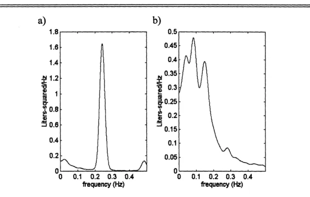
The goal of experiment design is to obtain maximally informative data. Informative data results from persistently exciting inputs, and in practice, persistently exciting inputs correspond to broadband inputs. (This issue will be discussed further in Section 3.4.2.) Heart rate and ABP can be thought of as outputs of the cardiovascular control system; however, ILV is an exogenous input to this system. Therefore, it is essential for ILV to be broadband. Unfortunately, normal breathing patterns typically result in narrowband ILV data. As a result, during both sessions, subjects are instructed to breathe on cue according to a sequence of auditory tones spaced by independent and identically distributed, modified exponential inter-breath times. The inter-breath times range from one to 15 seconds with a mean of five seconds to avoid subject discomfort. This "random-interval breathing technique" provides broadband ILV data within 0.5 Hz while preserving normal ventilation [9]. Figure 3-1 illustrates the effectiveness of the

(35)

random-interval breathing technique by showing the power spectra of ILV generated by normal breathing and random-interval breathing.

1 .0 0.2 0.3 0.4

1 .0 0.2 0.3 0.4 frequency (Hz) frequency (Hz)

Figure 3-1: ILV breathing.

power spectra from a) normal breathing and b) random-interval

3.1.2 Data Collection and Processing

The collection and processing of data involves the measurements and signal processing techniques included in the generation of the input-output data. The ECG, ABP, and ILV signals are measured non-invasively and recorded continuously on a Teac

C-71, eight-channel FM tape recorder (Teac America, Montebello, CA). The ECG signal

is measured with a Hewlett-Packard EKG Monitor 78203A (Andover, MA); the ABP signal is measured with a 2300 Finapress Continuous Blood Pressure Monitor (Ohmeda, Fort Lee, NJ); and the ILV signal is measured with a two-belt chest-abdomen inductance pelthysmograph (Respitrace System, Ambulatory Monitoring, Inc., Ardsley, NY). The ILV signal is calibrated by having the subject alternately empty and fill an 800 ml bag after each period of hemodynamic equilibration. These three signals are then lowpass

cr 4, I-U) -J 0 0.1 0.2 0.3 0.4

(36)

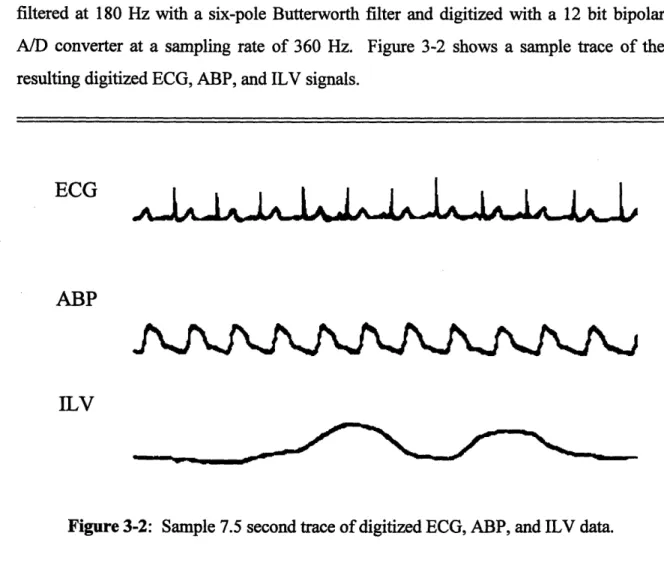
filtered at 180 Hz with a six-pole Butterworth filter and digitized with a 12 bit bipolar A/D converter at a sampling rate of 360 Hz. Figure 3-2 shows a sample trace of the resulting digitized ECG, ABP, and ILV signals.

ECG

ABP

ILV

Figure 3-2: Sample 7.5 second trace of digitized ECG, ABP, and ILV data.

The couplings of the three digitized signals can be described with the closed-loop model of short-term cardiovascular control illustrated in Figure 3-3. The model represents the closed-loop coupling of heart rate and ABP with ILV as an exogenous perturbation that directly influences both heart rate and ABP. Since, it is assumed that heart rate and ABP do not affect ILV, these couplings are not included in the model. Therefore, the model contains four unknown open-loop couplings or transfer relations (ILV-+HR, BAROREFLEX, ILV--ABP, and CIRCULATORY MECHANICS) and two unmeasured noise perturbations (NHR and NABp). ILV--HR represents the autonomic coupling between ILV and heart rate or equivalently, RSA. BAROREFLEX represents the effects of ABP on heart rate due to the autonomically mediated baroreceptor reflex. ILV-+ABP represents the mechanical coupling between ILV and ABP resulting from variations in intrathoracic pressure induced by respiration producing an additive effect on

(37)

ABP and modulating venous return and ventricular filling which indirectly affect ABP. CIRCULATORY MECHANICS primarily represents the mechanical effects of a single ventricular contraction on the ABP waveform. However, the autonomic nervous system also has some influence on CIRCULATORY MECHANICS since the ABP waveform is dependent on peripheral vascular resistance which is sympathetically mediated. NHR and NABP respectively represent the residual variation in HR and ABP not accounted for by the couplings.

NHR

I

(ILV) Arterial Blood

sure IP)

NAs,

Figure 3-3: Closed-loop model of short-term cardiovascular control mechanisms relating

heart rate, ABP, and ILV.

(38)

~-C-·PIIII~-~·-L111~··-·111-An additional transfer relation (SA NODE) is also included in the model. SA NODE reflects the effects of autonomic tone (represented by a heart rate tachogram (HR)) on the modulation of the timing of ventricular contractions (represented by an impulse heart rate (IHR) signal) by the sinoatrial node. Since the dynamics of the sinoatrial node are well described via the integral pulse frequency modulation (IPFM) model [25] and HR and IHR can be derived from the ECG as described in [11] and illustrated in Figure 3-4, SA NODE is not estimated. The SA NODE is essential to the model, though. The autonomic modulation of HR is over the spectral band between dc and roughly 0.35 Hz [31 ], while the spectral content of the ABP waveform includes up to the tenth harmonic of the mean heart rate which is usually about 10 Hz [12]. However, it will be assumed that the couplings are LTI and so, the output can only contain power at frequencies that are excited by the input. Because the spectral content of IHR also includes at least up to the tenth harmonic of the mean heart rate, the function of SA NODE is to close the loop by converting HR to IHR which is in turn linearly coupled to the ABP waveform. Thus, SA NODE is a fully defined nonlinear element which is crucial to the closed-loop model but does not require estimation.

It will be discussed in Section 3.3.1 that the couplings and noise perturbation involved in the generation of HR will be estimated separately from the couplings and noise perturbation involved in the creation of ABP. The signals used for the estimation of the former couplings and noise perturbation are HR, ABP, and ILV. This data is zero-meaned and decimated to 1.5 Hz which is more than sufficient to accommodate the spectral content of the autonomic modulation of HR. The longest portion of the eight minute data segment that is clean is used for this estimation. The signals used for the estimation of the latter couplings and noise perturbation are ABP, IHR, and ILV. This data is zero-meaned and decimated to 90 Hz which provides more than enough bandwidth for the ABP waveform. Ninety seconds of the cleanest portion of the eight minute data segment is used for this estimation. Additional processing techniques will be necessary in the closed-loop system identification procedure; however, these techniques will be discussed in Section 3.4.3.

(39)

HR Tachogram

ECG

IHR Signal

-I

--Figure 3-4: Derivation of the heart rate tachogram (HR) and the impulse heart rate signal (IHR) from the ECG. The units of ECG are in millivolts (mV), while IHR has arbitrary units.

3.2 Least Squares Estimation

The next step of the general system identification procedure deals with the selection of a candidate set of models. However, the fundamental concepts of least squares estimation are presented here, because they are essential to understanding this step and the remaining steps of the closed-loop system identification procedure. Least squares estimation is an identification method that is used in this thesis as a tool for the determination of the "best" model. Since the closed-loop system identification procedure employs LTI systems in the form of difference equations, this section specifically focuses on least squares estimation in this context.

Time

I I I

JeNý

_{-- 411w}

~---"~""""""I"~~""11~""~"11--~ T,

I

T2

(40)

3.2.1 LTI Systems

Disregarding any disturbances, a system is a transformation T{.} that maps an input u(t) to an output y(t) i.e.,

y(t) = T{u(t)}.

A linear system follows the principle of superposition which states that

T{au,(t)+ bu2(t)} = aT{u,(t)} + bT{u2(t)}

where ul(t) and u2(t) are inputs to the linear system and a and b are arbitrary constants. A time-invariant system is one in which a time shift of the input produces the identical time shift of the output. Equivalently, provided that the output y(t) of a system results from the input u(t), a system is time-invariant if the input u(t-to) produces the output y(t-to). The input-output relationship of an LTI system is described by the convolution operation

as follows:

y(t) = h(k)u(t - k) = h(t)* u(t)

k

where * denotes the convolution operator and h(t) is referred to as the impulse response of the LTI system. Note that if the impulse response of an LTI system is known, then for any input to that system, the output can be determined. In other words, the impulse response completely characterizes an LTI system. This is a powerful feature of LTI analysis.

An important subclass of LTI systems are linear constant coefficient difference equations (LCCDE's). The general form of such a difference equation with input u(t) and

output y(t) is

R S

Z

,aky(t- k)=

bku(t-

k).

k=R' k=S'

where R' < 0. Note that if R' = 0 and S" > 0, the system is causal. This general form is often referred to as an autoregressive, moving average (ARMA) equation. Assuming

R' = 0, the autoregressive (AR) portion of this equation deals with past values of the output influencing the present value of the output. The moving average (MA) portion of