HAL Id: hal-00317781
https://hal.archives-ouvertes.fr/hal-00317781
Submitted on 22 Dec 2004
HAL is a multi-disciplinary open access
archive for the deposit and dissemination of
sci-entific research documents, whether they are
pub-lished or not. The documents may come from
teaching and research institutions in France or
abroad, or from public or private research centers.
L’archive ouverte pluridisciplinaire HAL, est
destinée au dépôt et à la diffusion de documents
scientifiques de niveau recherche, publiés ou non,
émanant des établissements d’enseignement et de
recherche français ou étrangers, des laboratoires
publics ou privés.
precipitation-related variations in the behaviour of
SuperDARN Doppler spectral widths
M. L. Parkinson, G. Chisham, M. Pinnock, P. L. Dyson, J. C. Devlin
To cite this version:
M. L. Parkinson, G. Chisham, M. Pinnock, P. L. Dyson, J. C. Devlin. Magnetic local time, substorm,
and particle precipitation-related variations in the behaviour of SuperDARN Doppler spectral widths.
Annales Geophysicae, European Geosciences Union, 2004, 22 (12), pp.4103-4122. �hal-00317781�
SRef-ID: 1432-0576/ag/2004-22-4103 © European Geosciences Union 2004
Annales
Geophysicae
Magnetic local time, substorm, and particle precipitation-related
variations in the behaviour of SuperDARN Doppler spectral widths
M. L. Parkinson1, G. Chisham2, M. Pinnock2, P. L. Dyson1, and J. C. Devlin3 1Department of Physics, La Trobe University, Victoria 3086, Australia
2British Antarctic Survey, Natural Environment Research Council, Cambridge CB3 0ET, UK 3Department of Electronic Engineering, La Trobe University, Victoria 3086, Australia
Received: 20 August 2003 – Revised: 23 June 2004 – Accepted: 5 October 2004 – Published: 22 December 2004
Abstract. Super Dual Auroral Radar Network (DARN) radars often detect a distinct transition in line-of-sight Doppler velocity spread, or spectral width, from <50 m s−1 at lower latitude to >200 m s−1 at higher latitude. They also detect a similar boundary, namely the range at which ionospheric scatter with large spectral width suddenly com-mences (i.e. without preceding scatter with low spectral width). The location and behaviour of the spectral width boundary (SWB) (and scatter boundary) and the open-closed magnetic field line boundary (OCB) are thought to be closely related. The location of the nightside OCB can be in-ferred from the poleward edge of the auroral oval determined using energy spectra of precipitating particles measured on board Defence Meteorology Satellite Program (DMSP) satellites. Observations made with the Halley SuperDARN radar (75.5◦S, 26.6◦W, geographic; −62.0◦3)and the Tas-man International Geospace Environment Radar (TIGER) (43.4◦S, 147.2◦E; −54.5◦3)are used to compare the loca-tion of the SWB with the DMSP-inferred OCB during 08:00 to 22:00 UT on 1 April 2000. This study interval was chosen because it includes several moderate substorms, whilst the Halley radar provided almost continuous high-time resolu-tion measurements of the dayside SWB locaresolu-tion and shape, and TIGER provided the same in the nightside ionosphere. The behaviour of the day- and nightside SWB can be under-stood in terms of the expanding/contracting polar cap model of high-latitude convection change, and the behaviour of the nightside SWB can also be organised according to substorm phase. Previous comparisons with DMSP OCBs have proven that the radar SWB is often a reasonable proxy for the OCB from dusk to just past midnight (Chisham et al., 2004). How-ever, the present case study actually suggests that the night-side SWB is often a better proxy for the poleward edge of Pedersen conductance enhanced by hot particle precipitation in the auroral zone. Simple modeling implies that the large spectral widths must be caused by ∼10-km scale velocity fluctuations.
Correspondence to: M. L. Parkinson
Key words. Ionosphere (auroral ionosphere;
ionosphere-magnetosphere interactions) – Magnetospheric physics (storms and substorms)
1 Introduction
Changes in the latitude and shape of the open-closed mag-netic field line boundary (OCB) are a direct indication of en-ergy coupling in the solar wind-magnetosphere-ionosphere system. The dynamics of the OCB can be understood in the context of the expanding/contracting polar cap model of high-latitude convection change (Siscoe and Huang, 1985; Cowley and Lockwood, 1992). This mechanistic model ex-plains how the area of the polar cap ionosphere, or the geo-magnetic region open to the IMF, inflates when dayside re-connection proceeds at a faster rate than nightside reconnec-tion, and conversely, deflates when reconnection in the tail dominates. The behaviour of the OCB can also be under-stood in the context of the global substorm instability, namely the cyclic but poorly understood loading and unloading of energy in the magnetotail (Baker et al., 1999; Lui, 2001).
Thus, it is very important to determine if, and when, vari-ous features observed by different ground-based instruments, for example, the Doppler spectral width boundary (SWB) ob-served by Super Dual Auroral Radar Network (SuperDARN) radars, correspond to the OCB under a broad range of geo-physical conditions, including ionospheric substorms. Other proxies for the OCB include the poleward edge of 630.0-nm auroral emission (Blanchard et al., 1997), and the poleward edge of the auroral oval measured in situ by spacecraft (Vam-pola, 1971; Evans and Stone, 1972). For example, the OCB can be inferred from spectrograms of precipitating particles measured on board the Defense Meteorological Satellite Pro-gram (DMSP) spacecraft.
The SuperDARN network of HF backscatter radars was established to monitor high-latitude ionospheric convection on a global scale (Greenwald et al., 1985, 1995). Super-DARN presently consists of 9 radars encircling the north-ern polar cap, and 7 radars encircling the southnorth-ern polar cap.
Each radar employs a 16-element, 240-m wide phased an-tenna array to produce an ∼4◦-wide main beam (at 12 MHz).
During routine operation, this beam is sequentially stepped through 16 directions separated in azimuth by 3.24◦, thereby forming a ∼52◦-wide field of view (FOV).
Bragg-type backscatter is obtained from ionospheric irreg-ularities with a field-perpendicular scale size equal to half the radio-wavelength, equal to 12.5 m at 12 MHz. Basic echo parameters, including the backscatter power, line-of-sight (LOS) Doppler velocity, and Doppler velocity spread (or “spectral width”), are calculated using “FITACF,” an al-gorithm which fits Gaussian and Lorentzian functions to the autocorrelation functions (Baker et al., 1995). During routine operation, FITACF parameters are usually recorded once ev-ery 1–2 min at any of 70 ranges between 180 to 3330 km in 45-km steps.
The backscatter power is a measure of the number and relative intensity of electron density irregularities within the ionospheric sampling volume (Parkinson et al., 2003a), as well as the effects of ionospheric absorption, and focusing and defocusing of the radio beams. The LOS Doppler veloc-ities are a measure of field-perpendicular electric fields when the backscatter emanates from the F-region of the ionosphere (Villain et al., 1985) and the upper E-region (Parkinson et al., 1997). Lastly, the spectral widths are a measure of the life-time of ionospheric irregularities, as well as space and life-time variations in the LOS Doppler velocity occurring within the sampling volume and integration time.
Non-uniform convection flows from small (∼1 km) to large scales (∼1000 km) (Parkinson et al., 1999), micro-scale (∼10 m) plasma turbulence, and electric field variations in the Pc 1-2 frequency range, may all play a possible role in in-creasing the radar spectral widths. However, the large spec-tral widths encountered in the auroral and cusp ionosphere cannot be explained by large-scale variations in the convec-tion pattern (Andr´e et al., 2000b). Andr´e et al. (1999, 2000a) modeled the SuperDARN measurement process and argued that the large spectral widths are caused by electric field variations in the Pc 1–2 frequency range. However, Pono-marenko and Waters (2003) found an error in the calculus of Andr´e et al. The small-scale process causing large spectral widths observed in the cusp and nightside ionosphere is still an open question.
A distinct transition in spectral width from <50 m s−1at lower latitude to >200 m s−1 at higher latitude is often ob-served in the dayside ionosphere. This spectral width bound-ary (SWB) has been interpreted as a proxy for the open-closed magnetic field line boundary (OCB) when the inter-planetary magnetic field (IMF) Bz component is southward
(Baker et al., 1995; Milan et al., 1998; Moen et al., 2001). The dayside scatter with large spectral widths expands equa-torward and contracts poleward when the IMF Bzcomponent
increases and decreases, respectively (Pinnock et al., 1993). Chisham et al. (2001) observed an equatorward expansion of a dayside bulge in the SWB, perhaps signifying the ac-cumulation of open flux during dayside reconnection when the IMF Bycomponent changed in sign. On the other hand,
the SWB sometimes exhibits a poleward directed, bay-like feature in proximity to the cusp (Pinnock and Rodger, 2001). Chisham et al. (2002) argued that these bays indicate that the SWB is sometimes displaced poleward of the true OCB because of “the poleward motion of newly-reconnected mag-netic field lines during the cusp ion travel time from the re-connection X-line to the ionosphere”. Associating the radar SWB with an ionospheric precipitation boundary implies it may not always be exactly coincident with the instantaneous location of the OCB.
SuperDARN radars often observe a similar SWB in other magnetic local time (MLT) sectors, including the midnight auroral ionosphere. Recently, the interpretation of the night-side SWB has varied. Early work suggested it corresponds to the boundary between the central plasma sheet (CPS) and the so-called boundary plasma sheet (BPS) (Lewis et al., 1997, 1998; Dudeney at al., 1998). More recent studies suggest that the nightside SWB may actually correspond to the OCB under favourable conditions (Lester et al., 2001; Parkinson et al., 2002b, 2003b1). However, after comparing EISCAT and CUTLASS radar data, Woodfield et al. (2002a, b) ques-tioned whether the SWB was a reliable proxy for the OCB in the post-midnight sector.
Thus, the purpose of this paper is threefold, namely to further investigate (i) problems associated with identifying the SWB, including the all-important effects of HF propaga-tion, (ii) whether the nightside SWB is a reliable proxy for the OCB in different MLT sectors and for various geomag-netic activity levels, including ionospheric substorms, and (iii) the behaviour of the nightside SWB with respect to the behaviour of the dayside SWB in the context of the expand-ing/contracting polar cap model of high-latitude convection change. Thereby we gain further insights into the cause and true identity of the SWB.
To these ends, we analyse dual SuperDARN radar mea-surements made on 1 April 2000 containing ∼12 h of contin-uous day- and nightside ionospheric scatter with persistent SWBs. We compare and contrast the SWBs with the pole-ward edge of the auroral oval identified from spectrograms of precipitating particles measured on board the DMSP space-craft. The dayside SWB responded rapidly to changing IMF and solar wind conditions, and in ways closely related to that expected for the dayside OCB, and the behaviour of the nightside SWB was organized according to substorm phase. However, the comparison with energetic precipitating parti-cles measured on board DMSP, combined with a synthesis of observations reported elsewhere, actually suggests that the nightside SWB is often a better proxy for the poleward edge of height-integrated Pedersen conductivity enhanced by hot particle precipitation in the auroral zone.
1Parkinson, M. L., Pinnock, M., Dyson, P. L., and Devlin, J. C.:
Signatures of the nightside open-closed magnetic field-line bound-ary during moderately disturbed conditions and ionospheric sub-storms, Adv. Space Res., submitted, 2003b.
2 Experiment
Observations reported here were made with the Halley Su-perDARN radar (75.5◦S, 26.6◦W, geographic; −62.0◦3) and the Tasman International Geospace Environment Radar (TIGER) (43.4◦S, 147.2◦E; −54.5◦3) (Dyson and De-vlin, 2000). Magnetic latitudes given here were calculated using altitude adjusted corrected geomagnetic co-ordinates (AACGM) (Baker and Wing, 1989). Because of Halley’s more poleward location, it is more favourably located for ob-servation of the dayside cusp than TIGER; conversely, the TIGER radar is more favourably located to observe the auro-ral ionosphere in the midnight sector. Note that the spectauro-ral widths located in the pre-noon cusp are typically larger than those located in the nightside ionosphere (Villain et al., 2002; Parkinson et al., 2003a).
Figure 1 shows two scans each of the Halley (red) and TIGER (blue) radars mapped to co-ordinates consisting of MLT and AACGM latitude. The mapping to true ground range assumes a virtual reflection height of 300 km. These scans were made at different UTs, chosen to illustrate vari-ous features in the spectral widths to be discussed later. In reality, the FOVs of the two radars are located nearly diamet-rically opposite the AACGM pole.
In Fig. 1, for example, the Halley scan at 17:03:40 UT shows very large spectral widths (>300 m s−1)which must be located just poleward of the region mapping to reconnec-tion under these strong Bz southward conditions (Baker et
al., 1995; Milan et al., 1998; Moen et al., 2001). However, very low spectral widths (<100 m s−1)were present in the central polar cap ionosphere, and this provides an important clue about the mechanism regulating the spectral widths. The TIGER scan at 10:04:04 UT shows a dramatic equatorward tilt of the SWB/scatter boundary in the pre-midnight sector, and the scan at 14:09:35 UT shows extensive regions of low spectral width (<100 m s−1)equatorward of the SWB.
The chosen study interval, 08:00 to 22:00 UT on 1 April 2000 (see Fig. 3), is noteworthy because of the persistent ionospheric scatter with clear SWBs recorded concurrently by both radars. Both radars also ran high-time resolution “camping” beams. Halley beam 8 and TIGER beam 4 soundings were interleaved between routine 16-beam scans. The chosen integration time was 3 s, so the total scan time was 16×2×3 s=96 s (but slightly longer when allowing for housekeeping by the radar operating system). Halley beam 8 and TIGER beam 4 are magnetic meridian pointing beams, and are the most useful beams for accurately defining the SWB when it is magnetic L-shell aligned.
Chisham and Freeman (2003, 2004) (C-F hereafter) ex-plain an improved method of identifying the radar SWB. They emphasise the importance of applying spatial and tem-poral median filters to prevent spurious fluctuations in spec-tral width causing miss-identification of the SWB. They also emphasise the importance of choosing a spectral width threshold about half-way between the median values of the spectral width distributions occurring above and below the SWB. We used a slightly modified version of the C-F
algo-Fig. 1. Spectral widths recorded during two scans each of the Halley
and TIGER radars mapped to co-ordinates consisting of MLT and AACGM latitude. Magnetic noon (12 h) is at top, magnetic dawn (6 h) to the right, and UT at TIGER is also indicated. Halley beam 8 and TIGER beam 4 are shown in bold black. The Halley full scans commenced at 11:16:00 and 17:03:40 UT, and the TIGER full scans commenced at 10:04:04 and 14:09:35 UT. Equipotentials given by the DMSP satellite-based Ionospheric Convection Model (DICM) (Papitashvili and Rich, 2002) for (Bx, By, Bz)=(7, −4, 2) nT are
also superimposed (dotted). The minimum electric potential in the dusk cell is −27.8 kV, the maximum potential in the dawn cell is 5.5 kV, and contours are separated by 2.5 kV.
rithm 3 to analyse our measurements. It was impractical to apply an initial spatial filter across adjacent beams because of the high-time resolution camping beams. This was partly compensated for by applying a median filter to 5 consecutive beams in the time domain at every range. This reduced the time resolution to ∼30 s. The integrity of individual samples would need checking to infer behaviour of the spectral width boundary on shorter time scales.
The C-F results suggested that a spectral width thresh-old of ∼150 m s−1 or more is better suited for identifying the SWB using dayside cusp data recorded by Halley. A statistical analysis of Halley nightside data (Chisham et al., 2004) suggested that a threshold of 250 m s−1achieved
bet-ter agreement with the poleward edge of the nightside auro-ral oval, and thus the OCB. However, Fig. 9 of Parkinson et al. (2003a) suggested that a threshold as low as ∼38 m s−1 may be better suited for identifying the SWB in nightside data recorded by TIGER. The actual choice of threshold is not critical when the SWB is sharp and delineates a transition between well-separated spectral width distributions. Here we used a nominal threshold of 150 m s−1for both Halley and TIGER radar data, but the actual value chosen does not ef-fect the overall interpretation of our results.
Because of TIGER’s more equatorward location, the miss-identification of slow, subauroral ionospheric scatter as ground scatter is a significant concern. In the case of TIGER,
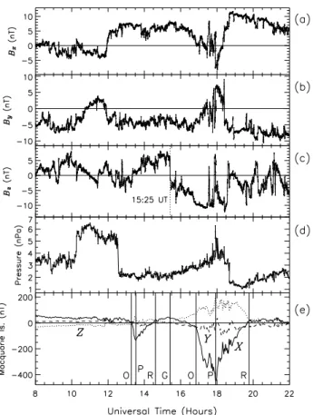
Fig. 2. ACE spacecraft measurements of the IMF (a) Bx, (b) By,
and (c) Bzcomponents, and (d) the solar wind dynamic pressure,
during 08:00 to 22:00 UT on 1 April 2000. The IMF samples are shown at 16-s resolution and the dynamic pressures at 64-s res-olution. (e) Perturbations of the geomagnetic X (solid curve), Y (dashed curve), and Z (dotted curve) components measured by the Macquarie Is. (MQI) magnetometer (provided courtesy of Geo-science Australia).
the majority of ground scatter actually emanates from the sea. Note that including sea scatter in the C-F algorithm shifts the SWB slightly equatorward. However, we could not prove when sea scatter was actually ionospheric scatter, so it was not included when estimating the SWB location. The SWB identified using the C-F algorithm has been superimposed on all full-scan data shown in Fig. 1 (black on white curves).
Changes in the energy spectra and pitch-angle distribu-tions of precipitating particles at the poleward edge of the au-roral oval indicate the location of the OCB (Vampola, 1971; Evans and Stone, 1972). Here we compare the location of radar SWBs with the results of analyzing energy spectra of precipitating particles measured on board the DMSP satel-lites, inserted in near polar orbits at an altitude of ∼830 km and a period of 101 min (e.g. Anderson et al., 1997). The nightside auroral oval boundaries shown here were those ob-tained by applying the logical criteria of Newell et al. (1996) to the energy spectra. Using the Newell et al. nomenclature, the most equatorward of the electron (b1e) or ion boundaries (b1i) was taken as the equatorward boundary of the
auro-ral oval, and the most poleward of the electron (b5e) or ion boundaries (b5i) was taken as the poleward boundary (i.e. a low-altitude proxy for the OCB).
Auroral oval boundaries were obtained using four DMSP satellites, F12, F13, F14, and F15, during our study inter-val. Because these satellites are in Sun-synchronous orbits, they favour observations made at certain local times, and rel-atively few passes were directly through the TIGER FOV. To increase the number of boundaries suitable for compari-son with the radar measurements, we considered all bound-aries identified within 2 h MLT of the beam 4 longitude (i.e. 147.2◦±30◦E). In practise, only 2 out of the 10 DMSP boundaries used here were identified outside the radar FOV, and each DMSP boundary was compared with the radar SWB identified on the nearest spatially coincident beam.
Five errors were involved in comparing the DMSP and radar boundaries: (1) the error in estimating the OCB from the DMSP energy spectra because of ambiguities in deter-mining the separation between auroral oval and polar cap precipitation, probably <1◦, (2) the small error in map-ping the DMSP measurements to magnetic latitude, proba-bly <0.5◦, (3) the error in mapping the radar scatter from group range to magnetic latitude, probably <1◦, (4) the error in defining the location of the radar SWB, probably <1◦, and (5) the error due to real fluctuations in either boundary that were too rapid in space and time to resolve, again probably <1◦. Hence adding these errors in quadrature,√4.25◦≈2◦, we obtain a plausible estimate of the maximum possible error when comparing the OCBs with the SWBs.
3 Results
3.1 Solar wind and geomagnetic conditions
Figure 2 summarises the solar wind and geomagnetic condi-tions during the chosen study interval, 08:00 to 22:00 UT, 1 April 2000. Parts (a) to (c) show the IMF Bx, By, and Bz
components in geocentric solar magnetospheric (GSM) co-ordinates, respectively, and part (d) shows the solar wind dy-namic pressure. The IMF values were measured at 16-s reso-lution on board the Advanced Composition Explorer (ACE) spacecraft, located at GSM x, y, and z co-ordinates of 227.9, −34.6, and −3.4 Re, respectively. The solar wind parameters were advected to ionospheric arrival times using GSM x dis-tances, whilst considering simultaneous IMP 8 and HF radar measurements, as explained by Parkinson et al. (2002c). The average time delay between ACE and the noon sector iono-sphere was ∼58.5 min.
The IMF By component was mostly in the range −3 to
−6 nT during the study interval, except during ∼10:45 to 11:55 UT and ∼17:15 to 18:25 UT. The variation of Bzwas
more complicated, but was mostly positive during ∼07:55 to 11:00 UT. It then underwent a succession of brief south-ward turnings to Bz∼−4 nT during ∼11:00 to 13:21 UT. It
then became strongly positive until 15:25 UT when a ma-jor, sharp, southward turning took place. The initial step-like
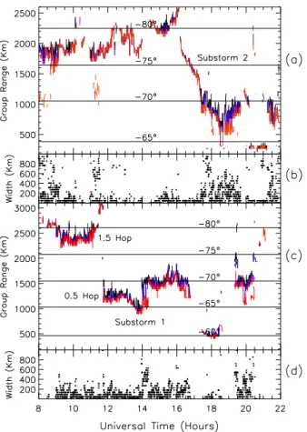
Fig. 3. Range-time plots of radar spectral widths measured on (a) Halley beam 8 and (b) TIGER beam 4 at 6-s time steps during 08:00 to
22:00 UT, 1 April 2000. Ground scatter generally has very low spectral widths and was not included in these plots. Significant changes in the operating frequency of TIGER occurred at 09:00 and 21:00 UT. Bold, fluctuating curves delineate the spectral width boundaries (SWBs) identified using the C-F algorithm with a threshold of 150 m s−1. The thin horizontal lines represent magnetic latitudes between −65◦and −85◦, and corresponding MLTs are shown at the top of each panel.
decrease was to nearly −5 nT, but was followed by a more gradual decline to −11 nT until 17:25 UT, when Bz again
began to trend back northward.
Four major features can be identified in the solar wind dynamic pressure: (1) a step-like increase from ∼3 to 6 nPa at ∼10:15 UT, (2) a step-like decrease from ∼5 to 2 nPa 12:35 UT, (3) a gradual rise to a peak of 6.3 nPa at 17:56 UT, and (4) a step-like decrease from 3.5 nPa to 1.5 nPa at 18:40 UT. Although these pressure pulses are substantial, they produced relatively short-lived transients in the radar data (Thorolfson et al., 2001). A detailed analysis of their effects is beyond the scope of this study.
Figure 1 shows the location of Macquarie Island (MQI) (54.5◦S, 158.9◦E; −65◦3) at the time of the TIGER full scan, 14:09:35 UT. MQI always maintains the same position relative to the fixed TIGER FOV. MQI fluxgate magnetome-ter measurements provide the most relevant measure of local auroral electrojet activity. Figure 2e shows MQI magnetome-ter perturbations in the geomagnetic X (north), Y (east), and Z (down) components. These were calculated by transform-ing the absolute values to AACGM co-ordinates, and then de-trended by subtracting the daily means.
Two substorms occurred during the evening of 1 April 2000. The onset (O) of a first small substorm occurred
at 13:17 UT, the peak expansion phase (P) at 13:32 UT (∼−122 nT), and the recovery phase ended (R) near ∼14:37 UT. The growth phase (G) of a second, mod-erate substorm commenced near 15:25 UT, the onset near 16:51 UT, the peak expansion phase at 17:56 UT (∼−413 nT), and the recovery phase ended near ∼19:46 UT. The ratio of Z to X perturbations indicate the westward cur-rent flow maximised almost directly above MQI for the first substorm, but just poleward of MQI for the second substorm. Whilst the accuracy of the substorm timings was not critical to the interpretation of our results, they were checked against CANOPUS magnetometer array and Los Alamos National Laboratory (LANL) satellite measurements of energetic par-ticle injections.
3.2 Dual radar measurements and spectral width bound-aries
Figure 3 shows group range versus UT plots of the radar spectral widths measured at 6-s time steps using the high-time resolution camping beam 8 for Halley (a) and beam 4 for TIGER (b). The Halley observations span the dayside in-terval, ∼6 to 18 MLT, whereas the TIGER observations span the nightside interval, ∼19 to 08 MLT. The SWBs automat-ically identified using the C-F algorithm are superimposed
Fig. 4. Range-time plots of the radar spectral width boundaries
(SWBs) identified on (a) Halley beam 8 and (c) TIGER beam 4 dur-ing 08:00 to 22:00 UT, 1 April 2000. The SWBs are shown for three different values of the spectral width threshold, namely 50 m s−1 (red), 100 m s−1(blue), and 150 m s−1(black). The thin horizontal lines represent magnetic latitudes between −60◦and −80◦. Cor-responding differences in the SWB locations using thresholds of 50 m s−1and 150 m s−1are shown in parts (b) and (d).
as bold, black curves in both parts. They fluctuate over ∼1◦ of latitude on short time scales, though still consis-tent with the separation of regions with low spectral width (<150 m s−1; black and blue) from regions of high spectral width (>150 m s−1; green and red).
It would not be possible to explain all of the short-scale fluctuations apparent in Fig. 3 in this paper. Only major vari-ations in the SWB are summarised as follows:
Halley Beam 8: During 08:00 to 15:25 UT the IMF Bz
component was mostly northward, though with brief south-ward excursions, and the SWB gradually receded polesouth-ward. During 08:00 to 13:50 UT the location of the SWB fluctu-ated rapidly with a succession of poleward contractions up to ∼2◦3, but it was mostly located between −76◦to −81◦3. During ∼13:50 to 15:25 UT the Bzcomponent was strongly
northward and during 14:20 to 15:25 UT the SWB was found further poleward at ∼−81◦3. A major Bzsouthward turning
arrived at 15:25 UT (Fig. 2c), and the SWB began to contract poleward, reaching −85◦3at 16:10 UT. However, simulta-neously, the SWB began a dramatic, 13.5◦equatorward
ex-pansion, reaching −67.5◦3at 18:35 UT. Beyond this time
Bzwas trending northward again, and the SWB began to
con-tract poleward again.
TIGER Beam 4: During 09:00 to 10:45 UT the SWB was located at approximately −78◦3. Beyond this time the SWB trended poleward, reaching −85◦3at 11:35 UT. The SWB suddenly jumped equatorward to −70◦3at 11:40 UT. The transition was unrelated to transitions in the solar wind pressure, the nearest major changes occurring at ∼10:15 and 12:35 UT. Nor was it related to changes in the transmitter fre-quency which was steady near 11.715 MHz. This transition represents a sudden change from a scatter boundary detected via 1.5-hop propagation to a true SWB detected via 0.5-hop propagation. It occurs because of a reproducible change in HF propagation conditions just past sunset, namely the pre-ferred range gate for 1.5-hop ionospheric scatter recedes to great range because of the familiar post-sunset F-layer height rise (Parkinson et al., 2002a). If there is also a strong equa-torward tilt of irregularity production in the auroral oval, a sudden transition between 1.5-hop and 0.5-hop ionospheric scatter can take place. This interpretation is consistent with the behaviour of sea and ionospheric traces determined us-ing ray tracus-ing with the International Reference Ionosphere (Norman et al., 2004).
During 11:45 to ∼12:50 UT the SWB trended slightly equatorward, but was essentially −67.5◦3, and fluctuat-ing. Beyond 12:50 UT the SWB expanded equatorward in earnest, reaching −64◦3at 13:45 UT. This occurred during the growth, expansion, and early recovery phase of the first substorm with onset at 13:17 UT. At 14:00 UT, the SWB rapidly contracted poleward, reaching −70◦3at 14:08 UT.
This was still during the recovery phase. The SWB remained at about −70◦3until ∼15:15 UT.
A major Bz southward transition arrived in the dayside
ionosphere at 15:25 UT. Shortly after, at about 15:32 UT, the SWB began to expand equatorward from −73◦3, reach-ing −67◦3at 16:45 UT. This was during the growth phase of the second substorm with onset at 16:51 UT. Beyond 16:51 UT, F-region ionospheric scatter was lost because of changing propagation conditions due to hot particle precipi-tation (Gauld et al., 2002) and enhanced ionospheric absorp-tion. Large decreases in signal strength were observed by the MQI 30-MHz riometer near to when the ionospheric scatter disappeared in the TIGER FOV. Some of the scatter may also have been lost because hot particle precipitation enhanced the height-integrated Pedersen conductivity, thus suppress-ing the strength of ionospheric electric fields, and the growth and intensity of ionospheric irregularities (Vickrey and Kel-ley, 1982; Milan et al., 1999).
The few large spectral widths observed at close ranges dur-ing 17:20 to 18:40 UT at ∼−60◦3(Fig. 3b) are thought to be caused by E-region instabilities generated in association with hot electron precipitation, and may not represent a reliable SWB. When continuous ionospheric scatter returned after 19:20 UT, the SWB was found mostly poleward of −70◦3.
For clarity, the SWBs identified in Fig. 3 are shown separately in Fig. 4 (i.e. without the FITACF parameters).
However, the SWBs are shown identified using three differ-ent values of the spectral width threshold, namely 50 m s−1
(red), 100 m s−1 (blue), and 150 m s−1 (black). Beneath
the SWBs for each radar the difference in range for the SWB identified using thresholds of 50 m s−1and 150 m s−1 is shown. These numbers are quantitised to the range reso-lution of the radar (45 km), yet they still give an indication of the typical width of the SWBs in the radar observations. As can be seen, the SWB can be a broad feature, and its ex-act location is arbitrarily defined by the choice of the SWB threshold. In this sense, there is an infinite number of SWB locations. However, as discussed in Sect. 2, the threshold used to identify the SWB can be tuned to optimise agreement with the OCB.
The width of the SWB is typically larger in the TIGER nightside observations, as compared with the Halley day-side observations. The distribution function for the width of the SWB in the TIGER observations has a mode value of ∼45 km and a median of ∼90 km (45-km bins), whereas the Halley observations have a corresponding mode value of ∼0 km and a median of ∼45 km. This implies that the day-side SWB is an intrinsically sharper feature in proximity to the ionospheric cusp, whereas the nightside SWB is typically ∼1◦3wide. However, the sharper width of the SWB in the Halley observations occurred because often the SWB was ac-tually a scatter boundary. By this, we mean scatter with large spectral width commenced at some range with no scatter at closer ranges having low spectral width.
Figure 5 shows the distribution functions of spectral widths below (top panel) and above (bottom panel) the SWB, identified using the C-F algorithm. The four different colours correspond to results obtained using four different values of the spectral width threshold. The below the SWB distribu-tion, using a threshold of 25 m s−1, consists of an isolated peak with mode value ∼15 m s−1 (10 m s−1 bins), but the corresponding above the SWB distribution has two peaks, one at the mode value ∼55 m s−1, and a secondary peak at ∼165 m s−1. Conversely, the below the SWB distribution, using a threshold of 150 m s−1, contains two peaks, one at the mode value ∼55 m s−1, and a secondary peak at ∼15 m s−1. The corresponding above the SWB distribution is dominated by a single peak with mode value ∼225 m s−1. The results suggest the presence of three or more distinct echo popula-tions amidst a continuum of populapopula-tions from very low to very large spectral widths.
Figure 6 is an enlargement of Fig. 3b during the time in-terval 14:00 to 14:35 UT. The bold black on white curves are the SWBs identified using spectral width thresholds of 50 m s−1and 150 m s−1. The statistical results of Chisham et al. (2004) imply that the SWB identified using a threshold of 150 m s−1(or more) is a better proxy for the OCB. However, the curves in Fig. 6 confirm that there is no unique spectral width threshold, gradient of spectral width, or SWB location. In fact, there is evidence for multiple, if not an infinite num-ber of SWBs. Prior to 14:20 UT, the two SWBs are well sep-arated and localise a region of scatter with intermediate spec-tral widths (mode >50 m s−1), which also contain isolated
Fig. 5. Spectral width distributions for echoes measured on TIGER
beam 4 during 08:00 to 22:00 UT, 1 April 2000. The distribu-tions below (top panel) and above (bottom panel) the spectral width boundary (SWB) were identified using spectral width thresholds of 25 m s−1 (black), 50 m s−1 (green), 100 m s−1 (orange), and 150 m s−1(red). The corresponding vertical chains indicate the me-dian values of the distributions.
regions with very low spectral width (mode ∼15 m s−1). In principal, several simultaneous SWBs can be identified using a spectral width threshold of 50 m s−1. Another region of in-termediate spectral width exists above the 150 m s−1 bound-ary near 14:04 to 14:06 UT. After 14:21 UT the SWBs using thresholds of 50 m s−1 and 150 m s−1 are aligned to within ∼1◦3, and they separate a region with very low spectral
width (mode ∼15 m s−1)from a region with very large
spec-tral width (mode >200 m s−1).
Clearly, Figs. 5 and 6 prove the existence of genuine, mul-tiple SWBs. Spatial structure in the instantaneous SWB may be very complicated, with fluctuations in longitude, as well as latitude, thus causing apparent multiple SWBs along the same beam (e.g. “s-shaped” features in the boundary). How-ever, this does not explain the present observations.
3.3 Comparison with DMSP satellite measurements Identifications of the ionospheric cusp along the fixed local time orbits of the DMSP satellites were not coincident with the Halley radar FOV during 08:00 to 22:00 UT on 1 April 2000. Here we focus on the less well understood behaviour of the nightside SWB measured by the TIGER radar. Nev-ertheless, we report our results in the context of the Hal-ley dayside observations, thereby providing possible clues about noon-midnight coupling in the ionosphere and magne-tosphere.
Figure 7a presents SWB data closely related to that shown for TIGER in Fig. 4b, except now the SWBs have been
Fig. 6. Range-time plots of the radar spectral widths measured on TIGER beam 4 at 6-s time intervals during 14:00 to 14:35 UT on 1 April
2000. Black on white fluctuating curves delineate the SWBs identified using the C-F algorithm with thresholds of 50 m s−1and 150 m s−1. determined on all sixteen beams using a spectral width
threshold of 150 m s−1, and then sorted according to mag-netic latitude. This reveals physically meaningful variations in SWB shape, more effectively than when the results are sorted according to group range. The SWB identified on each beam is colour coded with the westerly beams (beams 0, 1, . . .) represented by cold, blue colours and the easterly beams (beams 15, 14, . . .) by warm, red colours. By analogy to the shape of the auroral oval, we expect that the SWB shape will have an equatorward tilt before midnight; it will be roughly L-shell aligned near midnight, and then it will have a pole-ward tilt after midnight.
Figure 7b shows the standard deviation (sigmas) of the SWB identified on all 16 beams and calculated using a run-ning time window of 192 s (two full scans). This gives a mea-sure of how much the SWB location changes in magnetic lat-itude with MLT during individual scans. The results plotted in Fig. 7b can be grouped into three broad intervals: (1) the sigmas were large, often >2◦3during ∼08:00 to 11:30 UT because of a large equatorward tilt of the SWB with MLT (cf. Fig. 1, 10:04:04 UT scan), (2) the sigmas were small, mostly <2◦3during 11:45 to 16:51 UT when the SWB was nearly L-shell aligned, and (3) the sigmas were somewhat larger again during 19:20 to 20:35 UT, when a poleward tilt in the SWB was probably beginning to emerge.
The most striking feature in Fig. 7a is the rapid variation of the SWB with beam number during the interval 09:00 to 11:30 UT. The SWB was consistently observed poleward of −78◦3 on the most westerly beams (violet), and
equator-ward of ∼−72◦3, on the most easterly beams (red). Nu-merous small spatial and temporal fluctuations were super-imposed on this trend, but usually only coherent over a small number of beams. On average, the instantaneous SWB had an equatorward tilt of >2.4◦3h−1of MLT in the ∼20:00 to 22:00 MLT sector. However, the equatorward tilt became an artifact caused by detection of a scatter boundary during the final stages of this interval.
During the interval 11:45 to ∼14:10 UT, the SWB on the most easterly beams (orange and red) were still located at lower latitude, but this is partly because these results were plotted last, and are superimposed on the results for the west-erly beams. In fact, results to be presented in the next sec-tion show that the SWB was located at a similar latitude on all beam numbers during this interval. This implies that the instantaneous SWB was roughly L-shell aligned in the mid-night sector, ∼22:00 to 02:00 MLT. Again, there were nu-merous small spatial and temporal fluctuations, but usually coherent across all 16 beams on longer time scales.
After ∼14:10 UT there tended to be a slight equator-ward tilt of the SWB, persisting in the morning sector, 00:00 to 04:00 MLT. However, especially after 19:20 UT (∼05:00 MLT), the SWB was sometimes at a higher latitude on the most easterly beams (red), the reverse of the situation occurring before midnight. This suggests that a poleward tilt in the SWB was beginning to emerge near dawn.
The 10 bold vertical lines superimposed in Fig. 7a rep-resent the location of the auroral oval identified from en-ergy spectra of precipitating particles measured on board the
Fig. 7. (a) Magnetic latitude vs. UT plot of the radar SWB identified on all 16 beams of the TIGER radar during 08:00 to 22:00 UT, 1 April
2000. The SWB on each beam is colour coded (right) using black for beam 0, violet for beam 1, . . ., and red for beam 15. The 10 bold, vertical bars with diamonds represent the location of the auroral oval identified from spectrograms of precipitating particles measured on board the DMSP satellites (symbols explained in the text). (b) The standard deviation of the SWB identified on all 16 beams using a running time window of 192 s (two full scans).
DMSP satellites (see Table 1). The horizontal bars merely emphasise the equatorward and poleward limits of particle precipitation. The bold diamonds mark our estimates of the poleward limit of hot particle precipitation most likely to strongly enhance the E-region conductivity. The diamonds are placed where significant fluxes in both electron and ion precipitation became colder than ∼1 keV and 10 keV, respec-tively.
Each DMSP pass has been assigned a unique identifier, F13a, F13b, etc., in Fig. 7a and Table 1. Note the geode-tic longitude of the TIGER radar is 147.2◦E, and its bore-sight points due south. Knowing the approximate geodetic co-ordinates of every observation cell in the TIGER FOV, it was possible to identify the beam number closest to each DMSP pass at the instant when it crossed the poleward edge of the auroral oval. Recall that the DMSP poleward edges provide an independent proxy for the OCB.
Whilst DMSP poleward edges agree with the location of the radar SWBs on a statistical basis (Chisham et al., 2004), during this particular study interval, only a few of the DMSP poleward edges agreed with the SWBs. However, the two kinds of measurement are never made exactly coincident in space and time, so we must allow for rapid variations in the auroral oval boundaries and SWB locations with MLT (i.e. tilts in space) and UT (i.e. fluctuations in time), as well as changes in HF propagation conditions.
The F13a poleward edge identified at 08:49:55 UT was located at −73.4◦3, closest to beam 11 (yellow). The SWB was identified at ∼−77◦3on beam 11 at this time. However, this was a scatter boundary and a genuine SWB was observed at ∼−74◦3 after 09:00 UT when the operating frequency decreased. The transition shown in Fig. 7a seems more grad-ual because of median filtering. The SWB trended poleward during 09:30 to 11:30 UT. When allowing for the trend in time and possible latitudinal errors (∼1◦3), the SWB and poleward edge were probably in very good agreement.
Remarkably, the F13b poleward edge identified at 10:30:38 UT was located at −80.7◦3, whereas an F14a poleward edge, identified a mere 88 s later at 10:32:06 UT, was located at −71.7◦3. However, the F13b and F14a pole-ward edges were well separated, identified closest to beams 3 (dark blue) and 15 (red), respectively. Online energy spec-tra for the F13b pass suggest that the poleward limit of hot particle precipitation was located near ∼−77.0◦3. The near-est SWB identifications were located at −77.8◦3on beam 3 and −70.9◦3on beam 15. Thus, the F13b hot particle
boundary and the F14a poleward edge were coincident with the radar SWB, well within experimental error. These results also confirm a large equatorward tilt of the SWB and OCB before midnight.
The next two passes (F12a and F15a) placed the poleward edges at 11:12:58 and 11:15:43 UT at −69.5◦and −70.3◦3,
Table 1. Nightside auroral oval boundaries superimposed in Fig. 7a.
DMSP UT Geodetic Longitude MLT (Hours) Magnetic Latitude Boundary Nearest Beam
F13a 08:49:55 155.4◦ 20.7 −73.4◦ b5e 11 08:49:55 155.4◦ 20.7 −73.4◦ h/c 11 08:52:02 150.6◦ 19.8 −67.7◦ b1e 10 F13b 10:30:38 133.7◦ 20.4 −80.7◦ b5e 3 10:31:54 129.8◦ 19.5 −77.0◦ h/c <0 10:34:21 124.5◦ 18.8 −69.1◦ b1e <0 F14a 10:32:06 173.3◦ 0.2 −71.7◦ b5e 15 10:32:06 173.3◦ 0.2 −71.7◦ h/c 15 10:35:03 166.2◦ 22.9 −64.7◦ b1i >15 F12a 11:12:58 153.9◦ 22.6 −69.5◦ b5i 12 11:13:03 153.7◦ 22.6 −69.3◦ h/c 12 11:14:35 150.9◦ 19.4 −64.8◦ b1i 12 F15a 11:15:43 168.6◦ 0.3 −70.3◦ b5i >15 11:15:46 168.5◦ 0.2 −70.2◦ h/c >15 11:18:03 163.5◦ 23.3 −64.4◦ b1e >15 F14b 12:15:34 143.6◦ 22.7 −73.0◦ n/a 6 12:17:44 139.4◦ 20.6 −66.6◦ h/c 0 12:18:20 138.4◦ 21.9 −64.6◦ b1i <0 F15b 12:58:20 141.2◦ 23.1 −73.0◦ n/a 4 13:00:48 136.5◦ 22.4 −65.4◦ h/c <0 13:01:07 136.0◦ 22.3 −64.4◦ b1e <0 F13c 17:05:34 174.4◦ 7.0 −72.3◦ b5e >15 17:04:53 176.5◦ 6.8 −72.3◦ h/c >15 17:02:55 181.3◦ 6.6 −63.5◦ n/a >15 F13d 18:46:39 151.6◦ 6.5 −74.9◦ b5e 9 18:46:39 151.6◦ 6.5 −74.9◦ h/c 9 18:41:47 161.0◦ 6.3 −57.8◦ b1e >15 F13e 20:28:27 126.5◦ 5.2 −77.6◦ b5i 0 20:27:00 129.9◦ 5.5 −72.7◦ h/c <0 20:23:06 136.4◦ 5.8 −58.9◦ b1i <0
respectively. These identifications were made closest to beams 12 (orange) and 15 (red), respectively. Closest to the time of the satellite passes, beam 12 placed the SWB at −75.1◦3 and beam 15 at −71.6◦3. The results for F15a probably agree within experimental error, but the results for the F12a pass do not.
Note that the SWBs identified on all beams were contract-ing poleward at this time, just prior to a large and sudden equatorward jump in the SWB at 11:40 UT to −70◦3(beam 4). The results for the F12a pass disagreed because the SWB had evolved into a scatter boundary detected via 1.5-hop propagation preceding 11:40 UT. The true SWB was prob-ably located at the range of 1.0-hop sea echoes (not shown). However, the poleward edge identified during the F15a pass, just 165 s later, showed better agreement with the SWB ob-served on beam 15 because the same group ranges mapped to significantly lower magnetic latitude.
Automatic analysis of the F14b pass at 12:15:34 UT placed the poleward edge at −73.0◦3in the spectrogram of precipitating ions, yet −67.0◦3in the spectrogram of pre-cipitating electrons. The spectrograms were very compli-cated, with a succession of drops in electron and ion fluxes, and without access to pitch-angle distributions, the true loca-tion of the OCB is uncertain. However, the preceding hours were dominated by quiet Bz northward conditions. Drops
to cold plasma populations are common in the plasma sheet during and shortly after these conditions (Wing and Newell, 2002; Stenuit et al., 2002). Hence, we place the OCB at −73.0◦3, an identification made closest to beam 6 which placed the SWB far equatorward at −67.6◦3. The SWB
was actually located closer to the poleward limit of hot parti-cle precipitation (diamond).
Next, the F15b pass at 12:58:20 UT placed the poleward edge of the auroral oval at −73.0◦3. The low energy ion
detector (<1 keV) on board the F15 satellite was not oper-ating correctly, but the conditions and available data were similar to those of the previous F14b spectra, suggesting that cold plasma sheet ions also extended further poleward to −73.0◦3. This identification was made closest to beam 4, which near to this time, measured the SWB far equator-ward at −66.8◦3. Again, the SWB was located closer to the approximate poleward limit of hot particle precipitation, −65.4◦3.
The next two F13 passes (c and d) placed the poleward edges at 17:03:33 and 18:46:39 UT at −72.3◦and −74.9◦3, respectively. Unfortunately, these dawn sector identifications were made during the expansion and recovery phases of the second, moderate substorm which caused the loss of most ionospheric scatter. However, again, the available observa-tions imply that the SWB was located much further equator-ward. Note that the F13c poleward edge was identified to the east of beam 15 when the SWB may have been located fur-ther poleward than implied by Fig. 7a, because of the east-ward orientation of the FOV. Similarly, the F13d poleeast-ward edge was closest to beam 9 when the SWB may have been located further poleward because of the expected poleward tilt of the OCB. Also, the SWB may have receded further poleward because of magnetotail reconnection during the re-covery phase. Nevertheless, overall, our observations sug-gest that the SWBs were probably located far equatorward of the OCBs.
The final F13e pass at 20:28:27 UT placed the poleward edge at −77.6◦3. This identification was made closest to beam 0. Unfortunately, the SWB was poorly defined on the western beams at this time, but the trends shown in Fig. 6a suggest that the DMSP poleward edge was at most ∼2◦
fur-ther poleward of the SWB. Thus, the DMSP poleward edge and SWB may have agreed within experimental error. How-ever, as with previous passes, the SWB was actually lo-cated closer to the poleward limit of hot particle precipita-tion, −72.7◦3.
3.4 Spectral width boundary shape
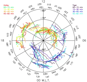
The format used to present the multi-beam SWB data in Fig. 7 was only useful for revealing large variations in SWB shape because the curves for different beams were superim-posed. Figure 8 reveals the detailed evolution of SWB shape for the Halley and TIGER radars during 08:00 to 22:00 UT on 1 April 2000. The SWBs were estimated using the C-F algorithm and a spectral width threshold of 150 m s−1. All
the points shown have been averaged over 15-min bins to re-duce clutter in the diagram, and then mapped to co-ordinates consisting of MLT and AACGM latitude. As explained in the caption, a different colour was used for results obtained in each 15-min bin past the hour. UT at Halley (H) and TIGER (T) are annotated around the perimeter. Keep in mind that these results do not show an instantaneous “snapshot” of SWB shape at all MLT. Rather, space and time variations are mixed because of the limited longitudinal coverage of both radars.
Fig. 8. SWBs for Halley and TIGER radar full scans during 08:00
to 22:00 UT on 1 April 2000. The results have been mapped to co-ordinates consisting of MLT and AACGM latitude. The SWBs have been averaged over 15-min intervals, and are color coded as follows: Halley 00–15 min (green), 15–30 min (yellow), 30– 45 min (orange), and 45–60 min (red) past the hour, and TIGER 00–15 min (black), 15–30 min (purple), 30–45 min (blue), and 45– 60 min (aqua) past the hour.
Figure 9 represents an alternative method of portraying relative variations in SWB shape. For brevity, only the more subtle variations measured by the Halley radar are shown. For each 5-min interval, the magnetic latitude of the SWB identified on each beam was averaged. Up to 16 averages were then available to calculate the average magnetic latitude of the SWB across the entire FOV. The calculations were per-formed in this way to prevent the high-time resolution beam 8 results biasing the results. Next, the difference between the average latitude of the SWB for each beam and the average latitude of the SWB across the entire FOV was calculated. These are the numbers colour coded in Fig. 9.
The way the differences in Fig. 9 change with beam num-ber indicates the “instantaneous” shape of the SWB, assum-ing it was stationary durassum-ing the 5-min averagassum-ing time. Note that if the SWB forms a spatial bay extending to higher lati-tudes in the radar FOV, the differences will be negative (cold colours) on the central beams and positive (warm colours) on the eastern and western-most beams. Conversely, if the SWB forms a spatial bulge extending to lower latitudes, the differences will be positive on the central beams, and nega-tive towards the edge beams.
It would be impractical to explain all of the numerous, complicated spatial and temporal fluctuations in Figs. 8 and 9. Keeping in mind that the colour key in Fig. 9 ranges over ∼3◦3, only the largest variations are summarised as follows: The locus of curves in Fig. 8 reveals that the Halley dayside SWB had an equatorward tilt toward the east at
Fig. 9. SWB shape versus UT for the Halley radar during 08:00
to 18:00 UT, 1 April 2000. The colour scale gives the difference between the magnetic latitude of the SWB on each beam versus the average magnetic latitude of the SWB across all beams. The calculations were performed at 5-min intervals. See the text for further explanation.
dawn (∼06:00 MLT), and a subsequent poleward tilt to-ward the east beyond ∼09:00 MLT. Hence, there was an apparent equatorward bulge during these quiet, Bynegative
conditions. In the 10:00 to 14:00 MLT sector (i.e. noon) the variations in SWB shape were complicated, with evi-dence for equatorward bulges in some scans (Fig. 9; 13:45 to 14:00 UT), and poleward bays in others (15:45 to 16:15 UT). Perhaps these alternating bulges and bays were somehow re-lated to magnetic reconnection occurring under Bznorthward
conditions (cf. Chisham et al., 2001; Pinnock and Rodger, 2001).
Figure 9 facilitates a more accurate timing of these changes in Halley SWB shape. During ∼08:00 to 10:35 UT the SWB had an equatorward tilt toward the east. Then, dur-ing ∼10:55 to 13:05 UT an equatorward tilt toward the west emerged. Again, there was a distinct equatorward tilt toward the west during ∼14:20 to 15:45 UT, preceding the forma-tion of a transient poleward bay during 15:45 to 16:20 UT
(the green curve near noon in Fig. 8). During ∼16:20 to 17:15 UT, the SWB had a strong equatorward bulge toward the east in the post-noon sector under Bzstrongly southward,
Bynegative conditions.
During the remainder of the study interval, there were many fluctuations in SWB shape, but it was approximately L-shell aligned during 18:00 to 19:40 UT (∼16:00 MLT) when Bzwas trending northward again.
Figure 8, and the equivalent of Fig. 9 for TIGER revealed the detailed behaviour of the nightside SWB:
From 08:55 to 11:40 UT (∼19:00 to 02:00 MLT) there was a large, distinct variation in the SWB location with beam number (cf. Fig. 7a). In the pre-midnight sector, the SWB was tilted poleward towards the west, and equatorward to-wards the east. The SWB evolved from a true SWB to a group delay aligned scatter boundary just prior to 11:40 UT. During 11:45 to 13:40 UT (∼22:00 to 04:00 MLT) the SWB shape was initially magnetic L-shell aligned to first order. However, the SWB shape developed a significant equator-ward tilt toequator-ward the east post midnight, during 13:45 to 16:10 UT. This equatorward tilt was stronger on the eastern-most beams from the start of the recovery phase of the first minor substorm (13:32 UT).
A second substorm caused the loss of ionospheric scat-ter during ∼16:50 to 19:20 UT. When scatscat-ter subsequently returned near dawn, the TIGER SWB was initially located slightly equatorward toward the east. Otherwise, there was no striking SWB shape near dawn.
In summary, the preceding analysis illustrates the potential of SuperDARN to reveal ongoing variability in the shape of the SWB, and thus at times, perhaps also the OCB.
4 Discussion and interpretation
4.1 Substorm-related changes in the spectral width bound-ary
First, we interpret the observed behaviour of the dayside SWB in the context of the expanding/contracting model of high-latitude convection, and discuss the way in which the behaviour of the nightside SWB is organized according to substorm phase.
Here the onset of the first, small substorm (−122 nT) oc-curred at 13:17 UT (Fig. 2e), near to when the Bzcomponent
swung northward after Bz was ∼−3 nT for ∼1 h (Fig. 2c).
The Halley radar measured an ∼4◦3equatorward
expan-sion of the dayside SWB throughout the substorm growth and expansion phases (Figs. 3a and 4a). The Halley day-side response was more obvious when “sea echoes” were used in the C-F algorithm (i.e. some of these echoes were actually from the ionosphere). The TIGER radar also mea-sured an ∼3◦3equatorward expansion of the SWB during the growth, expansion, and recovery phases (Figs. 3b and 4c). This equatorward expansion was delayed by several tens of minutes after that observed by the Halley radar. The TIGER radar measured a rapid poleward contraction of the nightside
SWB at 14:00 UT during the recovery phase of the first sub-storm. Perhaps the dayside SWB measured by Halley con-tracted simultaneously, or shortly after, but the absence of echoes detected by Halley makes this difficult to tell.
The growth phase of the second moderate substorm (−413 nT) began near 15:25 UT, the arrival time of a major, step-like Bz southward transition (Parkinson et al., 2002c).
Expansion onset occurred at 16:51 UT when Bzwas
gradu-ally swinging further southward, and the start of the recovery phase, 17:56 UT, may have been coincident with the arrival of a Bz northward spike. Bz continued to trend northward
during the remainder of the recovery phase, and beyond. The Halley line-of-sight velocity data revealed an unam-biguous response of the noon-sector ionosphere to the Bz
southward transition at 15:25 UT (Parkinson et al., 2002c). However, depending on the algorithm used to estimate the nightside SWB, the TIGER observations did not show it ex-panding equatorward until 15:35 UT. This time delay may represent the point beyond which the effects of enhanced dayside reconnection superceded the effects of magnetotail reconnection within the nightside ionosphere. Such obser-vations must be understood in the context of detailed mod-eling of magnetospheric processes, including dayside recon-nection and substorm-related activity.
The Halley radar initially observed a band of scatter con-tracting poleward at 15:25 UT. However, an enlargement of Fig. 3a shows that scatter with low power began to expand equatorward at the same time. This bifurcation resembles the radar and auroral imager signatures presented by Milan et al. (2000) for a similar Bz southward transition. Overall,
the Halley scatter underwent a dramatic equatorward expan-sion from −81◦3at 15:25 UT to −67.5◦3at 18:35 UT, before contracting poleward beyond this time. The rapid ex-pansion of the dayside polar cap ionosphere (∼4.7◦3h−1) was probably caused by the accumulation of open magnetic flux generated by intense dayside merging. The nightside reconnection rate must have been slower than the dayside re-connection rate until 18:35 UT.
The behaviour of the dayside SWB during the second moderate substorm was similar to that during the first mi-nor substorm, namely an equatorward expansion during the growth and expansion phases of the substorm, followed by a poleward contraction during the recovery phase. The TIGER observations suggest that the response of the nightside SWB was similar, except that the equatorward expansion was de-layed during the growth and expansion phases. The night-side SWB expanded equatorward during the growth phase until 16:51 UT when most ionospheric scatter was lost. It is probable that the SWB continued to expand further equator-ward after 16:51 UT, and then rapidly contracted poleequator-ward sometime during the recovery phase, 17:57 to 19:20 UT. If the close range scatter observed during 17:20 to 18:40 UT (Figs. 3b and 4c) represented the peak equatorward expan-sion of the SWB, it implies that the poleward contraction of the nightside SWB was more rapid than the preceding con-traction of the dayside SWB.
The previous interpretation is supported by the results of Parkinson et al. (2003b)1. They investigated how well the nightside SWB agreed with the poleward edge of the auro-ral oval during two nights which encompassed 4 substorms. During 3 of the substorms, the SWB was observed to grad-ually expand equatorward during the expansion phase, and then rapidly contract poleward during the recovery phase. For the remaining small substorm, Bzwas weakly southward,
and the post-midnight SWB was trending poleward before and during the substorm.
The behaviour of the nightside SWB during substorms, es-pecially the rapid poleward contractions, may represent the time when the effects of nightside reconnection superceded the effects of dayside reconnection. However, the behaviour may also be related to the dynamics of particle precipitation during substorms. For example, the aurora are well known to rapidly expand poleward at expansion onset in the post-midnight sector. These poleward aurora migrate to earlier MLT, a phenomenon known as “westward traveling surge”. Perhaps the rapid poleward contractions of the pre-midnight SWB are caused by the arrival of hot particle precipitation initiated somewhat earlier. This idea will be tested when co-incident global satellite observations of auroral emissions be-come available.
The preceding observations suggest that the behaviour of the radar SWBs were closely related to expansions and con-tractions of the OCB in response to the combined effects of changing day- and nightside reconnection rates, including substorm processes. It seems that the radar SWB behaves in a similar way to the OCB in many MLT sectors, and for various levels of geomagnetic activity. However, our obser-vations suggest that the SWB is often a better proxy for the poleward limit of hot particle precipitation (e.g. Fig. 7 and others not shown).
4.2 Formation of the spectral width boundary
Previous studies have shown the nightside SWB is often co-incident with the OCB (Lester et al., 2001; Parkinson et al., 2002b, 2003b1; Chisham et al., 2004), and often behaves in a similar way, but it is clearly a different entity. The work of Woodfield et al. (2002a, b, c) suggests that the nightside SWB is often found equatorward of the OCB in the post-midnight sector, and the results of Parkinson et al. (2003b)1 support this view. The present results (i.e. Fig. 7a) also im-ply that the SWB can be found equatorward of the OCB in the pre-midnight sector, as well as the post-midnight sector. What then, causes the formation of a SWB?
Whilst not the focus of this study, we first briefly consider the possible drivers of the electric field fluctuations caus-ing the large spectral widths. Large-scale variations in the convection pattern cannot account for the very large spectral widths often observed by SuperDARN radars (Andr´e et al., 2000b). The large spectral widths are thought to be caused by electric field variations carried by ULF waves in the Pc 1-2 frequency range (Andr´e et al., 1999, 2000a), or short-scale electric fields radiating from filamentary field-aligned
currents (Huber and Sofko, 2000). This implies SWBs may form in proximity to the OCB and elsewhere because of spa-tial and temporal variations in the activity of the spectral width drivers. However, spatial and temporal variations in the properties of the ionosphere may also contribute to the formation of SWBs.
It is well known that polarization effects enhance (sup-press) electric fields in regions of low (high) height-integrated Pedersen conductivity (Pedersen conductance). Whilst not definitive, Fig. 7 and previously published re-sults actually suggest that the nightside SWB is often a better proxy for the poleward limit of hot electron and ion precip-itation, ∼1 keV and 10 keV, respectively (diamonds). This suggests that variations in E-region conductivity may play an important role in the formation of the SWB. The short-scale electric field fluctuations which cause the large spectral widths observed in the polar cap ionosphere must be shorted-out or suppressed by the very large Pedersen conductance, 6p∼10 mhos, occurring in the nightside auroral oval. There
is a theoretical basis, supported by measurements, for this hypothesis.
Weimer et al. (1985) analysed auroral field-perpendicular electric field measurements made by the Dynamics Explorer 1 (DE 1) spacecraft at high altitude, coincident with simi-lar measurements made by the DE 2 spacecraft at low alti-tude. First, a magnetic dipole model was used to map the electric field strengths measured by the two spacecraft to the same height. Next, the electric field fluctuations were Fourier analysed during intervals when the measurements were made on nearly the same magnetic field lines. Similar large-scale (>100 km) electric field fluctuations were transmitted from high altitude to low latitude in and outside the auroral oval. However, within the auroral oval, the small-scale (<100 km) electric field fluctuations were suppressed at low altitude. This was mathematically consistent with the requirement of field-parallel potential drops and currents above auroral arcs of width <100 km.
Based on theory given by Lyons (1980, 1981) and Chiu et al. (1981), Weimer et al. derived an important equation describing the suppression of the low-altitude, ionospheric electric field Eixwith respect to the high-altitude, equatorial electric field Ehx. Re-organising their Eq. (24), we obtain
Exi =a/(a + 6pk2) Exh, (1)
where a is the finite parallel conductance, and k is the wave number in the field-perpendicular direction. For large wave-lengths, k2→0, and Ei
x=Ehx. For short wavelengths, Exi/Exh
decreases as 1/k2. For 6p=0, all small-scale fluctuations are
transmitted to the ionosphere, but as 6p increases, only the
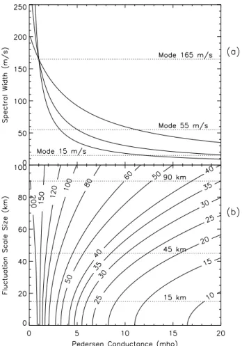
large-scale fluctuations are transmitted. Because the small-scale fluctuations drive the field-perpendicular plasma mo-tions causing the radar spectral widths, a SWB should form where there is a significant change in Pedersen conductance. In fact, we can use the theory given in Weimer et al. to model the changes in nightside spectral widths shown in Figs. 3 and 6. Figure 5 showed that the mode (most probable)
values of the three spectral width distributions were ∼15, 55, and 165 m s−1. We will show that the spectral width
dis-tributions with smaller mode values observed in the auroral oval can be explained solely by the Pedersen conductance suppressing the electric field fluctuations, as opposed to a re-duction in the activity of the electric field fluctuation driver. However, we actually expect both factors to play a role.
First, we note that because v=E/B, Eq. (1) can also be used to map the magnitudes of the velocity fluctuations, 1v, corresponding to the electric field fluctuations. Next, we as-sume that the radar measurement process is linear, so that the observed spectral widths are given, to first order, by the mag-nitude of the velocity fluctuations throughout the observation cells (see Ponomarenko and Waters, 2003), i.e. the spectral widths are approximately determined by ∼1v at the spatial scales most likely to affect the observations. However, this is only an approximation because velocity fluctuations exist in both space and time. Nevertheless, the velocity fluctuations which do occur must still be given by ∼1v.
The size of the observation cells at the ranges where most F-region ionospheric scatter is observed is of the order of 45 km by 100 km (i.e. the pulse width by the beam width). Although we will consider the effects of velocity fluctuations at all plausible scales affecting the observation cells, initially we only consider the effects of wave numbers k correspond-ing to fluctuation scale sizes of 15, 45, and 90 km. These and nearby fluctuation scale sizes will strongly affect the radar spectral widths.
We will assume that the spectral width distribution with a mode value of ∼165 m s−1 occurs in the polar cap iono-sphere where 6p=1 mho. This initial choice is plausible
given that 6p is often ∼0.5 to 2 mho in the dark polar
cap. Next, the free parameter a can be varied widely, but a=2×10⁻⁸mho m−2 is consistent with the observations given in Weimer et al. (more on these choices later). Apply-ing Eq. (1), we calculate the magnitude of the velocity fluc-tuations in the magnetosphere corresponding to the veloc-ity fluctuations in the ionosphere for different spatial wave numbers k. The velocity fluctuations in the magnetosphere (mapped to the common ionospheric altitude) are 205, 326, 1613 m s−1for fluctuation scale sizes of 15, 45, and 90 km, respectively. For example, this means that velocity fluctu-ations of 326 m s−1 in the magnetosphere map to velocity fluctuations of 165 m s−1in the polar cap ionosphere, at scale size 45 km.
Having calculated the magnitude of the velocity fluctua-tions in the magnetosphere for various scale sizes, we now calculate what these values map to in the auroral ionosphere where the Pedersen conductance may be enhanced by ener-getic particle precipitation. We sort these results according to fluctuation scale size. Figure 10a shows the results for scale sizes of 15 km (bottom curve), 45 km (middle curve), and 90 km (top curve). Note that all three curves cross at the point where 6p=1 mho and 1v=165 m s−1. If the
spec-tral widths were entirely due to velocity fluctuations of scale size 15 km, then the population of spectral widths with mode value 55 m s−1can be explained by a Pedersen conductance
of 3 mho, whereas the population with mode value 15 m s−1
can be explained by a Pedersen conductance of 12 mho. If we consider a fluctuation scale size of 45 km, then these con-ductances increase to 5 and 20 mho, respectively. However, the conductances become implausibly large for scale sizes of 90 km.
Figure 10b show the same calculations as in Fig. 10a, ex-cept the contours show the ionospheric spectral widths for all fluctuation scale sizes. Again, the auroral spectral width distributions with mode values of 55 and 15 m s−1 are best explained by fluctuation scale sizes of 45 km and less, and plausible Pedersen conductances of 5 to 20 mho. At larger scale sizes, unusually large values of Pedersen conductance must be invoked. Hence, our calculations are consistent with the notion that large SuperDARN spectral widths are caused by ∼10-km scale size vortices generated by filamentary par-allel currents (Huber and Sofko, 2000).
All of the curves in Fig. 10 change with our choice of a or 6p in the polar cap ionosphere. For example,
increas-ing 6p in the polar cap to 2 mho means that more
conduc-tance is required to explain the auroral spectral widths, and thus only ∼10-km scale vortices can explain the observed spectral widths. Similarly, increasing the free parameter a to 2×10⁻⁷mho m−2 means that more conductance is re-quired to explain the auroral spectral widths, and again, only ∼10-km scale vortices offer a viable explanation. However, decreasing a to 2×10⁻⁹mho m−2means that even 100-km scale size vortices can explain the observed spectral widths for plausible values of auroral conductance. Of course, the finite parallel conductance might be larger in the polar cap, and smaller in the auroral oval, but making this change does not change our conclusions.
Our first-order model shows the observed changes in the nightside spectral widths are consistent with the suppression of the electric field fluctuations by Pedersen conductance enhanced by particle-precipitation. However, our modeling does not exclude the possibility of ULF waves in the Pc 1-2 frequency range contributing to the generation of moderate spectral widths, as modeled by Andr´e et al. A future goal will be to simulate the complete spectral width distributions (e.g. Fig. 5) using a spectral width simulator similar to that of Andr´e et al., but incorporating the effects of ULF waves and spatio-temporal velocity fluctuations consistent with the Weimer et al. theory. Modeling is also required to estab-lish whether the reflection coefficient of ULF waves becomes large for a highly conducting E-region. Depending on the wave mode, perhaps the electric field fluctuations carried by the incident and reflected waves are suppressed by enhanced ionospheric conductivity.
The preceding explanation of the SWB is consistent with the results of earlier studies. Dudeney et al. (1998), Fig. 3, suggests that as the energy and flux of precipitating particles (i.e. Pedersen conductance) increases, the amplitude of high frequency electric field fluctuations decreases, as well as the radar spectral widths. This is direct observational support for our hypothesis that the radar spectral widths are suppressed in regions of enhanced Pedersen conductance.
Fig. 10. (a) The three curves show the variation of the
spec-tral width with Pedersen conductance for velocity fluctuations on spatial scales of 15 km (bottom curve), 45 km (middle curve), and 90 km (top curve). The calculations assume a most proba-ble spectral width of 165 m s−1in the polar cap ionosphere where a=2×10⁻⁸mho m−2and 6p=1 mho, (b) The same calculations as
in (a), except the contours show the spectral width versus Pedersen conductance for all auroral fluctuation scale sizes between zero and 100 km.
Lester et al. (2001) and Parkinson et al. (2002b, 2003b1) reported DMSP poleward edges in agreement with the night-side radar SWB. In these studies, the hot particle precipita-tion tended to extend close to the poleward edge of the au-roral oval. Parkinson et al. (2003b)1 found that the OCB was less likely to agree with the SWB in the morning sec-tor when colder precipitation extended poleward of the hot particle zone, i.e. again, the SWB was probably more closely aligned with the poleward edge of hot particle precipitation.
Parkinson et al. (2002b) showed that the large-scale veloc-ities (electric fields) tend to rapidly decay across the night-side SWB, becoming slower and more laminar in the au-roral oval. Again, this suggests that the small-scale turbu-lence observed by spacecraft within the plasma sheet does not completely map to the highly conducting auroral iono-sphere. These observations are also consistent with the im-portant role of Pedersen conductivity in the formation of the SWB.