Technical note: The libRadtran software package for radiative transfer calculations ? description and examples of use

(1)

HAL Id: hal-00303886

https://hal.archives-ouvertes.fr/hal-00303886

Submitted on 9 Mar 2005

HAL is a multi-disciplinary open access

archive for the deposit and dissemination of sci-entific research documents, whether they are pub-lished or not. The documents may come from teaching and research institutions in France or abroad, or from public or private research centers.

L’archive ouverte pluridisciplinaire HAL, est destinée au dépôt et à la diffusion de documents scientifiques de niveau recherche, publiés ou non, émanant des établissements d’enseignement et de recherche français ou étrangers, des laboratoires publics ou privés.

Technical note: The libRadtran software package for

radiative transfer calculations ? description and

examples of use

B. Mayer, A. Kylling

To cite this version:

B. Mayer, A. Kylling. Technical note: The libRadtran software package for radiative transfer calcula-tions ? description and examples of use. Atmospheric Chemistry and Physics Discussions, European Geosciences Union, 2005, 5 (2), pp.1319-1381. �hal-00303886�

(2)

ACPD

5, 1319–1381, 2005

The

libRadtran radiative transfer package

B. Mayer and A. Kylling

Title Page Abstract Introduction Conclusions References Tables Figures J I J I Back Close Full Screen / Esc

Print Version Interactive Discussion

EGU

Atmos. Chem. Phys. Discuss., 5, 1319–1381, 2005 www.atmos-chem-phys.org/acpd/5/1319/

SRef-ID: 1680-7375/acpd/2005-5-1319 European Geosciences Union

Atmospheric Chemistry and Physics Discussions

Technical note: The libRadtran software

package for radiative transfer calculations

– description and examples of use

B. Mayer1and A. Kylling2,3

1

Deutsches Zentrum f ür Luft- und Raumfahrt (DLR), Institut f ür Physik der Atmosph äre, Oberpfaffenhofen, Germany

2

St. Olavs Hospital, Trondheim University Hospital, Norway

3

previously at: Norwegian Institute for Air Research (NILU), Kjeller, Norway

Received: 25 November 2004 – Accepted: 30 December 2004 – Published: 9 March 2005 Correspondence to: B. Mayer (bernhard.mayer@dlr.de)

(3)

ACPD

5, 1319–1381, 2005

The

EGU

Abstract

The libRadtran software package is a suite of tools for radiative transfer calculations in the Earth’s atmosphere. Its main tool is the uvspec program. It may be used to compute radiances, irradiances and actinic fluxes in the solar and terrestrial part of the spectrum. The design of uvspec allows simple problems to be easily solved using

5

defaults and included data, hence making it suitable for educational purposes. At the same time the flexibility in how and what input may be specified makes it a powerful and versatile tool for research tasks. The uvspec tool and additional tools included with libRadtran are described and realistic examples of their use are given. The libRad-tran software package is available fromhttp://www.libradtran.org.

10

1. Introduction

To understand the Earth system, knowledge about the solar and terrestrial radiation environment is required. Radiative transfer models are used to calculate the radiation field for given atmospheric and surface conditions. Applications for radiative transfer calculations include remote sensing, process studies, UV-forecast, radiative forcing,

15

photolysis frequencies, radiative heating/cooling etc. Flexible and versatile tools are required to realistically handle the variety of problems. Here the libRadtran software package for radiative transfer calculations in the Earth’s atmosphere is described. The libRadtran package includes numerous tools that may be used to address various prob-lems related to atmospheric radiation. The main tool is the uvspec radiative transfer

20

model. It will be described first. Secondly, the other libRadtran tools will be summa-rized followed by examples of usage of the various tools. The description applies to version 1.0 or later of the package.

(4)

ACPD

5, 1319–1381, 2005

The

EGU

2. The uvspec radiative transfer model

The uvspec radiative transfer model calculates the radiation field in the Earth’s atmo-sphere for a variety of atmospheric conditions. Originally it was designed to calculate spectral irradiance in the ultraviolet and visible parts of the spectrum. Over the years, uvspec has undergone numerous extensions and improvements, including a complete

5

rewrite in 1997 since when the model package has been called libRadtran. Probably the most important change was an extension from the ultraviolet to the complete solar and thermal spectral ranges. The name uvspec is thus outdated, but has been kept for historical reasons. Thus, uvspec still is the name of the radiative transfer model while libRadtran refers to the complete software package including data sets, tools,

10

examples, and documentation.

The uvspec model is invoked from the command line (similar both for UNIX-like and Windows types of operating systems)

uvspec < input file > output file

where the input file is a free format ASCII file that contains options and corresponding

15

parameters specified by the user. A description of the numerous options (close to 200 for version 1.0) and respective parameters is provided in the libRadtran User’s Guide. Some options are described below. They are identified by being written in bold face, for example quiet which takes no parameters and turns off output of a number

of informative but not neccessarily required messages, anddens column O3 340.0 20

DU which takes three parameters and scales the ozone column to 340 Dobson units in

this example. The format of the output file differs depending on the choosen radiative transfer equation solver and the output options specified by the user. The output always includes the direct and diffuse downward, and the diffuse upward irradiances. Actinic flux and radiances for arbitrary angles may be requested by the user. A complete

25

description is given in the libRadtran User’s Guide.

A unique feature of uvspec is that the user has a choice of various radiative transfer equation solvers which are selected by therte solver option in the input file. This way,

(5)

ACPD

5, 1319–1381, 2005

The

EGU

for the radiative transfer problem at hand an appropriate solver may be chosen, e.g., a fast two-stream code to calculate approximate irradiance, or a discrete ordinate code to accurately simulate radiances, with or without polarization. Details about the solvers are given below.

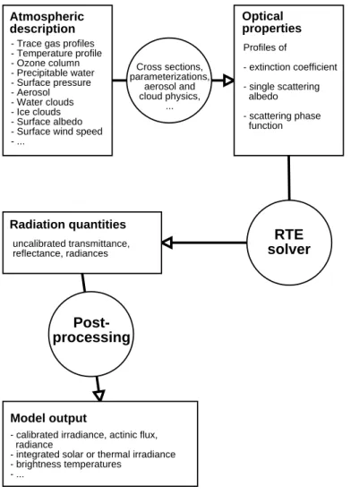
The uvspec model includes the following three essential parts: (1) An atmospheric

5

shell which converts atmospheric properties like ozone profile, surface pressure, or cloud microphysical parameters into optical properties required as input to (2) the ra-diative transfer equation solver which calculates radiances, irradiances, and actinic fluxes for the given optical properties; finally (3) post-processing of the solver output including multiplication with the extraterrestrial solar irradiance, correction of Earth-Sun

10

distance, convolution with a slit function, or integration over wavelength (depending on the choice of the user). For an overview see Fig.1. The components are described in the following.

2.1. Radiative transfer equation solvers

At the heart of all radiative transfer models is a procedure to calculate the radiation

15

field for a given distribution of optical properties. This procedure ranges from a variety of parameterizations and approximations to sophisticated and accurate solutions of the full three-dimensional radiative transfer equation. The radiative transfer equation may be written as (Chandrasekhar,1960;Thomas and Stamnes,1999)

d L

βd s = −L + J, (1)

20

where the source function J is defined as

J= ω

4π Z

p(Ω, Ω0)L(Ω0)dΩ0+ (1 − ω)B(T ). (2)

Here L is the radiance at location (x, y, z), β the volume extinction coefficient, ω the single scattering albedo, p(Ω, Ω0) the phase function giving the likelihood of a scattering

(6)

ACPD

5, 1319–1381, 2005

The

EGU

event redistributing radiation from directionΩ0toΩ, and B(T ) the Planck function. The latter can usually be neglected for wavelengths below about 4 µm. Numerous methods exist to solve Eq. (1). The problem at hand sets conditions that must be satisfied when solving the radiative transfer equation.

As opposed to most other radiative transfer models, uvspec is not based on a single

5

method to solve Eq. (1) but rather includes a number of different radiative transfer equation solvers (Table1).

Thus, given a problem, the user may easily choose the appropriate solver. Once the radiative transfer equation is solved a number of radiative quantities are calculated. These include the downward direct and diffuse E↓ irradiances and the upward E_↑

irra-10 diance: E_↓= Z 2π L(Ω) cos θdΩ =Z2π 0 Zπ/2 0 L(θ, φ) cos θ sin θd θd φ (3) E_↑= Z2π 0 Z0 −π/2 L(θ, φ) cos θ sin θd θd φ (4)

and the corresponding actinic fluxes

15 F_↓= Z 2π L(Ω)dΩ =Z2π 0 Zπ/2 0 L(θ, φ) sin θd θd φ (5) F_↑= Z2π 0 Z0 −π/2 L(θ, φ) sin θd θd φ. (6)

Here θ and φ are the polar and azimuth angles, respectively. Other quantities may also be calculated, see Table1and the examples in Sect.4.

(7)

ACPD

5, 1319–1381, 2005

The

EGU

The radiation quantities in Eqs. (1–6) are scalar. The corresponding full vector radi-ation quantities are calculated if the POLRADTRAN solver is invoked which accounts for polarization. Most of the solvers are plane-parallel (PP), that is, they neglect the Earth’s curvature and assume an atmosphere of parallel homogeneous layers. This is generally a good assumption for solar and observation zenith angles smaller than about

5

70◦ (Dahlback and Stamnes,1991). Some of the solvers include a so-called

pseudo-spherical (PS) correction which treats the direct solar beam in pseudo-spherical geometry and the multiple scattering in plane-parallel approximation (Dahlback and Stamnes,1991). These usually provide a reasonable solution for low sun. For low observation angles (e.g. for limb scan geometry), however, the pseudo-spherical correction does not

im-10

prove the result. Here, a fully-spherical solver is required which is currently not provided by uvspec. Also, the three-dimensional MYSTIC (Monte Carlo code for the physically correct tracing of photons in cloudy atmospheres) solver (Mayer, 1999,2000), men-tioned in Table1, is not included in the libRadtran distribution. Due to the complexity of three-dimensional problems we prefer to solve those in close collaboration and

inter-15

ested groups are therefore invited to contact Bernhard Mayer. 2.2. Spectral resolution

The spectral resolution may be treated in four different ways by uvspec. The spectrally resolved calculation and the line-by-line calculation are more or less exact methods. The correlated-k distribution and the pseudo-spectral calculation are approximations

20

that provide a compromise between speed and accuracy. In the following the four methods are described including a discussion of the applicability for a specific purpose. 2.2.1. Spectrally resolved calculation

A spectrally resolved calculation is the most straightforward way, and will be the choice for most users interested in the ultraviolet and visible spectral ranges. In the UV and

25

(8)

ACPD

5, 1319–1381, 2005

The

EGU

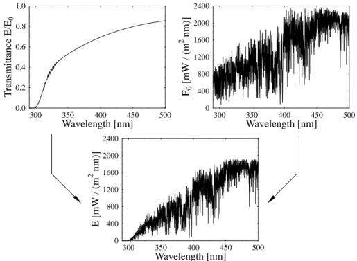
the most important of these being the Hartley, Huggins, and Chappuis bands of ozone. Hence, a radiative transfer calculation with 0.5 nm steps below 350 nm and 1 nm steps above 350 nm is sufficient for most applications. On the other hand, the solar spectrum is highly variable with wavelength, due to the Fraunhofer lines. The general idea was therefore to calculate the atmospheric transmission with moderate resolution,

interpo-5

late to the high resolution of the extraterrestrial irradiance, and multiply both. Figure2

gives an example of this method.

Absorption cross sections for various species are included in uvspec, see Table 2. However, this method is only applicable in the ultraviolet and parts of the visible spec-trum. At longer wavelengths the atmospheric transmittance is highly variable with

10

wavelength, due to the narrow rotation-vibration lines of various species. For spectrally resolved calculations the water vapour and oxygen absorption bands are not included, thus this approach is certainly not applicable above 800 nm. See further discussion in Sect.2.3.1. Spectrally resolved calculations are the default in uvspec.

2.2.2. Line-by-line calculation

15

In the infrared, molecular absorption spectra are characterized by thousands of nar-row absorption lines. There are two ways to treat these, either by highly resolved spectral calculations, so-called line-by-line calculations, or by a band parameteriza-tion. Concerning line-by-line, uvspec offers the possibility to define a spectrally re-solved absorption cross section profile using molecular tau file. There is no option 20

in libRadtran to generate such amolecular tau file, because (1) the high resolution

transmission molecular absorption database (http://www.hitran.com) which forms the basis for such calculations amounts to about 100 MByte which are updated continu-ously; and (2), there are sophisticated line-by-line programs available, like e.g. genln2

(Edwards,1992). Using genln2 it is straightforward to create molecular absorption

pro-25

files for uvspec line-by-line calculations. Figure 3shows an example of a line-by-line calculation of the atmospheric transmittance in two selected solar and thermal spec-tral ranges, the O₂A absorption band around 760 nm and a region within the infrared

(9)

ACPD

5, 1319–1381, 2005

The

EGU

atmospheric window around 10 µm.

All spectral lines in the left figure are due to absorption by oxygen, while the ones in the right figure are due to ozone, water vapour, and carbon dioxide. Line-by-line calculations are obviously the most accurate but also the most time-consuming way to make radiation calculations.

5

2.2.3. Correlated-k and pseudo-spectral calculations

For most applications, however, line-by-line calculations are far too slow. Here one needs a band parameterization, and the most accurate of these is the so-called correlated-k approximation (Lacis and Oinas, 1991; Yang et al., 2000). Several correlated-k parameterizations have been implemented in uvspec. These are invoked

10

with the optioncorrelated k followed by one of the following:

kato. The parameterization by Kato et al. (1999). It covers the solar spectral range and includes 575 subbands, that is, 575 calls to therte solver. The absorption

coefficients are based on HITRAN 1992.

15

kato2. A new, optimized version of the above tables (Seiji Kato, private com-munication 2003), with only 148 subbands (that is, calls to the rte solver). The uncertainty is only slightly higher thankato. The absorption coefficients are based on

HITRAN 2000.

20

fu. The Fu and Liou (1992) is a fast parameterization developed for climate

models. It covers both the solar shortwave and the terrestrial longwave.

avhrr kratz. The Kratz and Varanasi (1995) parameterization covers the

Ad-25

vanced Very High Resolution Radiometer (AVHRR) instrument channels which are calculated as a linear combination of the bands output by uvspec.

(10)

ACPD

5, 1319–1381, 2005

The

EGU

lowtran. The lowtran option is actually not a real correlated-k

parameteriza-tion, but allows pseudo-spectral calculations covering the whole spectral range. It has been adopted from the SBDART radiative transfer model (Ricchiazzi et al.,1998) from which we quote

SBDART relies on low-resolution band models developed for the LOWTRAN

5

7 atmospheric transmission code (Pierluissi and Peng,1985). These mod-els provide clear-sky atmospheric transmission from 0 to 50 000 cm−1 and include the effects of all radiatively active molecular species found in the Earth s atmosphere. The models are derived from detailed line-by-line cal-culations that are degraded to 20 cm−1resolution for use in LOWTRAN. This

10

translates to a wavelength resolution of about 5 nm in the visible and about 200 nm in the thermal infrared. These band models represent rather large wavelength bands, and the transmission functions do not necessarily follow Beers Law. This means that the fractional transmission through a slab of material depends not only on the slab thickness, but also on the amount

15

of material penetrated before entering the slab. Since the radiative transfer equation solved by SBDART assumes Beers Law behavior, it is necessary to express the transmission as the sum of several exponential functions (

Wis-combe and Evans,1977). SBDART uses a three-term exponential fit, which was also obtained from LOWTRAN 7. Each term in the exponential fit

im-20

plies a separate solution of the radiation transfer equation. Hence, the RT equation solver only needs to be invoked three times for each spectral incre-ment. This is a great computational economy compared to a higher order fitting polynomial, but it may also be a source of significant error.

user specified. Allows a user-defined correlated-k parameterization for a specific at-25

mospheric profile.

For more information on these parameterizations please refer to the libRadtran docu-mentation and the referenced publications. Correlated-k is a powerful way to calculate spectrally integrated quantities, however, it takes away some flexibility. In particular this

(11)

ACPD

5, 1319–1381, 2005

The

EGU

implies that the wavelength grid is no longer chosen by the user but by the parameter-ization. The uvspec output is then no longer spectral quantities, e.g. W/(m2nm), but integrated over the spectral bands, e.g. W/m2. Note, however that this does not apply for thelowtran option which is still spectral.

2.3. Atmosphere

5

The uvspec model includes five classes of atmospheric constituents: Rayleigh scat-tering by air molecules, molecular absorption, aerosol, water and ice clouds. Each of those may be defined individually, using a variety of configuration options. The vertical resolution may be different for all components. Internally uvspec will merge the different vertical resolutions onto a common grid to be used by the radiative transfer equation

10

solver, thus giving the user total freedom when specifying the vertical profiles of the var-ious atmospheric constituents. Gaseous, aerosol, and ice cloud optical properties are considered one-dimensional and vary in the vertical only. For water clouds, a full three-dimensional input field may be specified to be used by either the MYSTIC solver or the independent pixel approximation (IPA) (see Sect.2.3.3). For each of the five classes,

15

either microphysical or optical properties may be defined by the user. E.g. molecular scattering is either defined by profiles of pressure and temperature or by explicitely specifying a profile of optical thickness; ice clouds may either be defined by their ice water content and particle properties (shape and size) or by explicitely defining pro-files of extinction coeffiecient, single scattering albedo, and scattering phase function.

20

Instead of defining complete profiles there is always the possibility to use standard pro-files and scale them with a columnar property, e.g. precipitable water, ozone column, or integrated aerosol optical thickness. This gives the user the flexibility to provide the model with whatever information is available and use standard assumptions for the unknown properties.

25

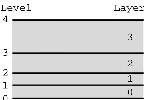
Please note that there are basically two ways of defining atmospheric properties as model input: at a given level, or for a given layer, see Fig.4.

(12)

ACPD

5, 1319–1381, 2005

The

EGU

defined at levels, as they are provided e.g. by radiosondes. A model layer, on the other hand, is an atmospheric layer defined by its bottom and top altitude. Some radiative transfer solvers like disort use the concept of layers, assuming that the optical prop-erties of the medium are constant within each layer. Some codes, like e.g. SHDOM

by Evans (1998) use the level concept and assume that the optical properties vary

5

linearly between levels. All RTE solvers within libRadtran use the layer concept. This has important implications for the interpretation of the input data: Profiles of pressure, temperature, trace gas concentrations etc. are interpreted as level properties, and in-terpolated linearly or logarithmically to obtain mean layer properties. Water and ice clouds may be either defined per level (default) or per layer. The layer concept is more

10

meaningful in this case because clouds usually have sharp boundaries. If optical prop-erties, like optical thickness, single scattering albedo, or the scattering phase function are defined as input, these usually refer to model layers, rather than levels. For most in-put parameters the assignment to level or layer is straightforward. In ambiguous cases, the manual and theverbose option will help to make correct decisions.

15

2.3.1. The molecular atmosphere

Profiles of pressure, temperature, and concentrations of ozone and optionally oxygen, water vapour, CO₂, and NO₂, defined in the atmosphere file form the starting point

for any uvspec calculation. These profiles may be specified in a number of ways, the simplest one being to use one of the included atmosphere files by Anderson et al.

20

(1986). For the various trace gases, vertical profiles may be specified in separate input files for each specie. Furthermore the vertical column of each specie may be scaled. To calculate the optical thickness from the concentration, absorption cross sections are needed. The trace gases currently considered by uvspec are listed in Table2including available choices for their cross sections.

25

As has been described in Sect.2.2, the definition of explicit spectral cross sections is only meaningful in the ultraviolet/visible where the absorption lines are broad enough to be covered explicitely with reasonable wavelength resolution. In the near and far

(13)

ACPD

5, 1319–1381, 2005

The

EGU

infrared regions, spectral lines are too dense so that an explicit (line-by-line) calculation is not feasible for most practical purposes. Table2gives an overview of the components included in the different approaches provided by uvspec.

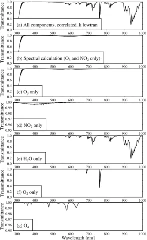
Figure 5 shows the atmospheric transmission in the ultraviolet/visible part of the spectrum and illustrates the contributions of individual components. The spectral

cal-5

culation includes only ozone and NO₂. It is clear that for wavelengths smaller than about 550 nm the spectral calculation is the method of choice, taking into account that this is by far the fastest method: only a single call to the radiative transfer solver is required per wavelength while for thecorrelated k options usually more than one call

is required; in the case of correlated k lowtran three calls to the radiative transfer 10

solver are required which leads to an about three-fold increase in computational time. Above 550 nm the uncertainty of the spectral calculation increases, due to the water vapour and oxygen absorption bands, and in the IR the spectral calculation obviously does not make any sense because there strong spectral absorption bands dominate the signal. For completeness, absorption by the O₄complex is included in the figure,

15

as parameterized in LOWTRAN/SBDART, see e.g.Pfeilsticker et al.(1997).

Molecular (Rayleigh) scattering is calculated from the density profile according to

Bodhaine et al.(1999). It can be modified e.g. bypressure 1013 which would set the

surface pressure to 1013 mbar and scale the profile accordingly. 2.3.2. Aerosols

20

Aerosols are tiny particles suspended in the air. They may originate from a variety of sources including volcanoes, dust storms, forest and grassland fires, living vege-tation, and sea spray as well as human activities such as the burning of fossil fuels and the alteration of natural surface cover. In consequence, aerosol properties are highly variable with location and time. Aerosol particles affect the radiation field by

25

absorption and scattering, depending on their origin. The high variability is reflected in the way aerosol is input to uvspec: Aerosols are specified in a hierarchical way. The most simple way to include aerosols is by the option aerosol default which will

(14)

ACPD

5, 1319–1381, 2005

The

EGU

include one of the aerosol models byShettle(1989) with the following properties: rural type aerosol in the boundary layer, background aerosol above 2 km, spring-summer conditions and a visibility of 50 km. These settings may be modified with the op-tionsaerosol haze, aerosol vulcan, aerosol season, and aerosol visibility. More

information can be introduced step by step, overwriting the default parameters. For

5

example,aerosol tau file, aerosol ssa file and aerosol gg file, can be used to

de-fine profiles of optical thickness, single scattering albedo, and asymmetry parameter. The integrated optical thickness can be set to a constant value usingaerosol set tau

or scaled with aerosol scale tau. The single scattering albedo may be scaled by aerosol scale ssa or set to a constant value by aerosol set ssa. The aerosol asym-10

metry factor may be set byaerosol set gg. The wavelength dependence of the aerosol

optical thickness may be specified using theaerosol angstrom option. For full

spec-ification of the aerosol scattering phase function theaerosol moments file option is

available. If microphysical properties are available these may be introduced by defin-ing the complex index of refraction aerosol refrac index or aerosol refrac file and 15

the size distributionaerosol sizedist file. Finally, one may define the aerosol optical

properties of each layer explicitely using aerosol files. This allows the user to

cal-culate aerosol optical properties with any single-scattering program and subsequently input these to uvspec. Full documentation of all aerosol options are included in the libRadtran documentation and some are used in the examples below. This example

20

demonstrates the general philosophy behind libRadtran: the starting point is always a standard model for a component which can be re-defined step-by-step by the user as data are available.

2.3.3. Clouds

Both water and ice clouds models are included in uvspec. The easiest way to include

25

a water or ice cloud is to specify vertical profiles of liquid or ice water content and effective droplet/particle radius. These properties may be defined either at model levels or per model layers. The microphysical properties of water clouds are converted to

(15)

ACPD

5, 1319–1381, 2005

The

EGU

optical properties either according to theHu and Stamnes(1993) parameterization or by Mie calculations. The latter are very time-consuming, hence they are not included as online calculations within uvspec. Rather there is an option to read in pre-calculated Mie tables which are available athttp://www.libradtran.org. These tables are provided for a set of 138 and 219 wavelengths between 250 nm and 100 µm for water and ice,

5

respectively. The wavelengths were chosen such that the linear interpolation of the extinction coefficient, single scattering albedo, and asymmetry parameter never deviate by more than 1% from the true value. For an overview of typical scattering phase functions for water clouds see Fig.6(top).

The main difference between water and ice clouds is that the latter usually consist

10

of non-spherical particles. Mie calculations for ice particles are only a first guess and certainly not a good approximation.

Hence, the conversion from microphysical to optical properties is less well-defined, and several parameterizations are available. The parameterizations byFu(1996) and

Fu et al.(1998) are suitable for calculation of irradiances. For radiances the

parame-15

terization ofKey et al.(2002) is available. Which parameterization to use is set by the optionic properties. For theKey et al.(2002) parameterizations the user may choose between six crystal habits. For an overview of typical scattering phase functions for ice clouds see Fig.6(bottom). The figure clearly shows that the parameterization by

Key et al.(2002) approximates the calculated phase function reasonably well. It is also

20

clear from the figure that ice particles should not be treated with Mie theory due to the large systematic difference particularly in the sideward direction.

As for the aerosol, there are several options to modify the optical properties of water and ice clouds. And of course there is also the option of defining all water and ice cloud properties explicitely using the optionswc files and ic files.

25

Clouds are complex three-dimensional distributions of water and ice particles. Full three-dimensional solvers like MYSTIC may handle realistic inhomogeneous clouds – usually for a high prize, consisting not only in a considerably higher computational cost, but even more important, the need to feed the model with realistic cloud structures. For

(16)

ACPD

5, 1319–1381, 2005

The

EGU

many applications, simpler approximations usually provide a reasonable alternative. The simplest clouds handled by radiative transfer equation solvers consist of homoge-neous layers which, however, is not necessarily a good assumption in general, see e.g.

Cahalan et al.(1994a,b);Scheirer and Macke (2003). One approach to approximate

horizontally inhomogeneous clouds with one-dimensional solvers is the independent

5

pixel approximation (IPA) (Cahalan et al.,1994b). The IPA ignores horizontal photon transport but includes horizontal inhomogeneities in the cloud optical properties. Even if nothing about the cloud structure is known, a simple approximation like handling only the cloudy part and the cloudless part of a scene with the independent pixel method (using only the cloud fraction as an extra parameter) is already a large improvement.

10

For many applications, clouds are and need to be treated plane-parallel, e.g. for remote sensing applications. Plane-parallel clouds are the default with uvspec. IPA calcula-tions may also readily be performed using the ic ipa files and wc ipa files options.

Examples of IPA calculations are shown below. 2.4. Surface

15

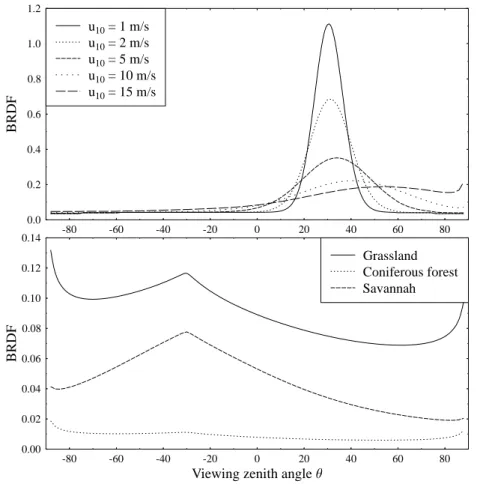
All the radiative transfer equation solvers in Table1may include a Lambertian reflecting lower surface. The albedo of this surface may be set to a constant value for all wave-lengths by thealbedo option or given wavelength dependent behaviour by the option albedo file. For the DISORT 2.0 and the MYSTIC solvers bidirectional reflectance

distribution functions (BRDF) for a variety of surfaces may be specified based on the

20

parameterization of Rahman et al. (1993). A parameterization of the BRDF of water surfaces is also included which depends mainly on wind speed and to a lower degree on plankton concentration and salinity. In contrast to the vegetation where the typical hot spot occurs in the 180◦ backscatter direction, here the main feature is specular reflection. The parameterization in uvspec was adopted from the 6S code (Vermote

25

et al.,1997) and is based on the measurements ofCox and Munk(1954a,b) and the calculations ofNakajima and Tanaka(1983). Figure7shows examples of the BRDF of land and water surfaces, as parameterized in uvspec.

(17)

ACPD

5, 1319–1381, 2005

The

EGU

2.5. Solar flux

Several different extraterrestrial spectra are available with variable resolution and ac-curacy. The extraterrestrial spectra included in libRadtran are listed in Table3.

For convenience also some combined spectra are provided e.g.atlas plus modtran

which is a combination of Atlas 3 (200–407.8 nm), Atlas 2 (407.8–419.9 nm), and

Mod-5

tran 3.5 (419.9–800 nm). For some wavelength resolutions, for example the

correlated-k options, see Sect. 2.2, special extraterrestrial spectra are provided where the ex-traterrestrial flux has been integrated over the bands used by the particular

correlated-k parameterization. The extraterrestrial spectrum may also be freely specified by the

user. A specialtransmittance option to uvspec sets the extraterrestrial spectrum to 10

one for all wavelengths allowing the transmittance and the reflectivity to be readily cal-culated. Finally, if the user specifies the day of year the extraterrestrial spectrum is

adjusted for the Earth-Sun distance. 2.6. Post processing

The main output of uvspec is a spectrum. However, this spectrum may be

manipu-15

lated in several ways. This includes convolution of the spectrum with a slit function and interpolation to selected output wavelengths using the slit function file and spline

or spline file options; multiplication of the spectrum with a filter function using fil-ter function file and in addition specifying output sum or output integrate to sum

or integrate the (filter-weighted) spectra. Whether to sum or integrate depends on the

20

extraterrestrial solar flux. Normally one would integrate if doing a spectral or line-by-line calculation and sum if doing a correlated-k calculation (except for correlated k lowtran).

(18)

ACPD

5, 1319–1381, 2005

The

EGU

2.7. Output

The output from uvspec consists of one block per wavelength. The contents of each block depends on what output the user has requested. In the simplest and default case the block is a single line giving the wavelength and direct and diffuse irradiances and actinic fluxes for the bottom of the atmosphere. Using the zout option the user may 5

specify one or more output altitudes. The wavelength range is specified by the wave-length option, but see also the spline, spline file and output options. Additional

out-put lines are added if radiances are requested at angles specified by theumu and phi

options. The output also depends on the radiative solver used as some solvers provide more information than others, e.g. the polradtran solver includes polarization. Finally

10

the radiation quantities may be output as transmittances, reflectivities and brightness temperatures using thetransmittance, reflectivity, and brightness options,

respec-tively. All details of the uvspec output are described in the LibRadtran User’s Guide that comes with the software package.

2.8. Specials

15

Several special options are available to handle various tasks. These include the in-clude option for including a file in the uvspec input file; various no options for turning off

absorption (no absorption), molecular absorption (no molecular absorption),

scat-tering (no scattering) and Rayleigh scattering (no rayleigh); an option quiet for

turn-ing off informative messages and vice versa the option verbose to get detailed and

20

numerous information. Theverbose option is highly recommended whenever an input

file for a new problem is generated because it helps to verify that the model actually does what one wants it to do. The optionreverse may be used to turn the atmosphere

(19)

ACPD

5, 1319–1381, 2005

The

EGU

2.9. Model validation

Models must be checked against measurements and other models to ensure their cor-rect behaviour. Also, continuous checking of models during development is important to avoid introduction of errors. This includes both testing of individual parts of the model and the complete model. For example, the various DISORT solvers (Stamnes et al.,

5

1988, and Table 1), the twostr solver (Kylling et al., 1995), and the POLRADTRAN solver (Evans and Stephens,1991) have been carefully tested against analytical as well as earlier model results by their developers. Over the years the tools within the li-bRadtran package have been thoroughly tested and compared against measurements and other models. Furthermore, the package contains numerous automated tests that

10

the users may run to check their installation. These tests are also frequently used to ensure that all existing features are still working as expected when introducing new additions to the package.

The most comprehensive tool within the libRadtran package is the uvspec radiative transfer model. The very first uvspec model versus measurement comparison involved

15

stratospheric balloon measurements of direct and scattered solar radiation in the UV

(Kylling et al.,1993). Since then the uvspec model has been compared against surface

spectral UV irradiance measurements (Mayer et al., 1997; Kylling et al., 1998; Van

Weele et al.,2000); surface spectral UV actinic flux measurements (Bais et al.,2003); airborne spectral UV actinic flux data (Hofzumahaus et al.,2002); surface integrated

20

UV irradiance (DeBacker et al., 2001); surface photolysis frequency measurements

(Hofzumahaus et al.,2004;Shetter et al.,2003); stratospheric balloon measurements

of the actinic flux at large solar zenith angles (Kylling et al.,2003a); airborne visible spectral irradiance measurements (Wendisch and Mayer,2003); and both surface and airborne measurements of the spectral UV irradiance and actinic flux (Kylling et al.,

25

2005).

While measurements may appear to be the ultimate test for a model, the measure-ments themselves pose a potential problem. Measuremeasure-ments are associated with

(20)

uncer-ACPD

5, 1319–1381, 2005

The

EGU

tainties and they may be affected by changing environmental conditions. Also, a com-plete model versus measurement comparison requires a closure experiment where all input to the model is measured as well as the output. Complete input information is rarely available even for the cloudless sky since, for example, vertical measurements of the single scattering albedo and phase function of aerosols are not presently

achiev-5

able. Thus, all model versus measurements comparisons need some assumptions about the model input. These assumptions and their influence on the results must be kept in mind while validating models against measurements. Taking into account the measurement uncertainties and the model uncertainties reported in the above cited papers, the uvspec model is found to agree with the measurement in the troposphere

10

and stratosphere in the UV and visible part of the solar spectrum.

Some of the above measurement versus model comparison papers also include model versus model comparisons (Van Weele et al.,2000;Bais et al.,2003;

Hofzuma-haus et al.,2004;Shetter et al.,2003). In addition to these the uvspec model has also successfully participated in a model comparison of UV-indices (Koepke et al.,1998)

15

and the Intercomparison of 3-D Radiation Codes (I3RC,1999, Cahalan et al., revised, 20041).

As is evident from the above cited papers the uvspec model has been thouroughly validated and checked against both measurements and other models. Thus the user may trust the results produced by the model. However, radiative transfer modelling is a

20

complex topic. Care is thus required from the user to make sure that both the question being asked and the model requirements are properly understood before engaging the model. We also repeat the recommendation to make heavy use of theverbose option.

1

Cahalan, R., Oreopoulos, L., Marshak, A., Evans, K., Davis, A., Pincus, R., Yetzer, K., Mayer, B., and Davies, R.: The International Intercomparison of 3-D Radiation Codes (I3RC): Bringing together the most advanced radiative transfer tools for cloudy atmospheres, Bulletin of the American Meteorological Society, revised, 2004.

(21)

ACPD

5, 1319–1381, 2005

The

EGU

3. Other tools

A number of separate additional tools are included in the libRadtran package. They are listed in Table4.

The tools are written in either C or Perl depending on which computer language is most appropriate for the problem to be solved. These additional tools are used to

5

1) calculate input parameters to uvspec (for example zenith, make slitfunction, mie); 2) manipulate uvspec output (for example angres, Calc j.pl), and 3) perform repeated calls of uvspec for various applications (for example Gen o3 tab.pl, Gen wc tab.pl, air-mass.pl). Finally the Perl module UVTools.pm includes a number of perl functions for preparing uvspec input and processing uvspec output. Description of the various tools

10

are available either in the libRadtran User’s Guide or by invoking help options when using the tool. Examples of use of some of the tools are provided below.

4. Examples

The tools that come with libRadtran may be used for a variety of applications. Here we provide realistic examples of some possible usages. For each example a detailed

15

description of how the various tools were used and sample input files are provided with the libRadtran package. The tools used in each example is listed within parentheses in the example heading.

4.1. The minimum uvspec input file (uvspec)

One of the design aims with uvspec was to allow simple problems to be solved simply

20

and at the same time allow for full flexibility and detail in specification of inputs for the advanced user. An example of the simplest possible uvspec input file is provided below.

atmosphere_file ../data/atmmod/afglus.dat solar_file ../data/solar_flux/kurudz_1.0nm.dat

25

(22)

ACPD

5, 1319–1381, 2005

The

EGU

The first line describes the location of the file containing the vertical profiles of pres-sure, temperature and optional trace gases. It thus defines the vertical resolution of the atmosphere. The second line identifies the location of the extraterrestrial solar flux file which defines the spectral resolution. The third line specifies the wavelength range, here a single wavelength, for which the calculation will be performed. When input to

5

uvspec the above will produce a single line of output including the wavelength, direct, diffuse down- and upward irradiances and actinic fluxes. These radiation quantities will by default be output at the bottom of the atmosphere. Comments are introduced to the input file by a #. Everything behind the # on the line is ignored. Obviously other input values are needed to solve the radiative transfer problem for the above atmosphere.

10

These include the solar zenith angle, surface albedo etc. However, uvspec sets default values for these and other variables. The user may start with this simple input file and modify and extend it to encompass the needs to handle the problem at hand.

4.2. Single spectrum (uvspec)

The purpose of the very first version of uvspec was to calculate irradiance spectra in

15

the UV and visible part of the spectrum. It is thus appropriate that the first realistic example describes how to use the present uvspec for this purpose. To make the exer-cise realistic, the measured global (direct plus diffuse) irradiance spectrum in Fig.8will be simulated. The spectrum was measured by a Bentham DTM300 double monochro-mator spectroradiometer during the Actinic flux determination from measurements of

20

irradiance (ADMIRA) campaign in August 2000 at Nea Michaniona, Greece. The at-mospheric conditions during the campaign and instrument description are provided by

Webb et al.(2002). The following input file was generated to simulate the observed

spectra as closely as possible, making use of all available ancillary data:

solar_file ../data/solar_flux/modtranair

25

rte_solver sdisort nstr 16

(23)

ACPD

5, 1319–1381, 2005

The

Print Version Interactive Discussion EGU ozone_column 292.63 albedo_file ./spectrum_albedo.dat atmosphere_file ./spectrum_atm_file.dat 5 pressure 1010.0 day_of_year 218 sza_file ./spectrum_sza_file.dat 10 wavelength 290.00 500.00 aerosol_vulcan 1 aerosol_haze 1 aerosol_season 1 15 aerosol_visibility 50.0 aerosol_tau_file ./spectrum_aerotau_file.dat aerosol_angstrom 2.14 0.038 aerosol_set_ssa 0.98 aerosol_files ./spectrum_aero_files.dat 20 zout 0.037000 slit_function_file ./spectrum_slit_file.dat spline 290.00 500.00 0.25 25

The aerosol optical thickness and the ozone column were derived from direct sun measurements using the technique described by Huber et al. (1995). The

aerosol angstrom 2.14 0.038 option was used to set the ˚Angstr ¨om α (=2.14) and

β (=0.038) parameters. This describes the wavelength dependence of the aerosol

optical thickness τ_a by the ˚Angstr ¨om formula τ_a(λ)=βλ−α. The aerosol single

scat-30

tering albedo was set by theaerosol set ssa 0.98 option. This option overrides the

values defined by the aerosol default option. If needed the user may specify the

aerosol extinction, single scattering albedo and phase function profiles in all detail by theaerosol files option. Here this option was used to set the aerosol phase function

as derived from a CIMEL sunphotometer.

35

(24)

ACPD

5, 1319–1381, 2005

The

EGU

be specified as a function of wavelength. Here it increased linearly from 0.01 at 290 nm to 0.05 at 350 nm and to 0.08 at 500 nm. The instrument needs some time to scan the spectrum. During this time the solar zenith angle changed from 23.325◦ to 25.754◦. The sza file option was used to specify the solar zenith angle for each wavelength

point. The ozone, pressure, and temperature profiles were given in a separate file

5

identified with atmosphere file. The ozone column was scaled to 292.63 Dobson

units (DU) using thedens column O3 292.63 DU option. The rte solver sdisort was

used to select the double precision pseudospherical disort solver (Table1), whilenstr 16 specified that sdisort was to run in 16 stream mode. The extraterrestrial spectrum

was specified by thesolar flux option. 10

Before the simulated spectrum may be compared with the measured spectrum, the instrument characteristics must be accounted for. This includes convolving the simu-lated spectrum with the instrument slit function and interpolating the resulting simusimu-lated spectrum to the wavelength resolution of the measured spectrum. The slit function may either be an idealized slit function generated by the make slitfunction tool, or preferably

15

the measured slit function of the instrument. The latter was used here. In either case theslit function file and spline options perform the wanted actions.

The resulting simulated spectrum is shown in green in Fig. 8. The ratio of the modelled spectrum over the measured spectrum is shown in blue. Similar cloudless comparisions between measurement and model results have been presented by for

20

example Forster et al. (1995); Mayer et al. (1997); Kylling et al. (1998); Van Weele

et al. (2000) andMeloni et al.(2003). The agreement between model simulation and measurement found here is comparable to that reported by those authors. Spectral measurements in the UV are demanding. An error budget for UV measurements has been described by Bernhard and Seckmeyer (1999). For their instrument they

esti-25

mate 2σ equivalent uncertainties between 6.3% in the UVA to 12.7% at 300 nm for a solar zenith angle of 60◦. Model simulations also have their uncertainties which have been quantified by Schwander et al. (1997) and Weihs and Webb (1997). The un-certainties associated with the simulations are of a similar magnitude to those of the

(25)

ACPD

5, 1319–1381, 2005

The

EGU

measurements. Thus it may be concluded that the measurement and model simulation presented in Fig.8agree within their uncertainties.

4.3. Optical properties of ice clouds and integrated solar radiation (uvspec)

Cirrus clouds are important for the Earth’s climate and their influence on climate de-pends on their microphysical properties (Stephens et al.,1990). Vice versa, radiation

5

is important for cirrus cloud evolution by radiative cooling and heating, both of which depend on the ice habit (Gu and Liou,2000). Cirrus clouds are typically composed of nonspherical ice crystals with various shapes and sizes. While the single scattering properties of water clouds are completely defined by the droplet size distribution and can be calculated with Mie theory, no equivalent straightforward solution is available for

10

ice crystals. Both experimental and theoretical studies show that single scattering prop-erties of non-spherical ice particles may differ substantially from those of surface- or volume-equivalent spheres, see e.g.Mishchenko et al.(1996) and references therein. Nevertheless, often the single scattering properties of these clouds have been calcu-lated assuming spherical shapes of the ice crystals. This is partly due to the difficulty of

15

computing single scattering properties of nonspherical particles. However, advances in solution methods, (Kahnert, 2003), and increasing computer power have made it possible to create parameterizations of scattering and absorption properties of individ-ual ice crystals based on accurate light scattering calculations (Yang et al.,2000;Key

et al.,2002). The uvspec model provides different parameterizations of ice cloud

op-20

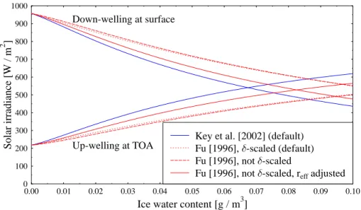
tical properties, as described in Sect.2.3.3. In this example we compare the different parameterizations and their impact on the calculated solar flux. For the example we have chosen a homogeneous ice cloud between 9 and 10 km. The ice water content (IWC) was varied between 0 and 0.1 g/cm3and the effective radius was 20 µm.

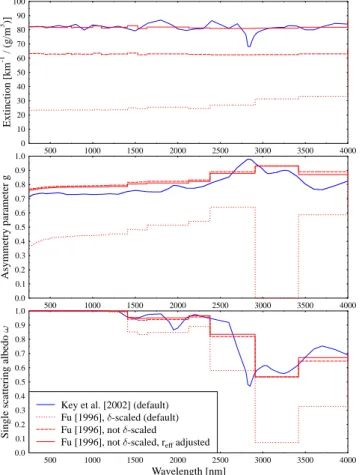
Figure 9 shows ice cloud optical properties as provided by two parameterizations

25

included in uvspec. The solid blue line is a 56-band parameterization by Key et al.

(2002) which uses a double Henyey-Greenstein approximation of the phase function that properly describes the forward and backward peak. It has been shown that this

(26)

ACPD

5, 1319–1381, 2005

The

EGU

parameterization is even suited for the calculation of radiances, e.g. Gonzalez et al.

(2002). Key et al. (2002) allows a choice of six different particle habits, and for this

example we selected solid (hexagonal) columns. The dashed red line is the parame-terization byFu(1996). The huge difference between both parameterizations is mostly explained by the fact thatFu(1996) use delta-scaled optical properties whileKey et al.

5

(2002) provide unscaled properties. Delta-scaling means a truncation of the forward peak which is added to the direct (transmitted) radiation, seeFu(1996) for details. In consequence, the phase function is much smoother and can be safely approximated by a Henyey-Greenstein phase function; and, the optical thickness, single scattering albedo, and asymmetry factor are reduced. The figure clearly shows that this

reduc-10

tion can be rather severe, e.g. a factor of about 3 for the optical thickness in the visible spectral range. While delta-scaling is important for two-stream approximations or the four-stream method by Fu and Liou (1992), its relevance is smaller when the disort solver is chosen. First, disort is able to handle the phase function in full detail; second, disort does a delta-scaling internally anyway. In consequence, the radiation calculated

15

by disort is only slightly affected by the delta-scaling, see Fig. 10: The blue line is again the parameterization byKey et al. (2002). By default, uvspec uses the delta-scaled optical properties by Fu (1996) as recommended there (dotted red line), but using an input parameteric fu tau unscaled allows to switch delta-scaling off (dashed

red line). If one defines a cloud only by its microphysical properties (ice water content,

20

effective radius), delta-scaling should certainly be switched on. If one, however, uses theFu(1996) parameterization in combination with an explicit definition of the optical thickness, asymmetry parameter, or single scattering albedo, it might be reasonable to switch delta-scaling off. This is a complicated and confusing topic and it is recom-mended that the user experiments with the options, reads the paper byFu(1996), and

25

makes heavy use of theverbose feature.

Even after switching off delta-scaling, large differences remain between theKey et al.

(2002) and Fu (1996) parameterizations (Fig. 9): The reason is the use of different definitions of the effective radius by both authors. While for spherical droplets the

(27)

ACPD

5, 1319–1381, 2005

The

EGU

effective radius is a clearly defined quantity, several different definitions of the effective radius exist for non-spherical particles (McFarquhar and Heymsfield, 1998). Careful evaluation of the formulas leads to the result that, for the same hexagonal particle, the effective radius would be 3√3/4=1.299 times larger following theKey et al.(2002) definition than theFu(1996) definition. Another option,ic fu reff yang, allows to use 5

the effective radius definition of Key et al.(2002) in the Fu (1996) parameterization. This explains most of the remaining differences, see solid red lines in Figs. 9 and

10. The remaining difference in the irradiances is mostly caused by the asymmetry parameter. Key et al.(2002) use a double Henyey-Greenstein phase function with a small backward peak. This makes the asymmetry parameter somewhat smaller than in

10

theFu(1996) parameterization, causing more reflected and less transmitted irradiance. 4.4. Inhomogeneous clouds (uvspec)

Clouds are inherently inhomogeneous at all spatial scales. To treat this inhomogene-ity properly, two things are required: First, a radiative transfer equation solver which allows to consider inhomogeneity, e.g. MYSTIC. Second, the three-dimensional

distri-15

bution of liquid water content and droplet or particle size. To demonstrate the treatment of inhomogeneous clouds in libRadtran we chose the second case of the Intercompar-ison of 3-D Radiation codes (I3RC, 1999, Cahalan et al., revised, 20042). The two-dimensional cloud field is based on extinction retrievals from the MMCR (Millimeter Cloud Radar) and the MWR (microwave radiometer) at the ARM CART site in

Okla-20

homa on 8 February 1998. The field consists of 640 columns along the x-direction, which were set to have a 50 m horizontal width (for the 10 s measurements this corre-sponds to the observed wind speed of ∼5 m/s), and each column is resolved into 54 vertical layers which are 45 meters thick (z-direction). It is assumed that the cloud is in-finite along the y-direction. In deviation from the original data set some inhomogeneity

25

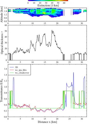
was added by cutting off the optically thin regions: Columns with an integrated optical thickness of less than 10 were declared cloudless which resulted in a cloud cover of 82%, see top and middle panels of Fig.11.

(28)

ACPD

5, 1319–1381, 2005

The

EGU

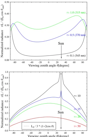
For simplicity, the asymmetry parameter was set to a constant value of 0.85 and a single scattering albedo of 1 was assumed which are reasonable assump-tions for the visible spectral range. Although it is easily included in the calcula-tion, the background molecular atmosphere was switched off using no rayleigh and

no molecular absorption. The solar zenith angle was 30◦ with the sun shining from

5

the left side. The bottom plot of Fig. 11 compares the results of three methods to calculate the transmittance at cloud bottom, z=0.6 km. The most accurate yet most time-consuming calculation is the three-dimensional Monte Carlo (MYSTIC) calcula-tion which gives to our knowlegde exact results (blue curve). Indeed, for this simple case, 13 out of 16 contributing models (including MYSTIC) agreed within ±0.5% in the

10

Intercomparison of 3-D radiation codes (I3RC,1999, Cahalan et al., revised, 20042). In comparison, the red curve shows the independent pixel approximation which involves 640 calls to DISORT2, one for each individual cloud column, usingwc ipa files.

Com-paring both results, a few typical three-dimensional features become obvious. First, the independent pixel approximation resembles the variations of the optical thickness

15

distribution much closer than the three-dimensional simulation. The much smoother variation of the radiation field in the exact calculation is caused by net horizontal photon diffusion which results in so-called “radiative smoothing” (Marshak et al.,1995). Sec-ond, in the cloud gaps, the transmittance might be considerably enhanced compared to the theoretical cloudless value Tcloudless= cos(30◦)=0.86603. Actually, the maximum

20

calculated value is 1.48 which is 70% higher than the independent-pixel maximum of 0.86603. Finally, the transmittance field is shifted away from the sun compared to the optical thickness distribution which is clearly again a result of net horizontal photon transport. Despite these effects which are not correctly reproduced by the independent-column approximation, the area averages are surprisingly close. While

25

the correct MYSTIC transmittance is 0.412, the independent pixel approximation gives 0.414 which is only 0.5% higher. It has been shown that the independent pixel approx-imation may give quite correct results for the averaged transmittance or reflection, in particular for overcast conditions (Cahalan et al.,1994a,b), although possibly for the

(29)

ACPD

5, 1319–1381, 2005

The

EGU

wrong reason as the detailed analysis above has shown. In real applications, how-ever, the detailed distribution of optical properties is often not known in which case a much simpler approximation is required. One example is shown, usingwc cloudcover 0.82344. With this option, only two independent calculations are done, for a clear

col-umn and a cloudy colcol-umn using the average extinction coefficient profile over all cloudy

5

columns. Using this fast approximation which requires only little knowledge of the ac-tual cloud structure a cloudless transmittance of 0.86603 and a cloud transmittance of 0.28599 are obtained (green curve in Fig.11). The cloudcover-weighted average returned by libRadtran is 0.388 which is 6% lower than the correct three-dimensional result. The deviation which is due to the cloudy fraction only is the so-called

plane-10

parallel bias, a systematic over-estimation of the reflection and under-estimation of the transmittance when the variability of the cloud properties is neglected (Cahalan et al.,

1994a). This example is by no means extreme, and larger as well as smaller di

ffer-ences between the three approaches may be obtained depending on cloud geometry as well as solar zenith angle.

15

4.5. Ozone, clouds, and doserates (Gen o3 tab.pl, Gen wc tab.pl, read o3 tab) Spectral information may be used to derive information about the state of the atmo-sphere. Stamnes et al.(1991) proposed methods to derive the ozone column and the cloud optical thickness from measured UV spectra. This method was subsequently adopted to multichannel moderate bandwidth filter instruments by Dahlback (1996).

20

Tools for generation of the necessary lookup tables are included within libRadtran. Gen o3 tab.pl generates lookup tables for the retrieval of the ozone column from down-welling irradiance or zenith radiance ratios. The ratios are made of radiation from one wavelength or wavelength interval that is sensitive to ozone absorption and one that has low sensitivity. The lookup table of the total ozone column is a function of the solar

25

zenith angle and the ratio. Similarily Gen wc tab.pl generates lookup tables for estima-tion of effective cloud optical thickness and/or sky transmittance from global irradiance measurements at a single wavelength or wavelength interval. By effective cloud optical

(30)

ACPD

5, 1319–1381, 2005

The

EGU

thickness is meant the optical thickness that, when used as input to the model, best reproduces the measurements. Hence, the effective cloud optical thickness includes both aerosol and cloud contributions. The lookup tables are read by the read o3 tab program that returns the total ozone column or cloud information depending on the lookup table and additional input information.

5

Examples of the use of these tools are provided in Fig.12.

The CIE doserate (McKinlay and Diffey,1987) as derived from a Ground-based Ul-traviolet Radiometer (GUV-541, Biospherical Instruments Inc., San Diego, USA) multi-channel moderate bandwidth filter instrument is shown in black. The CIE dose at noon is the basis for deriving the UV-index (International Commision on Non-Ionizing

Radia-10

tion Protection,1995). Data are from Julian day 172 (21 June 1997), Tromsø, Norway and are shown at one minute resolution. Both the measurements and the methods become less reliable at large solar zenith angle, thus results shown are for solar zenith angles ≤80◦.

Between 04:00 and 09:00 the sky was cloudless. This is reflected both in the CIE

15

doserate and the cloud optical thickness, the latter being zero for this time interval. Around noon some clouds start to appear. The clouds are broken and occasionally cause CIE doserates higher than the corresponding cloudless values. In the afternoon the clouds get slightly denser with optical thickness between 1.5 and 11.

The ozone column average over the day is (369±13) DU. Some variations are seen

20

in the derived column. Some are due to uncertainties associated with the method and the measurements. For example for large solar zenith angles the lookup table is sensitive to the ozone profile. Also some cloud influence is evident.Mayer et al.(1998) described that enhanced absorption of UV radiation may take place due to multiple scattering in clouds. This may lead to unrealistically large ozone columns with this

25

method for ozone retrieval. Thus, it is customary to ignore ozone values for large cloud optical thickness.

Some of these methods have been used by for example Leontyeva and Stamnes