HAL Id: cea-01234364
https://hal-cea.archives-ouvertes.fr/cea-01234364
Submitted on 26 Nov 2015
HAL is a multi-disciplinary open access
archive for the deposit and dissemination of
sci-entific research documents, whether they are
pub-lished or not. The documents may come from
teaching and research institutions in France or
abroad, or from public or private research centers.
L’archive ouverte pluridisciplinaire HAL, est
destinée au dépôt et à la diffusion de documents
scientifiques de niveau recherche, publiés ou non,
émanant des établissements d’enseignement et de
recherche français ou étrangers, des laboratoires
publics ou privés.
Gas-to-dust mass ratios in local galaxies over a 2 dex
metallicity range
Aurélie Rémy-Ruyer, S. C. Madden, F. Galliano, M. Galametz, T. T.
Takeuchi, R. S. Asano, S. Zhukovska, V. Lebouteiller, D. Cormier, A. Jones,
et al.
To cite this version:
Aurélie Rémy-Ruyer, S. C. Madden, F. Galliano, M. Galametz, T. T. Takeuchi, et al.. Gas-to-dust
mass ratios in local galaxies over a 2 dex metallicity range. Astronomy and Astrophysics - A&A, EDP
Sciences, 2014, 563, pp.A31. �10.1051/0004-6361/201322803�. �cea-01234364�
DOI:10.1051/0004-6361/201322803
c
ESO 2014
Astrophysics
&
Gas-to-dust mass ratios in local galaxies
over a 2 dex metallicity range
?
A. Rémy-Ruyer
1, S. C. Madden
1, F. Galliano
1, M. Galametz
2, T. T. Takeuchi
3, R. S. Asano
3, S. Zhukovska
4,5,
V. Lebouteiller
1, D. Cormier
5, A. Jones
6, M. Bocchio
6, M. Baes
7, G. J. Bendo
8, M. Boquien
9, A. Boselli
9,
I. DeLooze
7, V. Doublier-Pritchard
10, T. Hughes
7, O. Ł. Karczewski
11, and L. Spinoglio
121 Laboratoire AIM, CEA/IRFU/Service d’Astrophysique, Université Paris Diderot, Bat. 709, 91191 Gif-sur-Yvette, France
e-mail: [email protected]
2 Institute of Astronomy, University of Cambridge, Madingley Road, Cambridge CB3 0HA, UK
3 Division of Particle and Astrophysical Science, Nagoya University, Furo-cho, Chikusa-ku, Nagoya 464-8602, Japan 4 Max-Planck-Institut für Astronomie, Königstuhl 17, 69117 Heidelberg, Germany
5 Zentrum für Astronomie der Universität Heidelberg, Institut für Theoretische Astrophysik, Albert-Ueberle-Str. 2,
69120 Heidelberg, Germany
6 Institut d’Astrophysique Spatiale, CNRS, UMR8617, 91405 Orsay, France
7 Sterrenkundig Observatorium, Universiteit Gent, Krijgslaan 281 S9, 9000 Gent, Belgium
8 UK ALMA Regional Centre Node, Jodrell Bank Centre for Astrophysics, School of Physics & Astronomy,
University of Manchester, Oxford Road, Manchester M13 9PL, UK
9 Laboratoire d’Astrophysique de Marseille – LAM, Université d’Aix-Marseille & CNRS, UMR7326, 38 rue F. Joliot-Curie,
13388 Marseille Cedex 13, France
10 Max Planck für Extraterrestrische Physik, Giessenbachstr. 1, 85748 Garching, Germany 11 Department of Physics and Astronomy, University of Sussex, Brighton, BN1 9QH, UK
12 Instituto di Astrofisica e Planetologia Spaziali, INAF-IAPS, via Fosso del Cavaliere 100, 00133 Roma, Italy
Received 5 October 2013/ Accepted 9 December 2013
ABSTRACT
Aims.The goal of this paper is to analyse the behaviour of the gas-to-dust mass ratio (G/D) of local Universe galaxies over a wide
metallicity range. We especially focus on the low-metallicity part of the G/D vs metallicity relation and investigate several explanations for the observed relation and scatter.
Methods.We assembled a total of 126 galaxies, covering a 2 dex metallicity range and with 30% of the sample with 12+ log(O/H) ≤
8.0. We homogeneously determined the dust masses with a semi-empirical dust model including submm constraints. The atomic and molecular gas masses have been compiled from the literature. We used two XCO scenarios to estimate the molecular gas mass: the
Galactic conversion factor, XCO,MW, and a XCOthat depends on the metallicity XCO,Z(∝Z−2). We modelled the observed trend of the
G/D with metallicity using two simple power laws (slope of –1 and free) and a broken power law. Correlations with morphological type, stellar masses, star formation rates, and specific star formation rates are also discussed. We then compared the observed evolution of the G/D with predictions from several chemical evolution models and explored different physical explanations for the observed scatter in the G/D values.
Results.We find that out of the five tested galactic parameters, metallicity is the main physical property of the galaxy driving the
observed G/D. The G/D versus metallicity relation cannot be represented by a single power law with a slope of –1 over the whole metallicity range. The observed trend is steeper for metallicities lower than ∼8.0. A large scatter is observed in the G/D values for a given metallicity: in metallicity bins of ∼0.1 dex, the dispersion around the mean value is ∼0.37 dex. On average, the broken power law reproduces the observed G/D best compared to the two power laws (slope of –1 or free) and provides estimates of the G/D that are accurate to a factor of 1.6. The good agreement of observed values of the G/D and its scatter with respect to metallicity with the predicted values of the three tested chemical evolution models allows us to infer that the scatter in the relation is intrinsic to galactic properties, reflecting the different star formation histories, dust destruction efficiencies, dust grain size distributions, and chemical compositions across the sample.
Conclusions.Our results show that the chemical evolution of low-metallicity galaxies, traced by their G/D, strongly depends on their
local internal conditions and individual histories. The large scatter in the observed G/D at a given metallicity reflects the impact of various processes occurring during the evolution of a galaxy. Despite the numerous degeneracies affecting them, disentangling these various processes is now the next step.
Key words.evolution – galaxies: dwarf – galaxies: evolution – galaxies: ISM – infrared: ISM – dust, extinction
1. Introduction
Metallicity is a key parameter in studying the evolution of galax-ies because it traces metal enrichment. Elements are injected by
?
Appendices are available in electronic form at http://www.aanda.org
stars in the interstellar medium (ISM) via stellar winds and/or supernovae (SN) explosions (Dwek & Scalo 1980) and become available for the next generation of stars. The metallicity a pri-ori traces the history of the stellar activity of a galaxy, i.e., the number of stellar generations already produced. Metallicity is thus expected to increase with age as the galaxy undergoes
chemical enrichment through successive star formation events. However, this metal enrichment is in fact a more complex pro-cess and depends on external and internal propro-cesses occurring during galaxy evolution. Indeed, the gas phase abundance can be affected by metal-poor gas inflows that will dilute the ISM
(Montuori et al. 2010;Di Matteo et al. 2011) and decrease the
metallicity of the galaxy or by outflows driven by stellar feed-back (stellar winds or SN shocks; e.g.,Dahlem et al. 1998;Frye
et al. 2002) that will eject metal-rich gas into the intergalactic
medium, again resulting in a galaxy whose metallicity does not simply increase with time. Elements are also processed by gas and dust in the ISM. Dust grains form from the available met-als in the ISM, and those metmet-als can thus be depleted from the gas phase (Savage & Sembach 1996;Whittet 2003). Metals are returned to the gas phase when dust is destroyed (e.g., by SN blast waves,Jones et al. 1994,1996). The gas-to-dust mass ra-tio (G/D) links the amount of metals locked up in dust with that still present in the gas phase and is thus a powerful tracer of the evolutionary stage of a galaxy. Investigations of the rela-tion between the observed G/D and metallicity can thus place strong constraints on the physical processes governing galaxy evolution and, more specifically, on chemical evolution models. Because of their low metallicity, dwarf galaxies can be consid-ered as chemically young objects that are at an early stage in their evolution. In this picture, they can be seen as our closest analogues of the primordial environments present in the early Universe, from which the present-day galaxies formed. G/D of dwarf galaxies are thus crucial for constraining chemical evolu-tion models at low metallicities.
The observed G/D of integrated galaxies as a function of metallicity has been intensively studied over the past decades (e.g.,Issa et al. 1990;Lisenfeld & Ferrara 1998;Hirashita et al.
2002; James et al. 2002; Hunt et al. 2005;Draine et al. 2007;
Engelbracht et al. 2008; Galliano et al. 2008; Muñoz-Mateos
et al. 2009;Bendo et al. 2010;Galametz et al. 2011; Magrini
et al. 2011). In the disk of our Galaxy, the proportion of heavy
elements in the gas and in the dust has been shown to scale with the metallicity (Dwek 1998) if one assumes that the time de-pendence of the dust formation timescale is the same as that of the dust destruction timescale. This results in a constant dust-to-metal mass ratio and gives a dependence of the G/D on metallic-ity as G/D ∝ Z−1(that we call hereafter the “reference” trend).
This reference trend between G/D and metallicity seems con-sistent with the observations of galaxies with near-solar metal-licities (e.g.,James et al. 2002;Draine et al. 2007;Bendo et al.
2010;Magrini et al. 2011). However, some studies also show that
the G/D of some low-metallicity dwarf galaxies deviate from this reference trend, with a higher G/D than expected for their metal-licity (Lisenfeld & Ferrara 1998; Galliano et al. 2003, 2005,
2008,2011;Hunt et al. 2005;Bernard et al. 2008;Engelbracht
et al. 2008;Galametz et al. 2011).
The G/D is often used to empirically estimate the “CO-free” molecular gas. This molecular gas, not directly traced by CO measurements, was first proposed in low-metallicity galaxies us-ing the 158 µm [C] line (Poglitsch et al. 1995;Israel et al. 1996;
Madden et al. 1997,2012). Alternatively, using the dust mass
determined from far-infrared (FIR) measurements and assuming a G/D, given the metallicity of the galaxy, a gas mass can be estimated. This gas mass is then compared to the observed H and CO gas masses to estimate the “CO-free” gas mass. This method is also used to estimate the CO-to-H2 conversion factor in local (e.g.,Guelin et al. 1993,1995; Neininger et al. 1996;
Boselli et al. 2002;Sandstrom et al. 2013) and high-z galaxies
(e.g.,Magdis et al. 2012;Magnelli et al. 2012). However, using
these methods requires an accurate estimation of the G/D at a given metallicity.
A certain number of instrumental limitations and/or model caveats have limited former studies of the G/D. First, limits in wavelength coverage in the FIR have hampered precise de-termination of the dust masses. For the earliest studies, the dust masses were derived from IRAS or Spitzer measurements, not extending further than 100–160 µm, therefore not tracing the cooler dust. As the bulk of the dust mass in galaxies of-ten resides in the cold dust component, this has strong conse-quences for the dust mass and the G/D determination. Before Herschel, using Spitzer and ground-based data,Galametz et al.
(2011) indeed showed that a broad wavelength coverage of the FIR-to-submillimetre (submm) part of the spectral energy dis-tribution (SED) was critical to obtain accurate estimates of the dust masses. Second, some of the studies presented previously used modified blackbody models to derive dust masses. Using Herschel data and a semi-empirical dust model, Dale et al.
(2012) showed that the dust mass modelled with a modified blackbody could be underestimated by a factor of ∼2.Bianchi
(2013) showed, on the contrary, that a modified blackbody mod-elling, using a fixed emissivity index, provides a good estimate of the dust mass. However, the case of low-metallicity dwarf galaxies has not been investigated yet and the two dust mass estimates may not be consistent with each other at low metallici-ties. And finally, the limited sensitivities of the pre-Herschel era instruments only allowed the detection of dust for the brightest and highest-metallicity dwarf galaxies, limiting G/D studies to metallicities ≥1/5 Z 1(12+ log(O/H) = 8.0).
In this work we investigate the relation between the G/D and metallicity avoiding the limitations and caveats mentioned in the previous paragraph. Using new Herschel data to constrain a semi-empirical dust model, we have a more accurate determi-nation of the dust masses comparing to Spitzer-only dust masses and/or modified blackbody dust masses. Our sample also cov-ers a wide range in metallicity (2 dex, from 12+ log(O/H) = 7.1 to 9.1), with a significant fraction of the sample below 12+ log(O/H) = 8.0 (∼30%, see Sect.2), thanks to the increased sensitivity of Herschel which enables us to access the dust in the lowest metallicity galaxies. We are thus able to provide better constraints on the G/D at low metallicities.
In Sect.2, we describe the sample and the method used to estimate the dust and total gas masses. Then we investigate the relation of the observed G/D with metallicity and other galac-tic parameters in Sect.3 and fit several empirical relations to the data. We then interpret our results with the aid of several chemical evolution models in Sect.4. Throughout we consider (G/D) = 1622(Zubko et al. 2004).
2. Sample and masses
2.1. Sample
We combine 3 different samples for our study of the G/D: the Dwarf Galaxy Survey (DGS, Madden et al. 2013), the KINGFISH survey (Kennicutt et al. 2011) and a subsample of the sample presented inGalametz et al.(2011, called the “G11 sample” hereafter). The basic parameters for all of the galaxies 1 Throughout we assume (O/H)
= 4.90 × 10⁻⁴, i.e., 12 +
log(O/H) = 8.69, and a total solar mass fraction of metals Z = 0.014
(Asplund et al. 2009).
2 This value is from Table 6 fromZubko et al.(2004) for the
BARE-GR-S model, which corresponds to the dust composition used for our modelling (see Sect.2.2).
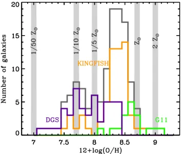
Fig. 1. Metallicity distribution of the DGS (purple), KINGFISH (or-ange) and G11 (green) samples from 12+ log(O/H) = 7.14 to 9.10. The total distribution is indicated in grey. Solar metallicity is indicated here as a guide to the eye, as well as the 1/50, 1/10, 1/5 and 2 Z values.
such as positions and distances can be found inMadden et al.
(2013) for the DGS;Kennicutt et al.(2011) for KINGFISH; and
Galametz et al.(2011) for the G11 sample.
The DGS sample consists of 48 star-forming dwarf galaxies (mostly dwarf irregulars and blue compact dwarfs (BCDs)) cov-ering metallicities from 12+ log(O/H) = 7.14 to 8.43, whereas the KINGFISH sample probes more metal-rich environments (61 galaxies including spiral, early-type and a few irregular galaxies), from 12+ log(O/H) = 7.54 to 8.77. The G11 sam-ple consists of all of the galaxies inGalametz et al.(2011) that are neither already in the DGS nor in the KINGFISH samples, and except those galaxies which show a submm excess (see Sect.2.2). This gives 17 additional galaxies, mostly solar or su-per solar environments (mostly spiral galaxies), with metallici-ties from 12+ log(O/H) = 8.14 to 9.10. The metallicity distribu-tion for each of the 3 samples is presented in Fig.1.
All of these metallicities have been derived using empiri-cal strong emission line methods (see Madden et al. 2013, for the DGS, Kennicutt et al. 2011 for KINGFISH and Galametz et al. 2011 for G11 metallicity determination). The DGS and KINGFISH metallicities have been obtained through the R23
ra-tio3 with the Pilyugin & Thuan (2005) calibration. Galametz
et al.(2011) do not indicate precisely which calibration they use
to convert R23 into metallicity, thus several metallicities for the
G11 galaxies were re-estimated from the original line intensities, available in the literature, with thePilyugin & Thuan(2005) cal-ibration. We also assume a conservative 0.1 dex uncertainty for the G11 metallicities. On average for the total sample, the uncer-tainty on the metallicity measurements is ∼0.1 dex. The metallic-ities for the whole sample are listed in TableA.1. Other methods exist to determine metallicities and can lead to very different val-ues, but this will only introduce a systematic offset in the adopted values here (Kewley & Ellison 2008). Note that these metallicity values correspond to global estimates. On smaller scales within galaxies, differences can occur due to inhomogeneous mixing of metals: metallicity gradients have been observed in large spiral 3 R
23= ([OII]λ3727+[OIII]λλ4959, 5007)/Hβ.
galaxies (Garnett et al. 2004;Bendo et al. 2010;Moustakas et al. 2010). Dwarf galaxies, however, are smaller in size than metal-rich galaxies and we can presume, for this study, that metallic-ity is more homogeneous within these environments (Revaz &
Jablonka 2012;Valcke et al. 2008).
This gives us a total of 126 galaxies spanning a 2 dex range in metallicity (Fig.1). We see that the low-metallicity end of the distribution is fairly well sampled as we have ∼30% of the total sample with metallicities below 1/5 Z .
2.2. Dust masses
To ensure a consistent determination of the dust masses through-out our sample, all of the galaxies are modelled with the dust SED model presented in Galliano et al. (2011). It is a phe-nomenological model based on a two steps approach: first the modelling of one mass element of the ISM with a uniform il-lumination, and second the synthesis of several mass elements to account for the different illumination conditions. In the first step we assume that the interstellar radiation field (ISRF) has the spectral shape of the solar neighbourhood ISRF (Mathis et al. 1983) and use theZubko et al.(2004) grain properties with up-dated PAH optical properties fromDraine & Li(2007). In the second step, we assume that the total SEDs of the galaxies can be well represented by the combination of the emission from regions with different properties. In order to do so, we assume that the dust properties are uniform and that only the illumina-tion condiillumina-tions vary in the different regions. The various regions are then combined using theDale et al.(2001a) prescription: the distribution of the starlight intensities per unit dust mass can be represented by a power law:
dMdust
dU ∝ U
−αU with U
min≤ U ≤ Umin+ ∆U (1)
where Mdustis the dust mass, U is the starlight intensity and αU
is the index of the power law describing the starlight intensity distribution.
We use the “standard” grain composition in our model, i.e., PAHs, silicate dust and carbon dust in form of graphite4. The
submm emissivity index, β, for this grain composition is ∼2.0
(Galliano et al. 2011). We discuss the impact of having another
dust composition on our results (e.g., the use amorphous carbons instead of graphite grains) in Sect.3.4.
The free parameters of the model are: the dust mass, Mdust,
the minimum starlight intensity, Umin, the difference between the
maximum and minimum starlight intensities,∆U, the starlight intensity distribution power-law index, αU, the PAH-to-total dust
mass ratio, fPAH, the mass fraction of ionised PAHs compared to
the total PAH mass, fion, the mass fraction of very small grains
(i.e., non-PAH grains with sizes ≤10 nm), fvsg, and the
contri-bution of the near-IR stellar continuum, Mstar(seeGalliano et al.
2011, for details and a full description of the model). This model has previously been used to model dwarf galaxies, notably by
Galametz et al.(2009,2011);O’Halloran et al.(2010);Cormier
et al.(2010);Hony et al.(2010);Meixner et al.(2010).
For the DGS sample, we collect IR-to-submm photometri-cal data from various instruments (i.e., 2MASS, Spitzer, WISE, IRAS, and Herschel) for the largest possible number of galax-ies. IRS spectra are also used to constrain the MIR slope of the SEDs. For 12 DGS galaxies, the MIR continuum shape outlined by the IRS spectrum cannot be well fitted by our model. In these cases, we add an extra modified blackbody component in the 4 This corresponds to the BARE-GR-S model ofZubko et al.(2004).
MIR, with a fixed β = 2.0 and a temperature varying between 80 and 300 K. This affect our dust masses by ∼5%, which is well within the error bars for the dust masses (∼26%), and thus this does not affect our following results. For one DGS galaxy, SBS1533+574, the impact on the dust mass is significant, but the addition of this warm modified blackbody is necessary to have a MIR-to-submm shape of the SED consistent with the observations (Rémy-Ruyer et al., in prep.) Out of the 48 DGS galaxies, only five do not have enough constraints (i.e., no ob-servations are available or there are too many non-detections) to obtain a dust mass. Herschel data for the DGS is presented in
Rémy-Ruyer et al.(2013). 2MASS, WISE and IRAS flux
den-sities for the DGS are compiled from the NASA/IPAC IRSA databases and the literature. Spitzer-MIPS measurements are taken fromBendo et al.(2012). Spitzer-IRAC and IRS data to-gether with a complete description of the dust modelling and the presentation of the final SEDs and dust masses for the DGS galaxies are presented in Rémy-Ruyer et al. (in prep.).
For the KINGFISH sample, we use IR-to-submm fluxes from
Dale et al.(2007,2012) to build the observed SEDs (i.e.,
obser-vational constraints from 2MASS, Spitzer, IRAS and Herschel).
TheDale et al.(2012) fluxes have been updated to the new values
of the SPIRE beam areas5. The dust masses for the KINGFISH
galaxies are presented in Table A.2. A submm excess is ob-served in some DGS and KINGFISH galaxies at 500 µm (Dale
et al. 2012; Rémy-Ruyer et al., in prep.). If present, the excess
is rather small at 500 µm and can increase as we go to longer wavelengths. However, because of the unknown origin of this excess and because of the uncertainties it can bring in the dust mass estimation, we do not attempt to model this excess with ad-ditional modifications to the model, and we thus leave aside the 500 µm point in our model. Including the 500 µm point results in a median difference of ∼3% for the dust masses in the DGS and KINGFISH samples. We discuss the influence of the presence of a submm excess in Sect.3.4.
We also model galaxies from the G11 sample, as some model assumptions were different in Galametz et al. (2011). Herschelconstraints are not present but other submm constraints are taken into account such as JCMT/SCUBA at 850 µm and/or APEX/LABOCA at 870 µm, allowing a precise determination of the dust masses (given in TableA.2).Galametz et al.(2011) also observed a submm excess in nine galaxies of their original sample and modelled it with a very cold dust (VCD) compo-nent. However, the submm excess is not fully understood yet and this extra VCD component may lead to an overestimation of the dust mass. Because we do not have constraints between 160 µm and the available ground-based submm fluxes to see where the submm excess starts, we do not consider nor model these galax-ies here.
The wavelength coverage is not exactly the same from galaxy to galaxy. The most important constraints for the deter-mination of the dust mass are constraints sampling the peak of the dust SED. Herschel provides such constraints for all of the DGS and KINGFISH galaxies. Some dwarf galaxies are not de-tected with Herschel at submm wavelengths (from or beyond 160 µm) and are noted in Fig.4(see Sect.2.3). These galaxies harbour particularly warm dust (Rémy-Ruyer et al. 2013); the peak of their SED is thus shifted towards shorter wavelengths and is then well sampled by constraints until 160 µm where 5 SPIRE photometer reference spectrum values:
http://herschel.esac.esa.int/twiki/bin/view/Public/ SpirePhotometerBeamProfileAnalysis: 465, 822 and 1768 square arcseconds at 250, 350, 500 µm (September 2012 values).
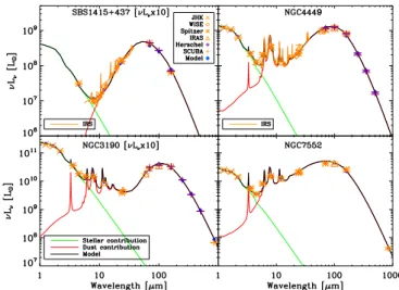
Fig. 2. Examples of SEDs modelled with the Galliano et al.(2011) model: (top left) SBS1415+437, (top right) NGC 4449, (bottom left) NGC 3190 and (bottom right) NGC 7552. The SEDs have been multi-plied by 10 for SBS1415+437 and NGC 3190 for display purposes. The observed SED includes the Herschel data (purple crosses) as well as an-cillary data (in orange). The different symbols code for the different in-struments: Xs for 2MASS bands, diamonds for WISE, stars for Spitzer IRAC and MIPS, triangles for IRAS and orange crosses for SCUBA. The IRS spectrum is also displayed in orange for the two DGS galax-ies. The total modelled SED in black is the sum of the stellar (green) and dust (red) contributions. The modelled points in the different bands are the filled blue circles.
the galaxy is still detected. For galaxies in the G11 sample, the peak of the dust SED is probed by Spitzer and/or IRAS ob-servations and the Rayleigh-Jeans slope of the SED by longer submm wavelength observations. Thus we are confident in the dust masses we derive with these sets of constraints. As an il-lustration, four SEDs are presented in Fig. 2: one very low-metallicity DGS galaxy (SBS1415+437, 12 + log(O/H) = 7.55) not observed with SPIRE, one low-metallicity DGS galaxy (NGC 4449, 12+ log(O/H) = 8.20), and two spiral galaxies from the KINGFISH sample (NGC 3190, 12+ log(O/H) = 8.49) and from the G11 sample (NGC 7552, 12+ log(O/H) = 8.35).
The errors on the dust masses are estimated by generating 300 random realisations of the SED, perturbed according to the random and systematic noise, in order to get a distribution for the dust mass. The error bars on the dust mass are taken to be the 66.67% confidence interval of the distribution (i.e., the range of the parameter values between 0.1667 and 0.8333 of the repar-tition function). The detailed procedure of the error estimation is presented in Rémy-Ruyer et al. (in prep.).
2.3. Gas masses
H masses – The H masses and their errors are compiled from the literature, and rescaled to the distances used here. Most of the atomic gas masses are given inGalametz et al.(2011) for the G11 sample, and inDraine & Li(2007) for the KINGFISH survey. They are presented inMadden et al.(2013) for the DGS. The errors were not available for all of the H measurements. When no error was available for the H mass, we adopted the mean value of all of the relative errors on the H masses compiled from the literature: ∼16%.
However, the H extent of a galaxy is not necessarily the same as the aperture used to probe the dust SED, as the H of-ten exof-tends beyond the optical radius of a galaxy (Hunter 1997).
This can be particularly true for dwarf galaxies where the H halo can be very extended: some irregular galaxies present unusu-ally extended H gas (up to seven times the optical radius,
Huchtmeier 1979;Huchtmeier et al. 1981;Carignan & Beaulieu
1989; Carignan et al. 1990; Thuan et al. 2004). We also note
that in some galaxies (e.g., NGC 4449), gas morphology may be highly perturbed due to past interactions or mergers (e.g.,Hunter
et al. 1999). This may also lead to significant uncertainties in the
H mass and thus on the derived G/D (e.g., Karczewski et al. 2013). Thus we check the literature for the DGS sample for the size of the H halo to compare it to the dust aperture. It was not possible to find this information for ∼38% of the sample (H not detected or no map available). For the rest, 25% of the DGS galaxies have a H extent that corresponds to the dust IR aper-ture, which has been chosen to be 1.5 times the optical radius (for most cases, seeRémy-Ruyer et al. 2013); and 35% have a H halo that is more extended. If we assume that the H mass distribution follows a Gaussian profile (based on the observed high central gas concentration seen in BCDs, e.g.,van Zee et al.
1998,2001;Simpson & Gottesman 2000), we can correct the
to-tal H mass for these galaxies to find the H mass corresponding to the dust aperture. In reality, the H profile can show a com-plicated structure with clumps and shells, rendering the profile more assymetric.
Our correction corresponds to a factor of ∼1.55 on aver-age, for these galaxies. Several studies (Thuan & Martin 1981;
Swaters et al. 2002;Lee et al. 2002;Begum & Chengalur 2005;
Pustilnik & Martin 2007) have tried to quantify the extent of the
H halo for dwarf galaxies and found that the ratio of H size to the optical size is typically 2, which gives a correction of ∼1.4. The atomic gas masses for the sample, after correction if needed, are presented in TableA.1.
H2masses – The H2masses have been compiled from the
liter-ature. They have been rescaled, when necessary, to the distance adopted here to derive the dust masses.
The molecular gas mass is usually derived through CO mea-surements as H2 is not directly observable. There are two main
issues in determining the molecular gas masses. First, detection of CO in low-metallicity galaxies is challenging: sensitivity has limited CO detections to galaxies with 12+ log(O/H) & 8.0 (e.g.,
Leroy et al. 2009;Schruba et al. 2012). The other issue in the H2
mass determination is the choice of the conversion factor be-tween CO intensities and molecular gas masses, XCO. Indeed
the variation of this factor with metallicity is poorly constrained, and a number of studies have been dedicated to quantifying the dependence of XCO on metallicity (Wilson 1995; Israel 1997;
Boselli et al. 2002;Israel et al. 2003;Strong et al. 2004;Leroy
et al. 2011; Schruba et al. 2012; Bolatto et al. 2013). From a
sample of 16 dwarf galaxies, and assuming a constant H2
deple-tion timescale, Schruba et al.(2012) found a XCOscaling with
(O/H)−2. This relation takes into account possible “CO-free” gas
as the XCO conversion factor is estimated from the total
reser-voir of molecular gas needed for star formation (Schruba et al. 2012). FollowingCormier et al.(2014), we estimate the molec-ular gas masses from a constant XCOfactor using the Galactic
value: XCO,MW= 2.0 × 1020cm−2(K km s−1)−1(Ackermann et al.
2011), giving us MH2,MW, and from a XCOfactor depending on
(O/H)−2: X
CO,Z, giving us MH2,Z. This provides a conservative
range of molecular gas mass estimates that reflects how uncer-tain the molecular gas mass determination is. For this reason, we do not give any error bars on our molecular gas masses.
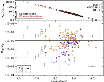
Fig. 3.Bottom: MH2/MHIas a function of metallicity for the whole
sam-ple. The blue crosses are for molecular gas masses computed with XCO,MW and the orange diamonds are for molecular gas masses
com-puted with XCO,Z. Upper limits in the molecular gas mass are
indi-cated with grey arrows and smaller grey symbols. The mean error for the data points is shown in grey on the bottom right of the plot. The plain line shows the unity line. The dashed blue and orange lines show the 1.2% and 68% molecular-to-atomic gas mass fractions respectively and represent the mean H2-to-H ratio of the detected galaxies with
12+ log(O/H) < 8.1 (see text). The horizontal dashed black line shows the metallicity threshold 12+ log(O/H) = 8.1 to guide the eye. Top: XCO,Z/XCO,MWillustrating the (O/H)−2dependence adopted to compute
XCO,Z. The symbols delineate between the three samples: crosses,
down-ward triangles and stars for the DGS, KINGFISH and G11 samples re-spectively. The colours differentiate between H2 detections (in black,
corresponding to the coloured points on the bottom panel) and the H2
non-detections (in red, corresponding to the grey points in the bottom panel).
In order to go beyond the CO upper limits and to constrain the G/D behaviour at low metallicities we find a way to estimate the amount of molecular gas for the lowest metallicity galaxies. Figure3shows the ratio of MH2-to-MHIas a function of
metallic-ity for our sample and for both cases of XCO. We note that around
12+ log(O/H) ∼ 8.1 the ratio MH2/MHI drops suddenly for the
detected galaxies for both XCO. For these very low-metallicity
galaxies with 12+ log(O/H) ≤ 8.1, the mean ratio between the detected MH2and MHIis 1.2%, for XCO,MW. Using XCO,Z, this
ra-tio goes up to 68%. Thus for galaxies with non-detecra-tions in CO or without any CO observations, and with 12+ log(O/H) ≤ 8.1, we replace the upper limit values by 0.012 × MHIfor MH2,MWand
0.68 × MHIfor MH2,Z. Given the low molecular gas fraction we
find, this will not greatly affect our interpretation of G/D nor the conclusions. From now on, the galaxies for which we apply this correction will be treated as detections. This 12+ log(O/H) value of ∼8.1 has already been noted as being special for dwarf galax-ies (e.g., for the strength of the PAH features:Engelbracht et al.
2005,2008;Madden et al. 2006;Draine et al. 2007;Galliano
et al. 2008). The molecular gas masses we use in the following
analysis are presented in TableA.1.
Total gas masses – We get the total gas mass, Mgas, by adding
all of the different gas contributions: the atomic gas mass, the molecular gas mass, the helium gas mass and the gaseous metal mass:
a)
b)
c)
d)
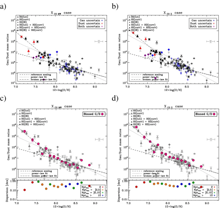
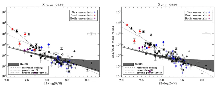
Fig. 4.Top row: G/D as a function of metallicity for the 2 values of XCO: XCO,MWa) and XCO,Zb). The mean error for the data points is shown in
grey on the right of the plots. The colours code the reliability of the point depending whether the gas mass is uncertain (in blue), the dust mass is uncertain (in red) or if both are uncertain (in purple). The symbol traces the changes made in the H and H2masses (see text for details on the
uncertainties and the changes on the gas masses). The dashed line represents the reference scaling of the G/D with metallicity (not fit to the data). The dotted and dash-dotted lines represent the best power-law and best broken power-law fits to the data. Bottom row: same as top row for XCO,MW
c) and XCO,Zd), where the binned G/D values (see text) have been added as pink filled circles. For clarity, the observed G/D values are now shown
in grey. On the bottom panels the relative dispersion in each bins, in terms of standard deviation, is shown and the colours show the number of galaxies in each bin.
where MHeis the helium mass and Zgalthe mass fraction of
met-als in the galaxy. Assuming MHe = Y Mgas, where Y is the
Galactic mass fraction of Helium, Y = 0.270 (Asplund et al.
2009), we have:
Mgas= µgal(MHI+ MH2), (3)
with µgal= 1/(1−Y −Zgal) the mean atomic weight. µgalhas been
computed for each galaxy and the mean value for our sample is 1.38 ± 0.01 (see TableA.1). We get Zgalassuming (Zgal/Z )=
(O/Hgal)/(O/H ) and Z = 0.014 (Asplund et al. 2009).
We assume here that the ionised gas mass (MHII) is
negligi-ble compared to the H mass. We perform the test for 67 galax-ies of the sample, with MHIIderived from Hα measurements of
Gil de Paz et al. (2003);Kennicutt et al. (2009);Skibba et al.
(2011) and found MHII/MHI∼ 0.2%. However, we found two
dwarf galaxies for which the ionised gas mass should be taken into account as it contributes equally or more than the atomic gas mass: Haro11 (MHII∼ 1.2 × MHI,Cormier et al. 2012) and
Pox186 (MHII∼ MHI,Gil de Paz et al. 2003). For these two
galax-ies, the total gas mass also includes MHII.
The G/D as a function of metallicity is presented in Figs.4a, b for the two cases: XCO,MW or XCO,Z. The average
er-ror on the observed G/D is ∼27% in both XCOcases (∼10% for
the total gas mass and ∼26% for the dust mass). The dashed line indicates the reference scaling of the G/D with metallicity. The colours of the symbols indicate the reliability of the data points by tracing if the gas or dust masses determinations are uncertain. Blue symbols refer to H or H2 non-detections or to
the absence of H2observations for the galaxy. Red symbols
The combination of both indications for the gas and dust masses is shown with the purple symbols. Black symbols indicate that both gas and dust masses have reliable measurements (67% of the sample).
The type of symbols indicates whether or not the H and/or H2masses have been corrected. For the H masses we distinguish
three cases for the DGS galaxies: the H extent of the galaxy is unknown and we cannot correct the H mass (diamonds), the H extent is known and greater than the dust aperture and we cor-rect the H mass (triangles) and the H extent is known and sim-ilar to the dust aperture, there is no need to correct the H mass (crosses). The galaxies with 12+ log(O/H) < 8.1 for which the H2 masses have been corrected (either from upper limit or lack
of measurements) are indicated as filled symbols (see paragraph above on H2masses).
3. Analysis
3.1. Observed gas-to-dust mass ratio – metallicity relation and dispersion
To evaluate the general behaviour and scatter in the G/D values at different metallicities, we consider the error-weighted mean val-ues of log(G/D) in metallicity bins (neglecting the upper/lower limits), with the bin sizes chosen to include at least two galaxies and to span at least 0.1 dex. The result is overlaid as pink filled circles in Figs.4c, d. We also look at the dispersion of the G/D values in each metallicity bin (see bottom panels of Figs.4c, d), by computing the standard deviation of the log(G/D) values in each bin (also neglecting the upper/lower limits). The dispersion is ∼0.37 dex (i.e., a factor of 2.3) on average for all bins and for both XCOvalues. Additionally, in one bin the G/D vary on
aver-age by one order of magnitude. This confirms that the relation between G/D and metallicity is not trivial even at a given metal-licity, and over the whole metallicity range. We also see that the dispersion in the observed G/D values does not depend on metal-licity. This indicates that the scatter within each bin may be in-trinsic and does not reflect systematic observational or correction errors. This also means that the metallicity is not the only driver for the observed scatter in the G/D values: other processes oper-ating in galaxies can lead to large variation in the G/D in a given metallicity range, throughout this range. However, there might be a selection bias in our sample. Indeed our sample is mainly composed of star-forming gas-rich dwarf galaxies at low metal-licities and spiral galaxies at high metalmetal-licities (see Fig. B.2). We could wonder if gas-poor dwarf galaxies would show di ffer-ent, possibly lower, G/D than that observed in gas-rich dwarfs, thus possibly increasing the observed scatter at low metallici-ties. On the high-metallicity side,Smith et al.(2012) showed that the 30 elliptical galaxies detected with Herschel in the Herschel Reference Survey (HRS,Boselli et al. 2010) had a mean G/D of ∼120, which is slightly lower than what we find for our ellipti-cal and spiral galaxies at moderate metallicities (see Fig. B.3, the mean G/D are 150 and 270 for spirals, and 300 and 500 for ellipticals on average for XCO,MW and XCO,Z respectively).
However, the dust masses were estimated via a modified black-body model, thus we will not go deeper into any further compar-ison. Nonetheless, including more elliptical galaxies might also slightly increase the scatter at high metallicities.
3.2. Gas-to-dust mass ratio with other galactic parameters In this paragraph we want to see how the G/D depends on other galactic properties, namely the morphological type, the stellar
mass and the star formation rate (SFR). The distribution for each of these parameters for the sample is presented in AppendixB. We look at the variation of the G/D as a function of these three parameters and the results are shown in Fig. B.3, where the galaxies are colour coded by their metallicity.
For the morphological types, the “normal” type galaxies (i.e., elliptical and spirals) have lower G/D than irregular (dwarfs) galaxies or BCDs (Fig.B.3). As for the other two parameters, we found each time a correlation: galaxies with higher stellar masses or higher star formation rates have lower G/D than less massive or less active galaxies (Fig.B.3). However, the corre-lation is weaker than with the metallicity: we have Spearman rank coefficients6 ρ ∼ −0.30 and −0.25 between G/D and the
stellar masses and the star formation rates respectively, versus ρ ∼ −0.45 with the metallicity. On the absolute scale dwarf galaxies have lower stellar masses and lower absolute star for-mation rate than their metal-rich counterparts. The specific star formation rate (SSFR), defined as the SFR divided by the stellar mass, is more representative of the intrinsic star formation ac-tivity of the galaxy. When looking at the G/D as a function of SSFR, we find a even weaker correlation (ρ ∼ 0.16) between these two quantities (see Fig.B.1).
As all of these parameters are themselves related to the metallicity of the galaxy, the observed weaker correlations are thus “secondary” correlations, resulting from the correlation be-tween the metallicity and the other galactic parameters. This means that, as far as these five parameters are concerned (licity, stellar mass, SFR, SSFR and morphological type), metal-licity is the fundamental parameter driving the observed G/D values. Thus in the following, we focus only on the relation be-tween G/D and metallicity.
3.3. Empirical relations and scatter
To investigate the variation of the G/D with metallicity, we first fit a power law (dotted line in Fig.4) through the observed G/D values (excluding the limits): G/D ∝ (O/H)α. The fit is per-formed with the IDL procedure 7 and is shown in Fig.4.
The fit is weighted by the individual errors bars of the G/D values and the number density of points to avoid being dominated by the more numerous high metallicity galaxies. We get a slope for the power law of α= −1.6 ± 0.3 for XCO,MWand α= −2.0 ± 0.3
for XCO,Z. In both cases, α is lower than −1, which corresponds
to the slope of the reference relation.
We also fit a broken power law (dash-dotted line in Fig.4), with two slopes αL and αH to describe the low- and
high-metallicity slopes respectively, and with a transition metallic-ity, xt, between the two regimes. Several studies (e.g., James
et al. 2002; Draine et al. 2007; Galliano et al. 2008; Leroy
et al. 2011) have shown that the G/D was well represented by
a power law with a slope of –1 at high metallicities and down to 12+ log(O/H) ∼ 8.0–8.2, and thus we fix αH= −1. This gives
us a low-metallicity slope, αL, of –3.1 ± 1.8 with a transition
metallicity of 7.96 ± 0.47 for XCO,MW and αL = −3.1 ± 1.3 and
a transition around a metallicity of 8.10 ± 0.43 for XCO,Z. This
corresponds to a predicted G/D uncertain to a factor of ∼1.6. The low-metallicity slopes, αL, are also for both cases lower than −1.
The parameters for the different empirical relations are given in Table1.
6 The Spearman rank coefficient, ρ, indicates how well the relationship
between X and Y can be described by a monotonic function: monotoni-cally increasing: ρ > 0, or monotonimonotoni-cally decreasing: ρ < 0.
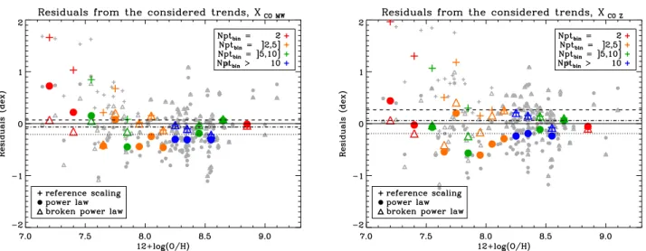
Fig. 5.Residuals (i.e., logarithmic distance) between the observed (and detected) G/D and predicted G/D from the three relations for XCO,MW(left)
and XCO,Z(right): reference scaling of the G/D with metallicity (crosses), the best power-law fit (filled circles) and the best broken power-law fit
(triangles). These residuals are shown in grey for the individual galaxies and in colour for the average residuals in each metallicity bin defined in Sect.3.1. The colours show the number of galaxies in each bin. The mean residual for all of the observed G/D values is shown by the dashed (reference scaling), dotted (power-law fit) and dash-dotted (broken power-law fit) lines for the three relations and are reported in Table1. Table 1. Parameters for the three empirical relations between the G/D
and metallicity: power law (slope of −1 and free) and broken power law for the two XCOvalues.
Parameters XCO,MWcase XCO,Zcase
Power law, slope fixed:y = a + (x − x) (“reference” scaling)
a1,2 2.21 2.21
average logarithmic distance3[dex] 0.07 0.27
Power-law, slope free:y = a + α(x − x)
a1,2 2.21 2.21
α 1.62 ± 0.34 2.02 ± 0.28
average logarithmic distance3[dex] –0.21 –0.19
Broken power law:
y = a + αH(x − x) for x > xt y = b + αL(x − x) for x ≤ xt a1,2 2.21 2.21 α1 H 1.00 1.00 b 0.68 0.96 αL 3.08 ± 1.76 3.10 ± 1.33 xt 7.96 ± 0.47 8.10 ± 0.43
average logarithmic distance3[dex] –0.06 0.06
Notes.y = log(G/D), x = 12 + log(O/H) and x = 8.69.(1)Fixed
param-eter.(2)This corresponds to the solar G/D: G/D
= 10a= 162 (Zubko
et al. 2004).(3)Derived for all of the individual galaxies, neglecting the
upper/lower limits on the G/D.
If we let αHfree in the broken power-law fit, we get similar
results within errors for αL and xt in both XCO cases. We get
αH = −0.5 ± 0.9 and αH = −1.6 ± 0.6, for XCO,MW and XCO,Z
respectively, which is coherent with a slope of –1 within errors. Note that we have imposed here that our fits go through the solar G/D determined byZubko et al.(2004). If we relax this condition (i.e., do not fix our “a” parameter in Table1), we get values of the solar G/D ranging from (G/D) = 90 to 240 within ∼60% of
the value fromZubko et al.(2004).
Now we consider the deviation from each relation by look-ing at the logarithmic distance between the observed G/D values and the G/D values predicted by each of the three relations pre-sented in Table1. This is a way to look at the residuals from the
two fits and the reference scaling, even though we did not ac-tually fit the reference trend to the G/D values. These residuals are shown in Fig.5. Average residuals in each metallicity bin defined previously are also computed. For a given point, the best relation is the one giving the residual closest to zero. From Fig.5
we have another confirmation that a reference scaling of the G/D with metallicity does not provide reliable estimates of the G/D at low metallicities 12+ log(O/H) . 8.0. We also note that, for the average residuals, the broken power law gives the residuals that are the closest to zero for nearly all of the metallicity bins in both XCO,MWand XCO,Zcases.
Even though 30% of our sample have metallicities below 1/5 Z , only seven galaxies have 12+ log(O/H) ≤ 7.5 with two
of them not detected in H (SBS1159+545 and Tol1214-277). The remaining five galaxies (IZw18, HS0822+3542, SBS0335-052, SBS1415+437 and UGC4483) are strong constraints for the broken power-law fit. These five galaxies all present broad dust SEDs peaking at very short wavelengths (∼40 µm, and ∼70 µm for HS0822+3542), indicating overall warmer dust with a wide range of dust grain temperatures, and subsequently very low dust masses; hence their high G/D. This peculiar SED shape had al-ready been noted byRémy-Ruyer et al.(2013).
Using Herschel data and a semi-empirical SED model,
Sandstrom et al.(2013) looked at the G/D in a sub-sample of
26 KINGFISH galaxies, mostly spirals. They simultaneously de-rive XCOand G/D for their sample, taking advantage of the high
spatial resolution of the KINGFISH gas and dust data. They found that the G/D for these galaxies follows the reference trend with the metallicity and shows small scatter. Their metallicity range is from 12+ log(O/H) ∼ 8.1 to 8.8 and thus these results are in agreement with our findings. Moreover the small scatter (less than a factor of 2) observed by Sandstrom et al. (2013) can be due to the fact that they are probing very similar envi-ronments. In our case we have a wide variety of morphological types represented in our sample, that results in a larger scatter (a factor of ∼5 and 3 for XCO,MWand XCO,Zrespectively for this
metallicity range). 3.4. Discussion
In the previous section, we have shown that the reference scaling relation between metallicity and G/D derived for metallicities
above 12+ log(O/H) ∼ 8.0 does not apply to objects with lower metallicity. We empirically derived a new scaling relation bet-ter described by a broken power law with a transition metallic-ity around 12+ log(O/H) ∼ 8.0, which confirms the importance of this value in low-metallicity dwarf galaxies. As mentioned in the Introduction, this reference scaling relation arises from the hypothesis that the dust formation timescale and the dust de-struction timescale behave similarly with time. Thus a possible interpretation of our results would be that the balance between formation and destruction of dust grains is altered at low metal-licity, resulting in the observed steeper trend. Dwarf galaxies are subject to an overall harder ISRF than more metal-rich envi-ronments (Madden et al. 2006). The harder UV photons travel deeper into the ISM and photoprocess dust in much deeper re-gions in the clouds limiting the accretion and coagulation of the grains. The hard ISRF also affects the dust survivability in such extreme environments, especially carbonaceous dust: the dust destruction by hard UV photons is enhanced in low-metallicity galaxies for small carbon grains (e.g.,Pilleri et al. 2012;Bocchio
et al. 2012,2013). In dwarf galaxies, dust destruction by SN
shocks is enhanced too compared to larger scale galaxies, as most of the ISM can be affected by the shock due to the small physical size of the dwarfs and the globally lower density of the ISM.
In the following paragraphs we discuss the impact of several assumptions made to estimate the G/D on our results: the dust composition, the choice of the radiation field for the dust mod-elling, and the potential presence of a submm excess in some of our dwarf galaxies.
Dust composition – Galliano et al. (2011) demonstrated that a more emissive dust grain composition compared to that of the Galaxy, using amorphous carbon instead of graphite for the carbonaceous grains, is more consistent for the low-metallicity Large Magellanic Cloud (LMC). This result has been confirmed
byGalametz et al.(2013) in a star-forming complex of the LMC
with an updated version of the SPIRE calibration8. Changing accordingly the dust composition in our low-metallicity galaxies would give lower dust masses (by a factor of ∼two to three in the case of the LMC) with more emissive dust grains and would increase the G/D by the same factor, increasing the discrepancy at low metallicities between the observed G/D and the predicted G/D from the reference scaling relation.
Radiation field – In the dust modelling, we use an ISRF with the spectral shape of the Galactic ISRF for all of our galaxies for consistency. However, the ISRF in low-metallicity dwarf galax-ies is harder, so we could wonder if this spectral shape is appro-priate for the modelling of dwarf galaxies. The shape of the radi-ation field determines the emission of out-of-equilibrium small grains. Increasing the hardness of the radiation field increases the maximum temperature the small grains can reach when they un-dergo stochastic heating. However, these very small grains only have a minor contribution to the total dust mass, and thus the assumed shape of the ISRF does not bias our estimation of the total dust mass for dwarf galaxies.
Submm excess – A submm excess has been observed in the past in several low-metallicity galaxies that current dust SED 8 This updated SPIRE calibration from September 2012 had the effect
of decreasing the SPIRE flux densities by about 10% compared to the Galliano et al.(2011) study.
models are unable to fully explain (Galliano et al. 2003,2005;
Dumke et al. 2004;Bendo et al. 2006;Zhu et al. 2009;Galametz
et al. 2009,2011;Bot et al. 2010;Grossi et al. 2010). Several
hy-potheses have been made to explain this excess among which the addition of a very cold dust (VCD) component in which most of the dust mass should reside. This VCD component would be in the form of very dense clumps in the ISM (Galliano et al. 2003,
2005). Taking this additional VCD component into account in the DGS and KINGFISH galaxies presenting a submm excess can result in a drastic increase of the dust mass and thus in a lower G/D. However,Galliano et al.(2011) showed for a strip of the LMC that the submm excess is more significant in the diffuse regions, possibly in contradiction with the hypothesis of very cold dust in dense clumps. Other studies have suggested an enhanced fraction of very small grains with high emissivity
(Lisenfeld et al. 2002;Dumke et al. 2004;Bendo et al. 2006;Zhu
et al. 2009), “spinning” dust emission (Ysard & Verstraete 2010)
or emission from magnetic nano-particles (Draine & Hensley 2012) to explain the submm excess. Meny et al. (2007) pro-posed variations of the optical properties of the dust with the temperature which results in an enhanced emission of the dust at submm/mm wavelengths.Galametz et al.(2013) demonstrated that an amorphous carbon dust composition did not lead to any submm excess in the LMC. This alternative dust composition is thus also a plausible explanation for the submm excess. As for the discussion on the dust composition, using dust masses esti-mated with amorphous carbon grains for galaxies presenting a submm excess would result in an increase of a factor of ∼2 for the G/D of these galaxies.
4. Chemical evolution models
Chemical evolution models, under certain assumptions, can pre-dict a possible evolution of the G/D as metallicity varies in a galaxy. For example, in the disk of our Galaxy, chemical evo-lution models predict this “reference” scaling of the G/D with the metallicity (Dwek 1998). We consider three different mod-els here, fromGalliano et al.(2008),Asano et al.(2013a) and
Zhukovska(2014) to interpret our data. However, we have to
keep in mind during this comparison that, since we do not know the ages of these galaxies and that the same metallicity can be reached at very different times by different galaxies, our sample cannot be considered as the evolution (snapshots) of one single galaxy.
4.1. A simple model to begin with
Galliano et al.(2008) developed a one-zone single-phase
chem-ical evolution model, based on the model byDwek(1998). They consider a closed-box model where the evolution of the dust con-tent is regulated by balancing dust production by stars and dust destruction by star formation and SN blast waves. They assume full condensation of the elements injected by Type II supernovae (SNII) into dust and instantaneous mixing of the elements in the ISM. The model is shown in Fig.6 for various SN destruction efficiencies as the dark grey zone.
Two things can be noticed from Fig. 6. First, the model is fairly consistent with the observed G/D at high metallicities within the scatter, and down to metallicities ∼0.5 Z . Second,
the model does not work at low metallicities and systematically underestimates the G/D. This has already been noted byGalliano
et al.(2008) for their test sample of galaxies and was attributed to
the very crude assumptions made in the modelling, especially the instantaneous mixing of the SNII elements in the ISM. Another
Fig. 6.G/D as a function of metallicity for the 2 values of XCO: XCO,MW(left) and XCO,Z(right) with the chemical evolution model ofGalliano
et al.(2008). The colours and symbols are the same as for Fig.4. The dark grey stripes show the range of values from theGalliano et al.(2008) chemical evolution model. The black dashed line represents the reference scaling of the G/D with metallicity (not fit to the data). The black dotted and dash-dotted lines represent the best power-law and best broken power-law fits to the data.
strong simplifying assumption made byGalliano et al.(2008) is that they did not take into account dust growth in the ISM as they assume full condensation of the grains. In the Galaxy, the typical timescale for dust formation by stars has been shown to be larger than the typical timescale for dust destruction (Jones &
Tielens 1994;Jones et al. 1996). Because we still observe dust
in the ISM, we need to reach equilibrium between formation and destruction of the dust grains, either via high SN yields or dust growth processes in the ISM. In the following sections we thus look at models including dust growth in the ISM.
4.2. Including dust growth in the ISM
Asano et al.(2013a) propose a chemical evolution model, based
on models fromHirashita(1999) andInoue(2011), taking into account the evolution of the metal content in the dust phase in addition to the evolution of the total amount of metals. The dust formation is regulated by asymptotic giant branch (AGB) stars, SNII and dust growth, via accretion, in the ISM. The dust is de-stroyed by SN shocks. Inflows and outflows are not considered (closed-box model) and the total mass of the galaxy is constant and set to 1010 M
. Metallicity and age dependence of the
vari-ous dust formation processes are taken into account.Asano et al.
(2013a) show that dust growth in the ISM becomes the main
driver of the dust mass evolution, compared to the dust formation from metals produced and ejected into the ISM by stars, when the metallicity of the galaxy exceeds a certain “critical” metal-licity. This critical metallicity increases with decreasing star for-mation timescale9.Asano et al.(2013a) show that dust growth
via accretion processes in the ISM is regulated by this critical metallicity over a large range of star formation timescales (for τSF = 0.5–5–50 Gyr). After reaching this critical metallicity
the dust mass increases more rapidly, boosted by dust growth processes, before saturating when all of the metals available for dust formation are locked up in dust. The metallicity at which 9 The star formation timescale, τ
SF, is defined by the timescale during
which star formation occurs: τSF= (MISM)/SFR, where SFR is the star
formation rate (see Eq. (5) of Asano et al. 2013a). This is not to be mixed with the timescale, τ, in exponentially decaying star formation histories going as exp−(t/τ).
this saturation occurs thus also depends on the critical metallic-ity, which in turn depends on the star formation history of the galaxy.
Figure 7 shows the models of Asano et al. (2013a) (for τSF= 0.5–5–50 Gyr) overlaid on the observed G/D values. The
models were originally on an arbitrary scale and they are thus normalised at the (G/D) value. We assume an error on this value
of ∼60%, from the range of values determined from the fits in Sect.3.3, to have a tolerance range around the model (shown by the shaded grey area in Fig.7). The three models show similar evolution with metallicity and indeed are homologous to each other when normalised by their respective critical metallicities (see Fig. 3 ofAsano et al. 2013a). We clearly see the influence of the critical metallicity on the dust mass evolution: at low metal-licities the range of possible G/D values (illustrated by the grey area in Fig.7) becomes wider around 12+ log(O/H) ∼ 7.2–7.3 before narrowing down around 12+ log(O/H) ∼ 8.6. This broad-ening is due to the fact that in this range of metallicities, galaxies with high star formation timescales have already reached their critical metallicity and have a rapidly increasing dust mass (and thus a low G/D at a given metallicity), compared to galaxies with lower star formation timescales which have not yet reached this critical metallicity and with a dust mass still regulated by stars (thus with a higher G/D at the same metallicity). Galaxies with high star formation timescales then reach saturation at moder-ate metallicities as they started their “active dust growth” phase at a lower critical metallicity (i.e., earlier in their evolution), while, at the same metallicity, galaxies with low star formation timescales are still in the “active dust growth” phase. Then when these galaxies also reach saturation, because the dust growth in the ISM becomes ineffective, the range of possible G/D values narrows down.
From Fig.7we see that the models fromAsano et al.(2013a) are consistent with the G/D from both XCOvalues.We note that
below 12+ log (O/H) ∼ 7.5, even the τSF = 50 Gyr model does
not agree anymore with the reference scaling of the G/D with metallicity (and below 12+ log(O/H) ∼ 8.0 for τSF = 5 Gyr).
The other two empirical relations (our best power-law and bro-ken power-law fits) are consistent with the models of Asano
et al. (2013a) within the considered metallicity range: from
Fig. 7.G/D as a function of metallicity for the 2 values of XCO: XCO,MW(left) and XCO,Z(right) with the chemical evolution model ofAsano et al.
(2013a). The symbols are the same as for Fig.4. The colours delineate ranges in star formation timescales τSF. The model fromAsano et al.
(2013a) is overlaid on the points for various τSF= 0.5 (red), 5 (blue), 50 (purple) Gyr. The black dashed line represents the reference scaling of
the G/D with metallicity (not fit to the data). The black dotted and dash-dotted lines represent the best power-law and best broken power-law fits to the data.
Asano et al.(2013a) models, our best broken power-law fit may
overestimate the G/D for 12 + log(O/H) ≤ 7.0. However,Izotov
et al.(2012) recently suggested that there seems to be a
metal-licity floor around 12+ log(O/H) ∼ 6.9, below which no galaxies are found in the local Universe, as already proposed byKunth &
Sargent(1986). Thus our metallicity range is close to being the
largest achievable in the local Universe as far as low metallicities are concerned.
The galaxies from the DGS, KINGFISH and G11 samples are colour coded in Fig.7by an approximation of their star for-mation timescale τSF, estimated from τSF= (Mgas+ Mdust)/SFR,
where the SFR have been estimated from LTIR (obtained by
integrating over the modelled SEDs between 1 and 1000 µm, Rémy-Ruyer et al., in prep.). The τSF values are roughly
con-sistent with the models fromAsano et al.(2013a). The median value of τSF is ∼3.0 (XCO,MW) and 5.5 (XCO,Z) Gyr, but with a
large dispersion of ∼20 Gyr around this value. As the models
fromAsano et al.(2013a) encompass most of the observed G/D
values, the dispersion seen in the G/D values can be due to the wide range of star formation timescales in the considered galax-ies. This is consistent with the large dispersion in the approxi-mated star formation timescales in our sample.
InAsano et al.(2013a), the star formation is assumed to be
continuous over the star formation timescale. However, star for-mation histories of many dwarf galaxies derived from colour-magnitude diagrams reconstruction show distinct episodes of star formation separated by more quiescent phases (e.g.,Tolstoy
et al. 2009, and references therein). For example, Legrand
et al. (2000) suggested for IZw18 a star formation history
made of bursts of star formation in between more quiescent phases, following the suggestion of Searle & Sargent (1972). Episodic star formation histories have also been suggested in Nbody/smoothed particle hydrodynamics simulations of dwarf galaxy evolution (e.g., Valcke et al. 2008; Revaz & Jablonka 2012). As we saw that the scatter in Fig.7 seems to be due to the range of star formation timescales probed by our sample, and assuming a continuous star formation, we thus need to con-sider the influence of the continuous vs. episodic star formation modes.
4.3. Episodic versus continuous star formation
In the following we compare the observationally derived G/D with results of dust evolution models in dwarf galaxies with episodic star formation history fromZhukovska(2014). These models were originally introduced to study the lifecycle of dust species from different origins in the Solar neighbourhood
(Zhukovska et al. 2008). The model of Zhukovska (2014) is
based on the Zhukovska et al. (2008) model that has been adapted to treat dwarf galaxies, specifically by considering episodic star formation. InZhukovska(2014), the equations de-scribing the evolution of the galaxy are now normalised to the total galactic masses Mtot(instead of surface densities) because
dwarf galaxies are smaller in size and thus assumed to have a well-mixed ISM. As inZhukovska et al.(2008), the modelled dwarf galaxy is formed by gas infall starting from Mtot = 0
and reaches its total mass Mtot on the infall timescale. The
as-sumed value of the infall timescale inZhukovska(2014) is set to a much shorter value for dwarf galaxies than for the Solar neighbourhood model. Since the G/D is the ratio of the gas and dust masses, it does not depend on the normalisation by the total mass Mtot, and is determined by the star formation history and
infall timescale. We refer the reader toZhukovska(2014), for more details on the modelling.
Similarly to the models from Asano et al. (2013a),
Zhukovska(2014) include dust formation in AGB stars, SN II
and dust growth by mantle accretion in the ISM. The main dif-ference between these models resides in the treatment of dust growth.Zhukovska(2014) assume a two-phase ISM consisting of clouds and an intercloud medium, where clouds are charac-terised by temperature, density, mass fraction, and lifetime. Dust growth by accretion in their model takes place only in the dense gas and also critically depends on the metallicity (seeZhukovska
2008).
In this paper, we consider three models from Zhukovska
(2014), which differ only in duration and intensity of the star formation bursts. All of the models consider six bursts of star formation starting at instants t= 0.5, 1, 2, 5, 7, and 11 Gyr. In the first and the second model, the burst duration is 50 Myr and 500 Myr, respectively, and the τSFduring bursts is 2 Gyr. The
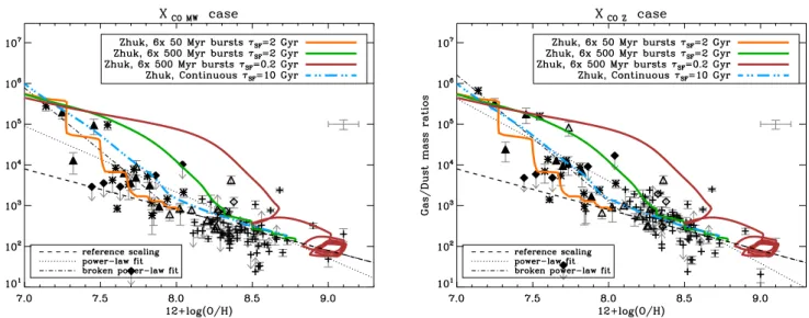
Fig. 8.G/D as a function of metallicity for the 2 values of XCO: XCO,MW(left) and XCO,Z(right) with the chemical evolution model ofZhukovska
(2014). The symbols are the same as for Fig.4. The model fromZhukovska(2014) is shown for various star formation histories: episodic with 6 bursts of 50 Myr and star formation timescale of τSF = 2 Gyr (orange), episodic with 6 bursts of 500 Myr and τSF= 2 Gyr (green), episodic
with 6 bursts of 500 Myr and τSF = 0.2 Gyr (more intense star formation, brown) and continuous with a star formation timescale τSF= 10 Gyr
(cyan dash-3 dots line). The black dashed line represents the reference scaling of the G/D with metallicity (not fit to the data). The black dotted and dash-dotted lines represent the best power-law and best broken power-law fits to the data.
second model is typical of a low-metallicity dwarf galaxy. In the third model, the burst duration is 500 Myr but the value of τSFis
much shorter, 0.2 Gyr. During the quiescence phases τSFis set
to be 200 Gyr. We also consider a model with continuous star formation on a 10 Gyr timescale, for comparison. In all of the models, the infall timescale is 0.3 Gyr and there are no galactic outflows. The initial metallicity of the infalling gas is set to be 10−4with SNII like enhanced [α/Fe] ratio.
The models fromZhukovska(2014) are presented in Fig.8
and reproduce the broadening of the observed G/D values at low metallicities (12+ log(O/H) . 8.3), and also converge around 12+ log(O/H) ∼ 7.2, similar to the models of continuous star for-mation ofAsano et al.(2013a). Note how the star formation his-tory impacts the shape of the modelled G/D: the most extreme G/D values are obtained by the three models with episodic bursts of star formation. For the model with more intense star forma-tion (brown curve in Fig.8), 12+ log(O/H) = 8.6 is reached dur-ing the first burst, and very high values of the G/D are quickly reached, up to two orders of magnitude above the reference scaling relation at moderate metallicities (12+ log(O/H) ∼ 8.2– 8.3). It also presents an interesting scatter of G/D values near 12+ log(O/H) = 9.0 that is due to dust destruction during the SF bursts, and consistent with the scatter predicted by the
Galliano et al.(2008) model (see Fig.9). The fact that the
low-metallicity slope of the broken power law is consistent with the continuous star formation model at low metallicities for the XCO,Z case indicates that this broken power law can provide a
fairly good empirical way of estimating the G/D for a given metallicity.
4.4. Explaining the observed scatter in G/D values
Figure9shows the three models overlaid on the observed G/D values. The models from Asano et al.(2013a) andZhukovska
(2014) provide trends that are consistent with each other and with the data and its scatter. More dust observations of extremely low-metallicity galaxies with 12+ log(O/H) < 7.5 are nonethe-less needed to confirm this agreement between the models and the data at very low metallicities. The model ofGalliano et al.
(2008) fails to reproduce the observed G/D at low metallicities,
but provides a good complement to explain the scatter seen at high metallicities, consistent with the predictions of the third bursty model byZhukovska(2014). We thus conclude that the observed scatter at low metallicities in the G/D values is due to the wide variety of environments we are probing, and especially to the different star formation histories. The observed scatter at higher metallicity seems to be due to different timescales for dust destruction by SN blast waves in the different environments and to the efficiency of dust shattering in the ISM.
We investigated here two different parameters to explain the scatter in the G/D values: star formation histories and efficiency of dust destruction, but other processes could also give rise to the observed scatter. In our dust modelling we allow the mass fraction of small grains compared to big grains to vary from galaxy to galaxy (controlled by the fvsg parameter), to account
for potential variations in the grain size distribution. This had al-ready been done in one low-metallicity galaxy byLisenfeld et al.
(2002). On the theoretical side,Hirashita & Kuo(2011) showed that the dust grain size distribution can have an important im-pact on the dust growth process in the ISM by regulating the grain growth rate. They also showed that the critical metallicity mentioned in Sect.4.2, for which grain growth becomes dom-inant, also depends on the grain size distribution. Additionally the grain size distribution varies as the galaxy evolves and this evolution is controlled by different dust formation processes at different ages (Asano et al. 2013b). Thus the observed scatter can also be due to variations of the grain size distribution be-tween the galaxies, the effect of which can be related to the star formation history.
As discussed in Sect.3.4, we use a dust model with the dust composition and optical properties representative of dust in the Milky Way for all of the galaxies. Another explanation for the scatter seen at all metallicities could be that the dust composition in fact varies between the galaxies, leading to large variations in the emissivity of the dust grains (Jones 2012). This would then imply dust masses relatively similar at a given metallicity but large variations in the emissivity properties of dust from one galaxy to another. With our fixed emissivity (due to our fixed dust composition in our dust model) this effect would be seen