HAL Id: cea-02320612
https://hal-cea.archives-ouvertes.fr/cea-02320612
Submitted on 18 Oct 2019
HAL is a multi-disciplinary open access
archive for the deposit and dissemination of
sci-entific research documents, whether they are
pub-lished or not. The documents may come from
teaching and research institutions in France or
abroad, or from public or private research centers.
L’archive ouverte pluridisciplinaire HAL, est
destinée au dépôt et à la diffusion de documents
scientifiques de niveau recherche, publiés ou non,
émanant des établissements d’enseignement et de
recherche français ou étrangers, des laboratoires
publics ou privés.
superbubble
T. Joubaud, I. A. Grenier, J. Ballet, J. D. Soler
To cite this version:
T. Joubaud, I. A. Grenier, J. Ballet, J. D. Soler. Gas shells and magnetic fields in the Orion-Eridanus
superbubble. Astronomy and Astrophysics - A&A, EDP Sciences, 2019, 631, pp.A52.
�10.1051/0004-6361/201936239�. �cea-02320612�
Astronomy
&
Astrophysics
https://doi.org/10.1051/0004-6361/201936239© T. Joubaud et al. 2019
Gas shells and magnetic fields in the Orion-Eridanus superbubble
T. Joubaud
1, I. A. Grenier
1, J. Ballet
1, and J. D. Soler
21Laboratoire AIM, CEA-IRFU/CNRS/Université Paris Diderot, Département d’Astrophysique, CEA Saclay,
91191 Gif sur Yvette, France
e-mail: [email protected]; [email protected]
2Max-Planck-Institute for Astronomy, Königstuhl l17, 69117 Heidelberg, Germany
e-mail: [email protected]
Received 4 July 2019 / Accepted 22 August 2019
ABSTRACT
Aims. The Orion-Eridanus superbubble has been blown by supernovae and supersonic winds of the massive stars in the Orion OB
associations. It is the nearest site at which stellar feedback on the interstellar medium that surrounds young massive clusters can be studied. The formation history and current structure of the superbubble are still poorly understood, however. It has been pointed out that the picture of a single expanding object should be replaced by a combination of nested shells that are superimposed along the line of sight. We have investigated the composite structure of the Eridanus side of the superbubble in the light of a new decomposition of the atomic and molecular gas.
Methods. We used HI21 cm and CO (J = 1−0) emission lines to separate coherent gas shells in space and velocity, and we studied
their relation to the warm ionised gas probed in Hαemission, the hot plasma emitting X-rays, and the magnetic fields traced by dust
polarised emission. We also constrained the relative distances to the clouds using dust reddening maps and X-ray absorption. We applied the Davis–Chandrasekhar–Fermi method to the dust polarisation data to estimate the plane-of-sky components of the magnetic field in several clouds and along the outer rim of the superbubble.
Results. Our gas decomposition has revealed several shells inside the superbubble that span distances from about 150–250 pc. One
of these shells forms a nearly complete ring filled with hot plasma. Other shells likely correspond to the layers of swept-up gas that is compressed behind the expanding outer shock wave. We used the gas and magnetic field data downstream of the shock to derive the shock expansion velocity, which is close to ∼20 km s−1. Taking the X-ray absorption by the gas into account, we find that the hot plasma
inside the superbubble is over-pressured compared to plasma in the Local Bubble. The plasma comprises a mix of hotter and cooler gas along the lines of sight, with temperatures of (3–9) and (0.3 − 1.2) × 106K, respectively. The magnetic field along the western and
southern rims and in the approaching wall of the superbubble appears to be shaped and compressed by the ongoing expansion. We find plane-of-sky magnetic field strengths from 3 to 15 µG along the rim.
Key words. ISM: clouds – ISM: bubbles – ISM: magnetic fields – solar neighborhood – local insterstellar matter
1. Introduction
The Orion-Eridanus superbubble is the nearest site of active high-mass star formation. It has been studied in particular to investigate the feedback of these stars on the interstellar medium. Together with supernovae and stellar winds, the intense UV stellar radiation has carved a 200 pc wide cavity that is filled with low-density ionised gas and expands into the interstellar medium. The material that was initially present was swept up and compressed to form a shell of neutral gas, the near wall of which may be as close as 180 pc from the Sun (Bally 2008). The boundary between the ionised gas and the neutral shell can be seen in Hαemission that traces the recombination of ionised
hydrogen. The Hαemission that is detected in the region is
dis-played in Fig.1. This figure features the HIIregion λ Orionis,
the bright crescent of Barnard’s Loop close to the Orion A and B molecular clouds, and the arcs of the Eridanus Loop to the west. The westernmost arc nicely delineates the outer rim of the superbubble, but the origin of the brightest vertical arc, called Arc A by Johnson(1978), is still debated. It may come from a shell inside the superbubble or from the superposition of separate structures along the line of sight.Pon et al.(2014) summarised arguments in favour and against the association of
Arc A with the superbubble based on several tracers and methods, but did not firmly conclude. They mentioned that the molecular cloud identified as MBM 18 (for Magnani, Blitz and Mundi, near αJ2000=60.◦6, δJ2000=1.◦3) byMagnani et al.(1985)
coincides in direction and tentatively in velocity with Arc A. The detection of dust reddening fronts in the PanSTARRS-1 stellar photometric data place MBM 18 within 200 pc from the Sun (Zucker et al. 2019). No significant reddening is found beyond 500 pc in this direction; this strengthens the association between Arc A and the superbubble.
The Hα emission has also been used to determine the outer
boundaries of the superbubble. Whereas it appears rather clearly defined on the western side, it had been thought that the east-ern boundary was Barnard’s Loop untilOchsendorf et al.(2015) pushed the limit farther out to a fainter feature beyond the extent of Fig. 1. The authors argued that the dusty shell of Barnard’s Loop was not optically thick enough to absorb all ionising photons from the Orion OB1 association. These pho-tons leak through to a more distant wall that is identified in gas velocity and as a faint Hα filament closer to the Galactic plane.
Barnard’s Loop is part of a closed bubble that may be driven by a supernova and expands inside the superbubble. The other shells (GS206-17+13, Orion Nebula) and the complex history
A52, page 1 of19
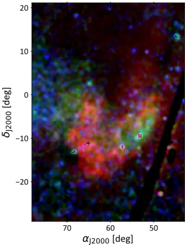
Fig. 1.Hαintensity map of the Orion-Eridanus superbubble based on
VTSS, SHASSA, and WHAM data. The dashed line traces the con-tour of the analysed region. The white labels on the left-hand side show the key Hα features towards Orion. In the analysed region, the black
contours delineate the main HIshells we identify in Sect.3: the north rim (N), south loop (S), east shell (E), and west rim (W). The line of constant Galactic latitude b = −8◦in the upper left corner indicates the
orientation of the Galactic plane.
of λ Orionis (possibly a supernova remnant cavity that has later been filled by the HIIregion around the OB association, Dolan & Mathieu 2002) ledOchsendorf et al.(2015) to change the simple picture of a single expanding object to a more com-plex combination along the line of sight of evaporating clouds and nested shells filled with X-ray emitting hot gas at different temperatures (Snowden et al. 1995).
On the plane of the sky, the elongated bubble extends from beyond Orion up to the Eridanus Loop, but its overall orientation is still uncertain. Absorption line measurements (Welsh et al. 2005) and dust extinction data from Gaia and the Two Micron All-Sky Survey (2MASS;Lallement et al. 2018) support a close end towards Eridanus (southwest) and a far end beyond Orion (east), whereas models of a single shock front expanding in an exponentially stratified interstellar medium (ISM) fit the Hαdata
better, with the Orion side being closer than the Eridanus side (Pon et al. 2016). The models cannot accommodate the com-posite structure of the superbubble, however, which has likely evolved in space and time from near to far along the blue stream of massive stars identified byPellizza et al.(2005) andBouy & Alves(2015) between us and the Orion clouds.
We have performed a multi-wavelength analysis of the gas and cosmic-ray content of the Eridanus side of the superbub-ble, which we present in a series of three papers. This paper focuses on the composite structure of atomic and molecular gas shells and on their relation to the hot ionised gas, the recom-bination fronts, and the magnetic field structure. The second paper (Joubaud et al., in prep., hereafter Paper II) explores the cosmic-ray flux that pervades the gas shells. The third paper (Joubaud et al., in prep.) studies the gas mass found at the
transition between the atomic and molecular phases and in the CO-bright parts, as well as the evolution of the dust emission opacity (per gas nucleon) across the different gas phases. The third paper also studies the small molecular cloud of MBM 20, also called Lynd dark nebula (LDN) 1642, that might be com-pressed at the edge of the Local and/or Eridanus bubbles, near αJ2000=68.◦8, δJ2000=−14.◦2.
Here we investigate the composite structure of the Orion-Eridanus superbubble in the light of a new separation of the HIgas in position and velocity. We find new shells and study their relation to dust reddening fronts, Hαand X-ray emissions,
and the magnetic field orientation derived from dust-polarised emission. We also use the HI line information to estimate the
magnetic field intensity in several parts of the superbubble. The paper is structured as follows. Data are presented in Sect.2. The separation of the HIand CO clouds and their
rela-tions in velocity, distance, and to known entities are discussed in Sect.3. We study the X-ray emission and derive the emitting plasma properties in Sect4. We probe the magnetic field ori-entation and strength in Sect.5, before we conclude in Sect.6. We present X-ray optical depth maps in AppendixAand the two methods we used to derive the angular dispersion of the magnetic field in AppendixB.
2. Data
We have analysed the eastern part of the superbubble towards the Eridanus constellation. It extends from 43◦to 78◦in right
ascen-sion and from −29◦to 21◦in declination, as shown in Fig.1. We
masked two 5◦wide areas on the western and eastern sides of the
region to avoid complex gas distributions in the background. All maps are projected onto the same 0.25◦spaced Cartesian grid.
2.1. Ionised gas
Warm ionised gas is visible through Hαemission. It is displayed
in Fig. 1 using the data of Finkbeiner(2003). This is a com-posite map of the Virginia Tech Spectral line Survey (VTSS), the Southern H-Alpha Sky Survey Atlas (SHASSA), and the Wisconsin H-Alpha Mapper (WHAM). The velocity resolution is 12 km s−1and the spatial resolution is 60(full width at half
maximum, FWHM).
2.2. HIand CO emission line data
We used the 1602 resolution HI4PI survey (HI4PI Collaboration
2016), with a velocity resolution of 1.49 km s−1in the local
stan-dard of rest (LSR). We selected velocities between −90 and 50 km s−1 to exclude the HI emission from the high-velocity
clouds that lie in the hot Galactic corona far behind the local medium we are interested inWakker et al.(2008).
In order to trace the molecular gas, we used the 8.05 resolution 12CO (J = 1−0) observations at 115 GHz from the
moment-masked CfA CO survey (Dame et al. 2001;Dame & Thaddeus 2004). We completed this dataset with the CO observations of the MBM 20 cloud obtained with the Swedish-ESO Submillime-tre Telescope (SEST) that were kindly provided byRusseil et al.
(2003). 2.3. X-ray data
In order to study the hot-gas content of the superbubble, we used data from the Roentgen satellite (ROSAT) X-ray all-sky survey (Snowden et al. 1994). The spatial resolution is about 3000
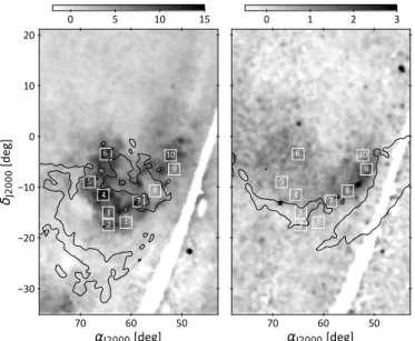
Fig. 2.Maps of the north rim, south loop, east shell, west rim, MBM 20, Eridu cirrus, Cetus, and North Taurus components in HIcolumn density,
NHIfor a spin temperature of 100 K, and in CO line intensity, WCO.
the 0.25 keV band, spanning from 0.11 to 0.284 keV at 10% of peak response (R1+R2), the 0.75 keV band from 0.44 to 1.2 keV (R4+R5), and the 1.5 keV band from 0.7 to 2 keV (R6+R7). The exposure over the analysed region varies between 0 and 600 s, therefore we masked out the underexposed zones with exposure times below 80 s. They appear as white stripes in our inten-sity maps. Even though we used count rates that take striped variations in the exposure map into account, we caution that sys-tematic biases remain in the survey calibration. They appear as striped enhancements or diminutions in count rates that cross the analysis region roughly parallel to the underexposed stripes. We re-sampled the maps onto our 0.◦25 grid and have compared the
two low-energy count rate maps with those ofSnowden et al.
(1994). 2.4. Dust data
We used the 3D dust reddening maps of Green et al. (2018). These maps span three quarters of the sky (δ & −30◦) and are
based on the stellar photometry of 800 million stars from Pan-STARRS 1 and 2MASS. The authors divided the sky into pixels containing a few hundred stars each. This results in a map with pixel sizes that vary from 3.04 to 550.
The polarisation data, that is, the total intensity and the Q and U Stokes parameters, come from the Planck 353 GHz 2018 polarisation data with an original angular resolution of 50 (Planck Collaboration XII 2019). To enhance the
signal-to-noise ratio, we smoothed the maps and their covariances to 400 resolution (FWHM) and downgraded the healpix maps to
Nside=512.
3. HIand CO cloud separation
3.1. Velocity decomposition
Following the method developed by Planck Collaboration Int. XXVIII(2015), we decomposed the HI and CO velocity
spec-tra into individual lines and used this information to identify and separate eight nearby cloud complexes that are coherent in position and in velocity. We thus fitted each HI or CO
spec-trum as a sum of lines with pseudo-Voigt profiles that combine a Gaussian and a Lorentzian curve that share the same mean and standard deviation in velocity. The Lorentzian part of the profile can adapt, if necessary, to extended line wings that are broad-ened by velocity gradients within the beam. The prior detection of line peaks and shoulders in each spectrum provided a limit
on the number of lines to be fitted as well as initial guesses for their central velocities. We improved the original method by tak-ing the line information of the neighbourtak-ing spectra into account for each direction in order to better trace merging or fading lines. The fits yield small residuals between the modelled and observed spectra, but in order to preserve the total intensity that is recorded in each spectrum, we distributed the residuals among the fitted lines according to their relative strength in each channel. 3.2. HIand CO components
The 3D (right ascension, declination, and central velocity) dis-tribution of the peak temperatures of the fitted lines showed that the data can be partitioned into several entities that are depicted in NHIcolumn densities and in WCOintensities in Fig.2. Some
were detected in both HI and CO emission lines, such as the
north rim, south loop, east shell, Cetus, North Taurus, and MBM 20. The others were only seen in the HIdata, such as the west
rim and Eridu cirrus. To construct these maps, we defined 3D boundaries in right ascension, declination, and velocity for each component. The velocity range for each cloud is presented in Table1. We selected the fitted lines with central velocities falling within the appropriate velocity interval, depending on the (α, δ) direction, and we integrated their individual profiles in velocity. The resulting maps were then re-sampled into the 0.◦25 spaced
Cartesian grid of the analysed region.
In order to investigate the effect of the unknown HIoptical
depth, we derived all the NHImaps for a set of uniform spin
tem-peratures (100, 125, 200, 300, 400, 500, 600, 700, and 800 K) and for the optically thin case.Nguyen et al.(2018) have recently shown that a simple isothermal correction of the emission spec-tra with a uniform spin temperature reproduces the more precise HIcolumn densities that are inferred from the combination of emission and absorption spectra quite well. Their analysis fully covers the range of column densities in the Eridanus region. All the figures and results presented here were derived for a spin temperature of 100 K. This choice comes from the best-fit mod-els of the γ-ray data and of the dust optical depth at 353 GHz; they are detailed in Paper II. This choice has no effect on cloud separation. Compared with the optically thin case, the correction increases the highest column densities (>1.5 × 1021cm−2) of the
thickest cloud of the north rim by 40%. The other clouds are more optically thin.
As we discuss in this paper, some structures are likely asso-ciated with the superbubble (north rim, south loop, east shell, and west rim), while the others are foreground (MBM 20), back-ground (Cetus, North Taurus) or side (Eridu) clouds. The north rim component gathers elements that have previously been iden-tified as independent features, such as the MBM 18 (L1569) molecular cloud at a distance of 155+3
−3 pc (Zucker et al. 2019)
and the G203-37 cloud towards (66◦, −9◦) thatSnowden et al.
(1995) placed midway through the hot superbubble cavity. Other MBM clouds of interest are listed in Table1. We did not push the partition of the north rim farther because the lines are con-fused in space and velocity, despite the sparse decomposition of the spectra into individual lines. We reached the same conclu-sion using another decomposition method called the regularized optimization for hyper-spectral analysis (ROHSA1). The analysis kindly provided by Antoine Marchal recovered the same struc-tures for the east shell and west rim. This supports our separation. However, it also struggled to identify individual entities in the complex distribution in the northern part. We therefore preferred to keep the north rim as a single component for our analyses.
1 https://antoinemarchal.github.io/ROHSA/index.html
Fig. 3.Spatial distribution of the peak temperatures of the fitted HIlines (grey scale) for different slices in central velocity (indicated in km s−1
in the lower left corner of each plot). The red circle highlights the outer shell that is visible at +9 km s−1.
Part of the analysed region overlaps the anticentre region studied byRemy et al.(2017), who used a similar method to sep-arate gas clouds. We recovered the same structures in velocity and space in the overlap region: their North Taurus and Cetus components, with minor differences due to their use of data with higher velocity resolution from the Galactic Arecibo L-Band feed array (GALFA) in those directions. Their South Taurus complex mainly contributes to the north rim in our analysis. Their main Taurus complex only marginally overlaps with our region. The bulk of this cloud lies beyond our analysis boundary and is not discussed here.
3.3. Relative motions in the superbubble
The distribution in position and velocity of the HI line
cores that result from the line decomposition allows us to resolve the relative motions that subtend this complex environ-ment. In the original data cubes, the bulk motions are often
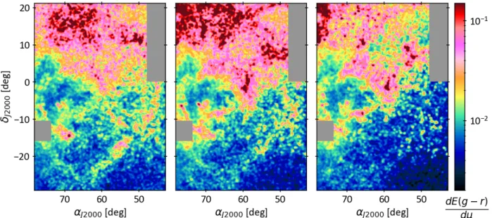
Fig. 4.Maps of the dust reddening per unit distance modulus, dE(g−r)
dµ , showing the morphology of dust fronts at distances of 200 pc (left), 320 pc
(middle), and 400 pc (right). The maps are smoothed by a 0.◦4 Gaussian kernel for display.
buried in the overlap of the broad wings of the HI lines. We
display slices through the HI line distributions for specific velocities in Fig.3. The central velocities of the HIlines
associ-ated with the superbubble range from −15 to +18 km s−1. This
range compares with the [−25, +5] km s−1 range derived by
Reynolds & Ogden(1979) from the Hα emission. The map at
+9 km s−1exhibits a coherent circular ring that suggests that we
intercept the outer rim of the expanding shell tangentially along these lines of sight. Most of the gas at higher (receding) veloc-ities is indeed seen within the boundary of the outer rim. The slice at +4 km s−1shows another circular ring in the south that
corresponds to the rim of the south loop. The expansion veloc-ities of these two rings are in the plane of sky because we see the rims tangentially. The radial line velocities thus indicate that the bulk of the outer rim and of the south loop recede at +9 and +4 km s−1, respectively, with respect to us. This means that the
south loop approaches us with respect to the rest frame of the superbubble. The slice at −9 km s−1shows the east shell, which
approaches fast. We give evidence in Sect.4that it moves inside the superbubble.
When we exclude the internal motion of the east shell to fol-low the outer expansion, the HIline range is reduced to [−5, +19]
km s−1. With a rest frame velocity of +9 km s−1, the line data
suggest an expansion velocity of about 10–15 km s−1, which is
lower than the 40 km s−1inferred byBrown et al.(1995) from the
full extent of the HIspectra, including the line wings. It is
con-sistent with the 15–23 km s−1velocity found in H
α(Reynolds &
Ogden 1979). It also compares with the low velocity of 8 km s−1
expected from simulations (Kim et al. 2017) for a superbubble that expands in a medium with a mid-plane gas density of 1 cm−3
and a scale height of 104 pc that is powered by a supernova rate of 1 per Myr; this is close to the rate of Orion-Eridanus super-bubble (Voss et al. 2010). The simulations also show that the compressed swept-up gas behind the shock expands at slightly lower velocities than the shock itself and than the hot phase. 3.4. Dust reddening distances
In order to study the 3D gas distribution in the superbubble and to substantiate the cloud separation in velocity, we used the 3D
reddening maps ofGreen et al.(2018). They inferred a reddening profile as a function of distance modulus, µ, for each direction in the sky using the photometric surveys of Pan-STARRS 1 and 2MASS in a Bayesian approach. We located gas concentrations in distance in these profiles by searching for reddening fronts that can be identified as sharp increases in the amount of dust redden-ing per unit length. To do so, we took the derivative of their best-fit profiles for each direction in the sky. We display the derivative maps in Fig. 4 for three distances at 200, 320, and 400 pc. The west rim and MBM 20 clouds are clearly identified around 200 pc, and the north rim appears between 200 and 320 pc. The CO-bright molecular parts of the east shell are visible at 320 pc. The G203-37 cloud appears between 320 and 400 pc.
The 3D partitioning of the dust fronts was not induced by the Bayesian priors that were used to build the reddening profiles.
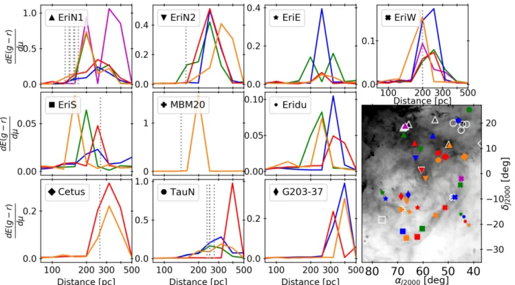
Green et al.(2018) have used broad-band photometric measure-ments of each star and have computed a probability distribution over the stellar distance and foreground dust column. They con-strained their prior on theSchlegel et al.(1998) reddening map, which is a scaled version of an optical depth map of the dust thermal emission integrated along the lines of sight, without information along the radial dimension. The spatial correlation we find between the dust maps in distance and the morphology of the clouds we isolated strengthens our confidence that the dif-ferent complexes are separated in velocity as well as in distance. We constrained the distance range to each cloud complex using the reddening front information towards several directions in each complex. Their locations are marked in Fig.5. For each direction, we selected derivative profiles within a radius of 1◦,
and we averaged those whose peak dE(g−r)dµ value exceeded 80% of the maximum. The results are shown in Fig.5. Distance ranges based on these profiles are given in Table 1 together with the velocity ranges observed in the HIdata. Table1also lists
dis-tances to MBM molecular clouds that appear to be associated in space and velocity with our cloud complexes. Their distances have been derived byZucker et al.(2019) using the same redden-ing method, but choosredden-ing individual stars.Lallement et al.(2018) constructed another 3D dust map using inversion methods and the stellar surveys of Gaia, 2MASS, and the APO Galactic Evo-lution Experiment (APOGEE) DR14. Three vertical cuts across
Fig. 5.Mean reddening per distance unit profiles towards several directions for each HIcloud. The mean is computed for each direction over selected profiles in a circle with a radius of 1◦. The map shows the pointed directions overlaid on the HIcolumn density. The different markers
correspond to the different cloud complexes, and the colours show the different directions for a given cloud. The cloud labels are north rim (EriN), west rim (EriW), east shell (EriE), south loop (EriS), and North Taurus (TauN). For clarity, we divided the north rim into its northern part (EriN1, upwards-pointing triangle), which marks the superbubble boundary, and its southern part (EriN2, downwards-pointing triangle), which overlaps the MBM 18 cloud. The white markers on the map show the MBM clouds. Their shape corresponds to the complex they are associated with. Their distances were derived byZucker et al.(2019) and are reported in the plots with grey dotted lines.
the Galactic disc towards the Galactic longitudes of 192◦, 205◦,
and 212◦ yield distances to our gas complexes that are listed in
Table1.
The different measurements in Table1indicate that most of the clouds associated with the superbubble, such as the north rim and west rim, the east shell, south loop, and MBM 20, lie at distances ranging between 150 and 250 pc. The distances and velocities we obtain for the different complexes are consis-tent with those found with NaI and CaII interstellar absorption lines towards early-type stars throughout the region (Welsh et al. 2005). We note, however, that distances based on the redden-ing information from Green et al. (2018) tend to yield higher values than towards individual stars. This is partly due to their binning in space and in log(µ), which was adapted to large-scale 3D mapping in the Galaxy, and to the lack of stars at high Galac-tic latitudes. The lower bound of our distance estimates should also be considered with care as they approach the shortest range allowing large enough stellar samples to infer the average red-dening and to recognise the shape of the cloud. Adding stars from Gaia alleviates the biases. All sets of values neverthe-less give weight to a superbubble orientation with its close end towards Eridanus.
A series of MBM clouds (MBM 16, 106, 107, 108, and 109) is associated with the north rim and more specifically with the outer rim because of their location and velocity. They gather at distances between 140 and 170 pc. The MBM 18 cloud, at a comparable distance, is also associated with the north rim in HI
and CO. Together they suggest that the broad north rim complex combines gas from the outer rim seen edge-on and face-on (see the middle right panel of Fig.3). We therefore conclude from
the synergy in distance and velocity of the north rim, south loop, and west rim that they represent the front face of the superbubble with respect to us.
Figure4also shows the G203-37 cloud at a distance between 300 and 400 pc, in agreement withSnowden et al.(1995). These authors had placed it midway through the hot superbubble cavity. The MBM 22 cloud is seen in a direction close to the rim of the south loop, and its velocity is consistent with the south loop range, but its distance of 266+30
−20 pc places it behind the south
loop. This is corroborated by the maps in Fig. 4, which show that the south loop is most conspicuous in the left (200 pc) panel and fades out at 320 pc, whereas MBM 22 appears at 320 pc and fades out at a larger distance. MBM 9 and the clouds of Cetus and North Taurus also lie outside and behind the superbubble, at distances between 250 and 400 pc. We note that the Cetus and North Taurus clouds are part of larger complexes that extend well beyond the western side of the analysed region (Remy et al. 2017).
3.5. MBM 20 and the edge of the superbubble
Inspection of relative distances in Figs. 4 and 5 suggests that MBM 20 and the closest clouds of the south loop may be interacting with the Local Bubble at about 150 pc in the pic-ture ofBurrows et al.(1993). This is consistent with the velocity configuration discussed above, where the south loop approaches us compared to the rest of the superbubble.
A clear HIand CO component in our separation corresponds
to the well-studied MBM 20 (L1642) cloud (Russeil et al. 2003). It is clearly visible in the 200 pc map of Fig. 4 at α = 68.◦8
Table 1. Distance and velocity range of the main HIclouds and the overlapping MBM clouds.
Velocity Dist.(a) Dist.(b) cloud (α, δ) MBM Dist.(c) MBM Vel.(d)
(km s−1) (pc) (pc) J2000 (pc) (km s−1) Superbubble components North rim [4, 25] [150, 400] 140 ± 40 MBM16 (49.◦8, 11.◦6) 170+2 −1± 8 7.4 170 ± 40 MBM 17(e) (55.◦2, 21.◦3) 130+2 −1± 6 7.9 MBM 107 (66.◦9, 18.◦9) 141+4 −13± 7 8.6 MBM 108 (67.◦2, 18.◦5) 143+2 −2± 7 7.6 MBM 18 (60.◦6, 1.◦3) 155+3 −3± 7 8.0 MBM 109 (67.◦9, 18.◦1) 155+10 −8 ± 7 6.6 MBM 106 (65.◦7, 19.◦5) 158+27 −10± 7 8.5 South loop [−3.8, 7.8] [150, 300] East shell [−30.8, −2.5] [200, 300] West rim [−2.5, 15.6] [150, 250] 180 ± 30 MBM 15 (48.◦2, −9.◦4) 200+27 −24± 10 4.4 210 ± 40 Other complexes MBM 20 [0, 4] [150, 250] 180 ± 40 MBM 20 (68.◦8, −14.◦2) 141+3 −2± 7 0.3 MBM 22 MBM 22 (76.◦2, −18.◦3) 266+30 −19± 13 4.5 Eridu cirrus [−13, −2] [200, 400] 210 ± 30 North Taurus [−6, 4] [250, 450] 370 ± 50( f ) MBM 13 (44.◦9, 17.◦2) 237+5 −6± 11 −5.7 MBM 11 (42.◦8, 19.◦5) 250+5 −7± 12 −6.6 MBM 12 (44.◦2, 19.◦5) 252+4 −6± 12 −5.3 MBM 14 (48.◦0, 20.◦0) 275+3 −6± 13 −2.2 Cetus [−20, −5] [250, 400] 370 ± 50( f ) MBM 9 (36.◦6, 11.◦9) 262+22 −14± 13 −13.0 G203-37 [8, 15] [300, 400] (66.◦0, −9.◦0)
Notes. (a)From the reddening front method described in this paper.(b)FromLallement et al.(2018).(c)FromZucker et al.(2019). The first errors are
statistical, and the second give the systematic uncertainties.(d)FromMagnani et al.(1985).(e)The association of MBM 17 cloud with north rim is
uncertain because of the velocity confusion in this direction.( f )It is uncertain whether the association should be with Cetus or North Taurus.
and δ = −14.◦2. Its distance of 141+3
−2 pc (Zucker et al. 2019) or
180 ± 40 pc (Lallement et al. 2018) places it near the bound-ary between the superbubble and the Local Bubble. Snowden et al.(1995) used X-ray absorption to place MBM 20 inside the Local Bubble, thus pushing the closest superbubble wall beyond 140 pc. The cometary tail of MBM 20 is visible in HI. It points to
the north-east of the compact CO cloud (see Fig.2) and extends over 10 pc (at 140 pc). It presents a velocity gradient whose tail tip moves faster away from us than the molecular head, in agree-ment with having been swept up by the expanding medium of the Local Bubble rather than by the south loop. MBM 20 may therefore lie just in front of the edge of the superbubble. We note that despite similar orientations and some overlap in direction with the east shell, the two clouds are distinct and have different velocities, as is shown in Table1.
3.6. Cloud relations to the Hαfilaments
The HIand CO structures we isolated can be compared to the
Hα intensity map. Hα line emission at 656.3 nm arises from
the recombination of an electron onto ionised hydrogen, so that the lines trace the ionised gas at the interface with colder atomic hydrogen, where the ionisation fraction is still high, but the density is also high enough for recombination to occur. Figure6displays Hα line intensity maps integrated over [−60,
−11] and [−11, 50] km s−1. We overlaid HIcontours of specific
clouds. The 12 km s−1resolution of the WHAM H
αdata prevents
detailed velocity comparisons between the HI, CO, and Hαlines,
but it can still capture interesting relations. As the neutral HI
structures surround the recombining shells with a small angu-lar offset, Fig.6 outlines a mosaic of boundaries between hot sub-bubble interiors and their colder outer shells, which are com-pressed by the hot-gas expansion (see Figs. 3 and 4 ofKrause et al. 2013).
The east shell is related to a specific Hα filament. Both
structures move inside the superbubble towards us (negative velocities) at a distance constrained by the dust to be about 300 pc. The southern part of the south loop might be associated with the Hα filament called Arc C (Johnson 1978). The round
structure of the loop in HIand Hαand its radius of ∼35 pc at a
distance of 200 pc are reminiscent of an old supernova remnant, but they may also reflect global oscillations of the hot gas in the superbubble. Such oscillations are induced by off-centred super-nova explosions in a hot cavity (Krause et al. 2014). We further discuss the origin of the loop in the next sections. The west rim is related to the Arc B filament in Hα(Johnson 1978). We see an
elongated shock wall almost edge-on, with velocity excursions of −10 to +7 km s−1about the rest velocity of +9 km s−1. The
clos-est part approaches us and is superimposed on receding parts that lie farther away. The Hαemission from the rest of the outer rim
is likely absorbed by the high gas column densities pertaining to the north rim (typical visual extinctions of 0.4–1.8 magnitudes
Fig. 6. Hα line intensity maps for two velocity ranges, [−60, −11]
(top) and [−11, 50] km s−1(bottom), overlaid with N
HI column density
and WCO emission contours outlining the different cloud components:
the east shell in HI(red, 1.5 × 1020cm−2), the west rim in HI(cyan,
4 × 1020 cm−2), the south loop in HI (green, 2.5 × 1020 cm−2), and
the north rim in CO (yellow dashed line, 1 K km s−1). The N HI and
WCO maps are smoothed with a Gaussian kernel of 0.◦28 to display
the contours. A specific north rim contour is shown in HI for
cen-tral line velocities of +9 km s−1 (dark blue dash-dotted line, 18 K). It
was smoothed with a Gaussian kernel of 1.◦5 before the contours were
computed.
up to a distance of 300 pc along the northern part of the outer rim; this is outlined in dotted contours in Fig.6. Towards the west rim, the visual extinctions range from 0.1 to 0.4 magnitudes).
The brightest Hαarc, Arc A, extends vertically in the centre
of the positive-velocity map in Fig.6. Its relation to the super-bubble is still debated; seePon et al.(2014) for a discussion that takes the proper motion and radial velocities, as well as X-ray and Hαemission and absorption studies, into account. Based on
the width and intensities of the Hα lines, these authors argued
that the Hα filaments are either elongated sheets seen
edge-on or objects that are out of equilibrium as a result of iedge-onised clouds that are compressed by shocks that currently recombine. While Arc B seems to comply with the edge-on sheet hypothesis, the situation is not clear for Arc A because of the confusion along the line of sight, the spread of Hα and HIemission over
a wide range of velocities, and absorption from atomic and dark neutral gas (see Paper II) and from molecular gas in MBM 18. As reported byPon et al.(2014), the coincidence in space and velocity between Arc A and MBM 18 tends to favour an asso-ciation of the arc with the superbubble. Figure 6 shows that the northern part of Arc A nicely follows an arc of molecular clouds belonging to the north rim component and that Arc A is partially absorbed by the dense gas in MBM 18 near αJ2000 =
60.◦6, δJ2000=1.◦3. The dust associated with the molecular arc is
visible at close distance in Fig.4, but not at 400 pc, nor beyond. The distance to Arc A is thus constrained to be between that of MBM 18 (155+3
−3pc,Zucker et al. 2019) and an upper bound
of about 400 pc. Arc A therefore likely represents an inner shell of the superbubble seen edge-on, as for the east shell.
4. X-ray emission
The Eridanus X-ray enhancement arising from diffuse hot gas has been extensively studied to constrain the properties of the hot superbubble interior and the distribution of foreground gas seen in absorption against the bright X-rays (Burrows et al. 1993;
Snowden et al. 1995;Heiles et al. 1999). We now compare the spatial distribution of the different clouds we isolated with that of the X-rays recorded in three energy bands with ROSAT, and we take advantage of our study of the total gas column densities in the atomic, dark, and molecular gas phases (see Paper II) to quantify the X-ray absorption.
Figure 7 displays the ROSAT maps recorded in the 0.11–0.284 keV (R1+R2), 0.44–1.21 keV (R4+R5), and 0.73– 2.04 keV (R6+R7) energy bands (Snowden et al. 1994). We refer to these bands below as the 0.25, 0.75, and 1.5 keV bands, respectively. Two main features have originally been identified (Burrows et al. 1993). The first, called Eridanus X-ray enhance-ment 1 (EXE1), appears in the 0.75 and 1.5 keV maps as a crescent bounded to the west by the west rim clouds, to the south by the east shell, and to the east, it extends towards Orion. Its northern extent is unknown because it is obviously heav-ily absorbed, even at 1.5 keV, by the 1.4 ×10⁵ solar masses of
gas associated with the north rim (see Fig.7). EXE1 was asso-ciated with the interior of the superbubble by Burrows et al.
(1993). The brightest part of the crescent at 0.75 keV is located between the Hα arcs A and B. This region was found to be a
small independent expanding shell in HαbyHeiles et al.(1999).
The second main feature (EXE2) is visible only at 0.25 keV, below δ = −10◦. This soft excess is obviously barred by
absorp-tion from the gas in the south loop and by the compact MBM 20 cloud, which creates a marked dip in X-rays around α = 68.◦8 and
δ =− 14.◦2. The east shell, however, leaves no obvious absorption imprint. The bright part of EXE2 that partially overlaps the south loop was first interpreted as hot gas originating from a supernova remnant or a stellar wind bubble (Burrows et al. 1993), but the absence of an OB star in this direction ledHeiles et al.(1999) to
J20
00
J20
00
Fig. 7.ROSAT intensity maps in units of 103counts s−1sr−1 in the 0.25 keV band (covering between 0.11 and 0.284 keV, left column), in the
0.75 keV band (covering between 0.44 and 1.21 keV, middle column), and in the 1.5 keV band (covering between 0.73 and 2.04 keV right column) from the all-sky survey in the top row, and the same maps corrected for the Local Bubble foreground emission and for a halo background emission in the bottom row (according to Eq. (3)). HIcolumn density contours outline different cloud complexes: the north rim absorbs X-rays at all energies and is displayed in the 1.5 keV map (at NHI= 1.5 ×1021cm−2). The west rim cloud bounds the X-ray emission at all energies and is displayed in
the 0.75 keV map (at NHI=2 × 1020cm−2). The east shell cloud bounds the southern parts of the 0.75 and 1.5 keV emissions, but does not absorb
the 0.25 keV emission. It is displayed in the 0.75 keV map (at NHI= 1.4 ×10²⁰). Additional absorption at 0.25 keV relates to the south loop (NHI=
2 ×1020cm−2) and to MBM 20. The latter is not displayed, but is visible as the dark blue spot around α = 68.◦8 and δ = −14.◦2 in the top 0.25 keV
map. For clarity, we smoothed he X-ray maps and HIcontours with a Gaussian kernel of 0.◦3 for display and maksed underexposed regions in the
ROSAT survey in white.
propose that hot gas leaks out of EXE1 at the rear of the super-bubble through a break in its shell and that the gas cools in the external ISM. Because the soft emission extends below −25◦ in
declination,Snowden et al.(1995) instead interpreted EXE2 as soft background emission arising from the million-degree gas in the Galactic halo and being shaped into a roundish feature by intervening gas absorption. We revisit the properties of EXE1 and EXE2 below.
4.1. Subtracting foreground and background emission We followed the simple slab model ofSnowden et al.(1995) and modelled the observed X-ray intensity in each energy band and
direction as
Iobs(α, δ) = ILocal Bubble+IEri(α, δ) e−τX(α,δ)+Ihaloe−τtot X(α,δ), (1)
where ILocal Bubble, IEri, and Ihalo represent the X-ray intensities
arising from the Local Bubble, the Orion-Eridanus superbub-ble, and the halo, respectively. The foreground and background emissions from the Local Bubble and the halo are assumed to be uniform. τXdenotes the X-ray optical depth of the absorbing gas
located in front of the superbubble, and τtot X denotes the total
optical depth along the line of sight.
In order to compute the X-ray optical depths, we used the NH gas column densities inferred in the different gas phases
and different cloud complexes from our combined HI, CO, dust, and γ-ray study, following the same method to map and quan-tify the amount of gas as applied earlier in other nearby regions (see Paper II, Planck Collaboration Int. XXVIII 2015; Remy et al. 2017). Snowden et al.(1995) have instead used the dust emission map at 100 µm to trace NH, but they did not
cor-rect the map for biases that have since then been found to be significant (e.g. spatial variations in dust temperature and spec-tral index (Planck Collaboration XI 2014) and the non-linear increase of the dust emissivity per gas nucleon with increas-ing NH(Planck Collaboration XI 2014;Planck Collaboration Int.
XXVIII 2015;Remy et al. 2017). We derived the optical depths from our column density maps using
τX(EX) = σ(EX,NH) × NH, (2)
with EX the X-ray band and σ the energy-band-averaged
pho-toelectric absorption cross section fromSnowden et al.(1994). For the 0.25 and 0.75 keV bands, we took an incident thermal spectrum with a temperature of 1.3 MK close to the mean colour temperature observed towards the Eridanus X-ray excesses (see below). For the 1.5 keV band, we assumed a power-law incident spectrum with an index of −2. We verified that the choice of temperature and spectral index around these values has a small effect on the result. The optical depth maps obtained for the total gas column densities τtot Xare presented in Fig.A.1for the three
energy bands.
We find that the north rim is optically thick in the lower energy bands and is still partially thick (0.5 . τtot X . 1) at
1.5 keV, which explains the northern shadows in all plots of Fig.7. Inspection of the optical depth maps for individual cloud complexes indicates that the west rim is thick at 0.25 keV, nearly so at 0.75 keV, and mostly thin (0.1 . τX.0.2) at high energy.
The south loop is thick at low energy and mostly thin in the two upper bands. The east shell is thick at low energy (1 . τX.2.5),
partially thick at 0.75 keV (0.1 . τX . 0.4), and thin at high
energy. The molecular head of MBM 20 is optically thick at low energy, nearly so at medium energy, but partially transparent at high energy.
In order to estimate upper limits to the emission from the Local Bubble in the three ROSAT bands, we studied the distri-bution of X-ray intensities versus gas column density towards a set of heavily absorbed and nearby clouds: towards MBM 20 (which is likely located at the interface between the Local Bub-ble and the Eridanus superbubBub-ble), MBM 16, MBM 109, and MBM 18. To limit the effect of noise fluctuations towards these faint regions, we calculated the minimum intensities averaged over the high-NHtot pixels in each region, at NH>7 × 1020cm−2
in the low band and NH>1.5 × 1021cm−2in the upper bands, and
we excluded pixels with X-ray point sources. We find an upper limit to the Local Bubble intensity of 4.0 × 10³ cts s−1sr−1 at
0.25 keV, which coincides with the estimate ofSnowden et al.
(1995). We find upper limits of 0.8 × 10³cts s−1sr−1at 0.75 keV
and 1.1 × 10³cts s−1sr−1at 1.5 keV, which are consistent towards
the four clouds.
In order to estimate the background halo intensities in direc-tions away from the superbubble, we corrected the observed X-ray maps for the Local Bubble emission and for the total gas absorption using Ihalo=(Iobs− ILocal Bubble) e+τtot X. We
aver-aged the intensities over the low-absorption region at 50◦≤ α ≤
60◦ and δ ≤ −25◦ to avoid the underexposed survey stripes.
We obtained intensities of 22.0 × 10³ cts s−1 sr−1 at 0.25 keV,
0.5 × 10³ cts s−1 sr−1at 0.75 keV, and 0.2 × 10³ cts s−1 sr−1 at 1.5 keV.
J2000
J20
00
Fig. 8.Composite image of the ROSAT intensities obtained at 0.25 keV (red), 0.75 keV (green), and 1.5 keV (blue) after subtraction of the Local Bubble foreground emission and of the halo background emis-sion (according to Eq. (3)). The underexposed regions in the ROSAT survey are masked in black.
The bottom row of Fig. 7 shows the residual intensities obtained in the three ROSAT bands after the uniform Local Bub-ble emission and the absorbed halo background were removed from the original data,
IErie−τX =Iobs− ILocal Bubble− Ihaloe−τtot X. (3)
These maps show the distributions of X-rays that are likely produced by the hot gas that pervades the superbubble, but the spatial distributions are still modulated by photoelectric absorption by internal and/or foreground clouds. The residual intensities in the two upper bands are consistent with zero across the reference region we used to estimate the halo background. As our estimate of the halo intensity at 0.25 keV is 45% lower than that ofSnowden et al.(1995), the data are not as over-subtracted at low declinations as in their analysis. Only a few patches of small negative residuals remain at δ < −20◦. They may be due to
anisotropies in the Local Bubble and/or in the halo at low X-ray energies.
Figure8 presents a colour image of the superbubble emis-sion that remains after the Local Bubble foreground and halo background are subtracted according to Eq. (3). It reveals sev-eral colour gradients in the X-ray emission: a marked hardening to the east towards Orion, and a more moderate hardening in the expanding region that is enclosed between the Hαarcs A and B.
As pictured byOchsendorf et al.(2015), the hardening towards Orion traces hotter gas that is energised near Orion and flows into the colder Eridanus region. This hot gas may come from the supernova that is responsible for Barnard’s Loop, the eastern side
J2000
J20 00 J2000Fig. 9. Locations of the regions chosen for X-ray spectral modelling compared with the directions of the west rim, east shell, and south loop cloud complexes (same contours as in Fig.7), displayed over the intensities obtained in the 0.25 (left) and 0.75 (right) keV bands after correcting for the Local Bubble and halo emissions (same as the bot-tom row of Fig.7). The underexposed regions in the ROSAT survey are masked in white.
of which is visible in Hα, but the western side of which has long
been in the process of merging with the superbubble hot gas. The two bright emission regions seen at δ < −20◦in the
orig-inal 0.25 keV map (top left plot of Fig. 7) are well accounted for by the Local Bubble and halo intensities, whereas signif-icant emission remains visible inside the south loop after the foreground and background emissions are removed. In addition, the east shell that bounds the hard EXE1 emission leaves no absorption shadow at 0.25 keV despite its strong optical depth in this band. Together, these facts suggest that hot gas inside the superbubble spans distances beyond the east shell in hard X-rays and in front of the east shell towards the south loop in soft X-rays. By correcting the soft “Eridanus-born” X-ray intensity (bottom left plot of Fig.7) for the amount of absorp-tion expected from south loop gas, in other words, by plotting (Iobs− ILocal Bubble− Ihaloe−τtot X)/e−τXSouth, where τXSouthis the
opti-cal depth of the south loop, we verified that the X-ray gap that separates the south loop from the hard emission shining between arcs A and B can be fully accounted for by absorption in the south loop rim. The in situ emission may thus be continuous. 4.2. Hot-gas properties
We studied the average properties of the hot X-ray emitting gas in a sample of ten directions spanning different parts of the EXE1 and south loop regions, as displayed in Fig.9. The 2.◦25 width
of each square area in the sample is close to the field of view of the ROSAT position sensitive proportional counter (PSPC) detector, whose diameter is 2◦. For each area, we calculated the
mean X-ray intensity that remains in the three energy bands after the Local Bubble foreground and halo background are subtracted (according to Eq. (3)). We considered two hardness ratios: the 0.25–0.75 keV and the 0.75–1.5 keV intensity ratios. We also cal-culated the mean gas column density, NH, in each area, using
specific cloud components: only the nearby south loop for the first three areas that sample the soft EXE2 emission without an indication of strong absorption by the optically thick east shell;
using the south loop and the east shell for regions 4–8 because they sample the hard EXE1 emission behind the east shell; and using the whole gas for regions 9 and 10 because they might intercept the faint edge of the north rim. The resulting column densities are given in Fig.10. We used XSPEC v12.9 (Arnaud 1996) and the ROSAT PSPC C response (appropriate for the sur-vey) to model the expected flux in the three energy bands from the Mewe–Kaastra–Liedahl (mekal) model of thermal emission arising from a tenuous hot plasma with solar abundances. The mekal model includes bremsstrahlung radiation and the rele-vant atomic shell physics for line emissions (Mewe et al. 1985;
Liedahl et al. 1995). We selected the Tübingen-Boulder (tbabs) model of interstellar absorption and scanned temperatures from 0.01 to 10 keV in log steps of 0.1. The absorption column was fixed to the mean value in each area. The free parameters of the model are thus the gas temperature, T, and the plasma emission measure (i.e. the volume integral R nenHdV of the hydrogen
volume density, nH, times the electron volume density, ne, the
latter becoming 1.2R n2
HdV for a fully ionised plasma with 10%
helium by number).
We considered a single-temperature model and a mixed model with two temperatures. In the former case, hardness variations across the field would primarily be due to absorption features. The latter case would imply two pockets of hot gas at different temperatures that partially overlap in direction, but are separated in distance and position relative to the east shell. The model can accommodate more complex interleaved geometries along the lines of sight as long as the absorbing NH slab stands
in front of both hot gases. We first compared the modelled and observed hardness ratios in each area and found that a single temperature cannot account for the three-band colour distribution in any of the ten areas. The temperatures inferred from the 0.25 to 0.75 keV intensity ratios vary from 1.1 to 1.5 MK around a mean of 1.3 MK, which corroborates our choice of temperature for the derivation of optical depth maps in the former section and agrees with the former estimates of
Guo et al.(1995). In particular, the temperature of 1.5 MK we find towards field 7 is consistent with the values of 1.75+0.35
−0.34and
1.64+0.42
−0.17 found byGuo et al. (1995) in directions enclosed in
this field. In all fields, the inferred temperatures do not predict enough emission in the 1.5 keV band, however.
In order to solve the two-temperature model in each area (which requires four parameters against three data points), we furthermore assumed that the two plasma pockets along the line of sight are in pressure equilibrium, in agreement with simu-lations (Kim et al. 2017). This is substantiated by the 0.7 Myr sound crossing time of the 80 pc wide region that emits X-rays (for 1.3 MK). We adopted a typical 80 pc size for the pockets in view of the 70 pc diameter of the south loop at a distance of 200 pc and of the apparent EXE1 size of 100 pc at the further distance of ∼250 pc of the east shell. The temperature, gas den-sity, and mass we found for the two plasmas in each area are displayed in Fig.10, together with their common pressure and the total thermal energy content of the two plasmas. The mass and energy estimates assume the same spherical geometry, 80 pc in diameter, for the two plasmas. We did not attempt to propa-gate the original count rate uncertainties to the results shown in Fig. 10 because of the striped calibration problems across the field, the simplicity of a uniform foreground and background subtraction, and the simplicity of a single slab that absorbs the emission from the two plasmas (as opposed to a more complex distribution of the material in front, in between, and inside the emitting regions). The model uncertainties dominate those in the X-ray data.
1
6
1
3
3
4
3
1
O
th
50
H
20
2
2
5
2
2
3
2
O
Fig. 10.Temperatures, gas densities and masses, and common pressure obtained from the superposition of two hot plasma bubbles (mekal models, see Sect.4.2), 80 pc in diameter, towards each of the areas sampled in Fig.9. Blue circles (left scale) and black crosses (right scale) mark the hotter and colder media, respectively. The lower right plot gives the mean NHcolumn density we used for absorption in each area.
We nevertheless find a limited dispersion in the properties of the two plasmas across the different areas. Temperatures range from 3 to 9 MK in the hotter plasma and between 0.3 and 1.2 MK in the colder plasma. They compare well with the asymptotic values of 1.6–2.1 MK that were found in simulations for a super-bubble resembling that of Orion-Eridanus (model n1-t1 ofKim et al. 2017). The gas enclosed between the Hαarcs A and B (areas
8–10) appears to be globally hotter and at a higher pressure than in the rest of the region, which supports theHeiles et al.(1999) view of a younger and faster-expanding zone between the arcs. The remaining data points are roughly consistent with two 80 pc wide bubbles that encompass all of them.
The low plasma masses we find indicate that most of the hot gas inside the superbubble has already cooled down radiatively. According to simulations (Krause et al. 2014), soft X-rays trace the current thermal energy content of a superbubble, which we find to be about (1−2.4) × 1050ergs in Eridanus. They do not
trace the cumulative energy injected during its lifetime. The ther-mal energy in the hot gas represents only a few percent of the current kinetic energy of the expanding HIgas (3.7 × 1051ergs,
Brown et al. 1995). The latter must be revised downward to 5 × 1050ergs for an expansion velocity of 15 km s−1. If this is
confirmed, the thermal energy amounts to 20–50% of the current kinetic energy in the expanding gas.
Pon et al.(2016) have modelled the expansion of the overall superbubble assuming an ellipsoidal geometry. Expansion in an exponentially stratified ISM can match the Hα data for a
vari-ety of inclinations onto the Galactic plane (Pon et al. 2016), but all models require an internal (uniform) pressure of about 104 cm−3 K and an internal temperature of 3–4 MK. We find
slightly higher values in the X-ray emitting hot gas across the whole Eridanus end of the superbubble, with pressures in the range of (3.2−7.8) × 104cm−3K. The pressure at the closest end
of the superbubble towards the south loop exceeds that in the Local Bubble, which is filled with 1 MK gas with a pressure of 104cm−3K (Puspitarini et al. 2014). We formally find pressures
that are at least three times higher in the south loop, but we recall that the measurements in the Local Bubble and in south loop have large uncertainties. An overpressure is consistent with the expansion of the Eridanus tip of the superbubble moving towards us; it will push against the Local Bubble if they are in contact.
The gas in both phases exhibits ten times higher volume den-sities than were found in the simulations of Kim et al. (2017) mentioned above. The 80 pc size of the X-ray emitting regions implies gas column densities of (0.6−1.8) × 1018 cm−2 in the
hotter plasma and (0.4−2.4) × 1019 cm−2in the colder plasma.
These values compare well with the superbubble simulations of
Krause et al.(2014) during the short stage when a recent super-nova shock approaches the outer shell and drives a peak in X-ray luminosity. At other times, that is, during the megayear-long period that separates supernovae in Eridanus (Voss et al. 2010), the simulated column densities are ten times lower than what we measure in Eridanus. However, Krause et al. (2014) noted that their simulated X-ray luminosity fades too rapidly after a supernova explosion compared to various observations. A longer delay after the last supernova might therefore still be consistent with the Eridanus X-ray data. Half a million years after an off-centred supernova, the simulations show that the hot gas globally oscillates across the superbubble. The onset of such oscillations could explain the need for a multi-phase hot plasma towards all the sampled areas as well as the presence of hot gas in the south loop despite the lack of young massive stars. It is so far unclear whether the three hot regions of the south loop, the enclosure between arcs A and B, and the rest of EXE1 above the east shell represent distinct bubbles that are in the process of merg-ing, or whether they represent the dynamical response of the
overall superbubble plasma to the sequence of stellar winds and supernovae that have occurred along the stream of blue stars that extends to Orion (Pellizza et al. 2005;Bouy & Alves 2015). A joint modelling of the Hαand X-ray emissions is required to
fol-low the gas cooling inside the superbubble in order to distinguish the origin of the hardness variations across the different zones.
5. Magnetic field in the superbubble
The magnetic field in the Orion-Eridanus superbubble has recently been analysed bySoler et al.(2018,Soler18for short,) using Planck 2015 polarisation observations at 353 GHz. Their study highlighted the interaction between the superbubble and the magnetic field, as revealed by the strong polarisation frac-tion and the low dispersion in polarisafrac-tion angle along the outer shell. Figure11shows the orientation of Bsky, the
plane-of-sky magnetic field that overlies the HI column density for negative-velocity structures with −30 < vLSR <−4 km s−1 and
for positive-velocity structures with −4 < vLSR<25 km s−1. The
bottom panel shows that the magnetic field, frozen in the gas, has been swept up by the superbubble expansion. The orienta-tion of Bskyindeed follows the shape of the shell along the west
rim and north rim. A smaller magnetic loop corresponds to the south loop. Inside the superbubble, the magnetic field appears to be more disordered, as expected from the activity of stellar winds and past supernovae. Outside the superbubble, at higher latitudes below the Galactic plane (e.g. in the lower right cor-ner of Fig.11), the projected field lines appear to be smoothly ordered and nearly parallel to the Galactic plane. The expansion of the shock front along the west rim and part of the south loop is therefore in a favourable configuration to efficiently compress the external magnetic field.
5.1. Bskyestimation method
Soler18 probed the magnetic field strength in three direc-tions along the west rim by combining Bsky estimates they
derived from polarisation data and the Davis–Chandrasekhar– Fermi method (hereafter the DCF method, Davis 1951;
Chandrasekhar & Fermi 1953) together with estimates of the Blos field strength along the line of sight obtained by
Zee-man splitting (Heiles 1989). The three directions are visible in the bottom panel of Fig. 11, together with other Zeeman measurements from Heiles (1989). They found Bsky values
of 25–87 µG that far exceed both Blos and the average field
strength found in cold atomic clouds in the solar neighbourhood (∼6 µG, Heiles & Crutcher 2005). The DCF method, however, tends to overestimate the field strength because of line-of-sight and beam averaging. A correction factor of about ∼0.5 was advised by Ostriker et al. (2001). It was not used in Soler18
because the probed regions had different physical conditions than in the MHD simulations that were employed to estimate the correction. Instead of applying this factor, we used the modified DCF method described by Cho & Yoo(2016) to probe Bsky in
the superbubble. Their method takes into account the reduction in angular dispersion of the magnetic field orientation that is due to averaging effects, which in turn arise from the pile-up of independent eddies along the line of sight. Assuming that the dispersion in Bsky orientation is small and is due to isotropic
Alfvénic turbulence, their expression to derive the plane-of-sky magnetic field strength is
Bsky= ξp4πρδVς c ψ
Fig. 11. HI column densities for mostly negative (top) and positive (bottom) velocity clouds. The top plot highlights the east shell, Eridu cirrus, Cetus and North Taurus clouds, and the north rim, west rim, south loop, and MBM 20 are shown in the bottom plot. The overlaid drapery pattern was produced using the line integral convolution tech-nique (LIC;Cabral & Leedom 1993) to show the plane-of-sky magnetic field orientation, Bsky, inferred from the Planck 353 GHz polarisation
observations. The white crosses show the line-of-sight Blos Zeeman
measurements byHeiles(1989), with size proportional to the strength and with 1σ error squares or circles for positive or negative values. The black plus signs show the present Bskyestimates based on the angular
dispersion in the polarisation data and on the velocity dispersion in the corresponding HIcloud. The marker size is proportional to the value, and the circle gives the 1σ error.
Table 2. Estimates of the magnetic field strength.
Cloud name (α, δ) δVc(km s−1) nH(cm−3) ςψ(deg) s (deg) Bsky(µG) Blos(a)(µG)
East shell (80.0, −2.5) 0.1 ± 0.8 East shell (67.4, −13.9) 0.0 ± 1.1 East shell (64.7, −15.4) 0.1 ± 1.1 East shell (69.5, −13.9) 2.1 ± 0.8 East shell (72.5, −13.2) 3.9 ± 1.0 East shell (68.6, −14.9) 2.3 ± 1.6 North rim (56.8, −6.3) 0.77 10 ± 5 9.7 ± 0.1 14.5 ± 0.8 5.3 ± 1.3 North rim (65.0, 6.0) 0.78 22 ± 11 9.4 ± 0.1 13.1 ± 0.7 8.3 ± 2.1 North rim (80.0, −2.5) −2.7 ± 1.1 North rim (72.5, −13.2) 11.2 ± 1.9 North rim (72.5, −13.2) 2.6 ± 0.9 West rim(b) (49.6, −8.3) 0.69 3 ± 1 5.5 ± 0.1 8.0 ± 0.8 4.8 ± 1.0 −6.6 ± 0.6 West rim(b) (51.2, −10.3) 0.60 3 ± 1 6.6 ± 0.1 9.7 ± 0.8 3.3 ± 0.7 −11.8 ± 1.3 West rim(b,c) (52.3, −12.3) 1.15 3 ± 1 6.4 ± 0.1 9.4 ± 0.8 6.1 ± 1.2 −9.5 ± 0.7 West rim (55.1, −17.2) 0.49 5 ± 2 5.3 ± 0.1 8.0 ± 0.8 4.5 ± 0.9 West rim (50.9, −13.5) 0.82 4 ± 2 2.9 ± 0.1 4.1 ± 0.8 11.9 ± 2.4 West rim (45.2, −4.5) 0.80 4 ± 2 2.3 ± 0.1 3.4 ± 0.7 15.0 ± 3.1 South loop (62.2, −24.1) 0.92 3 ± 2 3.9 ± 0.1 5.7 ± 0.8 9.3 ± 2.6 South loop (59.7, −21.5) 1.04 3 ± 2 3.4 ± 0.1 5.0 ± 0.8 11.5 ± 3.2 South loop (70.7, −22.1) 0.87 3 ± 2 4.0 ± 0.1 6.3 ± 0.8 7.8 ± 2.2 South loop (79.6, −13.9) 4.3 ± 0.3 G203-37 (68.8, −9.0) 0.68 30 ± 13 13.2 ± 0.1 18.1 ± 0.9 6.0 ± 1.3 MBM 20 (69.7, −14.8) 0.25 38 ± 15 13.9 ± 0.1 18.8 ± 0.9 2.3 ± 0.5 MBM 20 (68.6, −14.9) −1.5 ± 1.0 Eridu (41.8, −20.7) 0.54 7 ± 2 5.8 ± 0.1 8.8 ± 0.8 5.4 ± 0.9 Eridu (43.6, −17.9) 0.70 7 ± 2 7.3 ± 0.1 10.7 ± 0.8 5.3 ± 0.9 North Taurus (46.0, 21.0) 0.80 10 ± 5 5.1 ± 0.1 7.1 ± 0.8 10.8 ± 2.7
Notes. (a)FromHeiles(1989).(b)Directions previously studied bySoler18.(c)Direction with noisy polarisation data, see text.
where ρ is the gas mass density, δVc is the standard deviation
of HIemission line velocities, and ςψis the angular dispersion
of the local magnetic-field orientations. ξ is a correction factor derived from simulations with values between ∼0.7 and ∼1. The results presented here are calculated for ξ = 0.7 because the DCF method tends to overestimate field strengths.
We applied this method towards several directions in the superbubble. They were chosen to exhibit a single dominant velocity structure in the probed area for a reliable evaluation of δVc. This criterion rejected Bsky estimates in broad regions of
the north rim or towards Cetus where two velocity components gather along the lines of sight. We still found two directions that intercept the approaching front of the north rim without much contamination from other structures. For all directions in our sample, we verified that more than 70% of the dust thermal emission arises from the cloud of interest to ensure that the mea-sured dispersion in magnetic field orientations strongly relates to that cloud and to limit the overestimation of the field strength because the Planck data are averaged over the entire line of sight. Because of this selection and because of velocity information of the HI lines, we can associate each magnetic field estimate with a single gas complex, as presented in Sect.3. The probed directions were also chosen to have a signal-to-noise ratio (S/N) higher than 3 in polarised intensity, P/σP ≥ 3, to derive the
polarisation angle dispersion ςψ. This second criterion rejected
estimates of Bsky in the east shell and in one of the directions
analysed by Soler18 towards (α, δ) = (52.3, −13.3), which they considered at a lower angular resolution to maintain P/σP≥ 3.
The resulting Bskyvalue is displayed in Table2but is not used in
the following analysis. We note that the measurements ofSoler18
correspond to regions where 25–45% of the dust emission comes from the north rim and not from the west rim that they wished to probe. We therefore added directions towards denser parts of the west rim.
The HIline velocities come from the decomposition analysis
presented in Sect.3: they are the central velocities of individual pseudo-Voigt lines fitted against the HI spectra. Soler18
esti-mated Bskyin circles with 3◦diameters. In order to avoid velocity
gradients or crowding across the test regions, we reduced the diameters to 2◦. We selected the HIlines pertaining to the cloud
complex to be probed, with peak brightness temperatures above 7 K in order to avoid noisy and poorly detected lines. We com-puted the standard deviation of the resulting distribution, δVc,
weighted by the line brightness temperatures. The results are displayed in Table2.
We used two methods to derive the angular dispersion of the local magnetic field orientations, ςψ. The first directly uses
the Stokes parameters as defined in Planck Collaboration Int. XXXV(2016). The second relies on the structure function of the polarisation angles. Both methods yield consistent results (see Fig.A.2), and they are detailed in AppendixB.
We derived the average mass volume density ρ from the HI
column density assuming a line-of-sight depth. The south loop forms a nearly complete ring with a thickness of ∼10 pc and a radius of 36 pc at a distance of 200 pc. The west rim cloud lies along a roughly spherical cap of comparable thickness and with a radius of 90 pc at a distance of 200 pc. Upper limits to the line-of-sight depth across these shells are given by the crossing lengths


![Fig. 6. H α line intensity maps for two velocity ranges, [−60, −11]](https://thumb-eu.123doks.com/thumbv2/123doknet/14782623.597229/9.892.83.387.123.919/fig-h-α-line-intensity-maps-velocity-ranges.webp)