HAL Id: hal-01893825
https://hal.archives-ouvertes.fr/hal-01893825
Submitted on 14 Apr 2021
HAL is a multi-disciplinary open access
archive for the deposit and dissemination of
sci-entific research documents, whether they are
pub-lished or not. The documents may come from
teaching and research institutions in France or
abroad, or from public or private research centers.
L’archive ouverte pluridisciplinaire HAL, est
destinée au dépôt et à la diffusion de documents
scientifiques de niveau recherche, publiés ou non,
émanant des établissements d’enseignement et de
recherche français ou étrangers, des laboratoires
publics ou privés.
ecophysiological model
L. Lombard, L Legendre, M. Picheral, A. Sciandra, G. Gorsky
To cite this version:
L. Lombard, L Legendre, M. Picheral, A. Sciandra, G. Gorsky. Prediction of ecological niches and
carbon export by appendicularians using a new multispecies ecophysiological model. Marine Ecology
Progress Series, Inter Research, 2010, 398, pp.109 - 125. �10.3354/Meps08273�. �hal-01893825�
INTRODUCTION
Appendicularians are among the most common members of mesozooplankton communities, where they are often the second numerically most abundant group after copepods (Landry et al. 1994). They con-tribute to actively transfer biogenic carbon to depth (Robison et al. 2005) through their large production of fast-sinking discarded houses and faecal pellets (López-Urrutia & Acuña 1999, Sato et al. 2003, All-dredge 2005), high growth rates (Hopcroft & Roff
1995), short life cycles (Fenaux 1976), and ability to feed intensively on small particles (Fernández et al. 2004). They also play an important role in marine food webs as grazers of the ecosystem’s microbial compo-nents and food source for lager organisms (Gorsky & Fenaux 1998, Zubkov & López-Urrutia 2003, Purcell et al. 2005). Because different appendicularian species have different metabolic rates, notably their filtration rate and production of discarded houses (Sato et al. 2003, 2005), they have different effects on the ecosys-tem (López-Urrutia et al. 2005) and, thus, on
biogeo-© Inter-Research 2010 · www.int-res.com *Email: fla@aqua.dtu.dk
Prediction of ecological niches and carbon export
by appendicularians using a new multispecies
ecophysiological model
F. Lombard
1, 2,*, L. Legendre
1, M. Picheral
1, A. Sciandra
1, G. Gorsky
11Laboratoire d’Océanographie de Villefranche, Université Pierre et Marie Curie Paris 06 and CNRS, UMR 7093, LOV,
06230 Villefranche-sur-Mer, France
2Present address: DTU Aqua, Technical University of Denmark, Kavalergården 6, 2920 Charlottenlund, Denmark
ABSTRACT: We developed, calibrated and validated an ecophysiological model that represents food consumption, growth and production of faecal pellets and discarded houses during the life cycle of Oikopleura dioica, O. longicauda, O. fusiformis and O. rufescens, which are among the most abun-dant appendicularian species in the ocean. The forcing variables of the model are temperature (T ) and food concentration. We calculated the growth rates of the 4 species and predicted the dominant species as a function of environmental conditions on 3 ecological applications. Firstly, we used the seasonal changes in T and chlorophyll a (chl a) in the English Channel to predict the seasonal succes-sion of the 4 species. Secondly, using sea surface T and chl a data from the MODIS satellite, we deter-mined the dominant appendicularian species over the World Ocean, thus providing a first-ever description of appendicularian biogeography over the 4 different seasons. Thirdly, we applied our model to in situ observations performed with the Underwater Video Profiler during the POMME 3 cruise in the Northeastern Atlantic in 2001. In areas of high appendicularian concentrations (135 ind. m– 3), the appendicularians grazed daily only 0.6% of the stock of total particulate carbon. Of this grazed material, 21% was used for growth, 14% was respired and 65% was lost as detritus. Based on our model predictions, we concluded that at 2 of the 4 sampling stations, the integrated mass of detri-tus produced by the appendicularian population equalled or exceeded the carbon flux recorded in sediment traps at 200 m depth. This indicated high rates of disaggregation and/or consumption of these particles during their transit to depth.
KEY WORDS: Zooplankton · Appendicularians · Modelling · Biogeography · Seasonal successions · Carbon flux
chemical fluxes. Hence, it is important to identify these organisms to the species level in order to estimate their potential ecological or biogeochemical roles.
Appendicularians are not well sampled using tradi-tional in situ collection methods such as plankton nets, pumps or bottles. Firstly, because the distribution of appendicularians is often patchy (Fenaux et al. 1998), discrete sampling may miss part of the population. Sec-ondly, plankton nets often underestimate true appen-dicularian concentrations (Fenaux & Palazzoli 1979, Fe-naux 1986, López-Urrutia et al. 2005) when compared with water sampling methods (e.g. Niskin bottles) or video observations (Benfield et al. 1996, Remsen et al. 2004). This is mainly due to extrusion of organisms through the net mesh, sticking within the net, and de-struction of fragile forms when captured (Gallienne & Robins 2001, Halliday et al. 2001, Hopcroft et al. 2001, Warren et al. 2001). Thirdly, species identification of or-ganisms from net samples is often impossible due to partial destruction of specimens.
Recent advances in zooplankton imaging technology have allowed direct in situ observations at small spatial scales. These instruments, such as the underwater video profiler (UVP; Gorsky et al. 1992, 2000a, Stem-mann et al. 2008), the video plankton recorder (VPR; Davis et al. 1992) and the shadowed image particle profiling and evaluation recorder (SIPPER; Samson et al. 2001), provide high-definition images that allow for the recognition of different taxonomic groups with a high spatial resolution. These imaging devices are often more effective than nets for studying the distrib-utions of fragile plankton (Norrbin et al. 1996, Dennett et al. 2002, Stemmann et al. 2008). Unfortunately, because images do not provide all the details needed for taxonomic identification, data from this type of observations are often limited to broad taxonomic cat-egories (Stemmann et al. 2008), and identification of appendicularians from images of their houses is lim-ited to a few species only (Flood 2005).
Because of these limitations, taxonomic studies on appendicularians are not often realized in traditional sampling or are impossible in the case of imaging device observations. There is then a need to give a first order estimation of the taxonomical nature of the assemblage. The species composition of appendicular-ian populations seems to be largely determined by temperature (T ), salinity and food concentration (Fe-naux et al. 1998, López-Urrutia et al. 2005). Because there is generally a clear temporal succession of spe-cies (Fenaux et al. 1998), it may be possible to deter-mine the potentially best-adapted species for given sets of environmental conditions.
In the present study, we propose a new modelling approach with multispecies calibration of a metabolic balance model (Lombard et al. 2009). This model is
based on appendicularians’ physiology, and the central objective of the present study is to assess the extent to which the physiology of different species can explain their spatio-temporal distributions at sea. We illus-trated the use of the model with 3 ecological applica-tions, which were based on the ecological niches of 4 appendicularian species. We determined the niches following the approach of Levins (1968), who used the environmental hypervolume in which one species has the greatest fitness compared to others. In the first application, we predicted the seasonal succession in the English Channel, and compared the prediction with existing data. In the second application, we pro-vided a first estimation of the ocean-wide biogeogra-phy of dominant species and compared the results with literature data. In the third application, we estimated the effects of appendicularians on water-column bio-geochemical carbon processes at stations in the North-eastern Atlantic Ocean.
MATERIALS AND METHODS
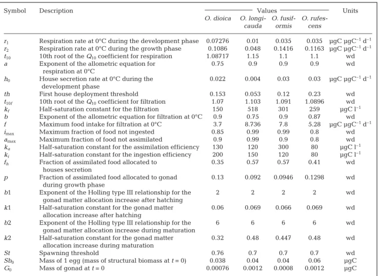
Model. The overall organisation and behaviour of our model was described by Lombard et al. (2009) for the appendicularian Oikopleura dioica (Appendix 1). This physiological model defines appendicularian growth as the difference between the intake of carbon (filtration, ingestion, assimilation) and the metabolic losses and expenses (faecal pellets, respiration, house secretion). The forcing variables are T (°C) and food concentration (µgC l–1). The simulated variables (car-bon units) are the appendicularian trunk and gonad mass, the mass of secreted houses, and the losses in discarded houses, faecal pellets and respiration. Here, we adapted the model for 3 additional appendicularian species, i.e. O. longicauda, O. fusiformis and O. rufe-scens (see below). The 4 modelled species are among the most abundant appendicularian species in the global ocean (Fenaux et al. 1998). The parameters used in the model are listed in Table 1.
The parameters controlling filtration and ingestion (f, t10f, b, kf, imax, ki) of Oikopleura longicauda,
O. fusiformis and O. rufescens were calculated directly from the data in Sato et al. (2005). For O. longicauda, the parameters controlling respiration (r2, t10 and a) were estimated from experimental results (Gorsky et al. 1984b) and from Lombard et al. (2005). Parameters corresponding to respiration and first house produc-tion during the larval stage were calibrated according to the length of the embryonic phase and the relative mass of a single house (Sato et al. 2003). The other pa-rameters were calibrated using least-square minimiza-tion (Nelder-Mead simplex method) between model outputs and experimental observations of growth that
included generation time (Fenaux & Gorsky 1983, Sato et al. 2003), and energy budget of house secretion (Sato et al. 2003). This algorithm made it possible to lo-cate the set of parameters that minimized the differ-ences between the model and the experimental data.
A specific carbon to chlorophyll a ratio (C:chl a) (Flynn et al. 1994) obtained with the haptophyte Iso-chrysis galbana was used for the experimental results (i.e. the experiments that involved the appendicularian species; Sato et al. 2003). All experimental data and in situ observations expressed in chl a concentrations were transformed into carbon units using the variable C:chl a conversion factor issue from the PISCES model (Aumont & Bopp 2006). This model implemented worldwide the phytoplankton growth model of Geider et al. (1997), and provided C:chl a ratios as a function of latitude, season, and depth, taking into account the influence of T, irradiance and nutrient availability. The variable C:chl a ratio provides a better representation of food availability than a constant ratio, but phyto-plankton does not represent the whole range of
parti-cles grazed by appendicularians at sea, which also include heterotrophic organisms (i.e. bacteria and microzooplankton) and small organic detritus. Even if appendicularian food in our model should take into account the types, size spectra and quality of potential food particles, the only data available in most cases are chl a concentrations. In such situations, we used chl a as a first order estimator of the available food.
In situ observations in the English Channel. In order
to validate model predictions (below) against seasonal successions of appendicularians, we used in situ obser-vations of appendicularians made by López-Urrutia et al. (2005) in the English Channel. Because our model is based on the physiology of organisms, it can only be applied when physiology is the main factor controlling appendicularian succession. In other words, it cannot be used when horizontal transport by currents controls the appendicularian assemblages. We then focussed our study on samples from the L4 site (off Plymouth, UK), which is the only location where a succession involving 3 of the 4 modelled species was observed. Table 1. Oikopleura spp. Model parameters: symbol, description, value and units for the 4 appendicularian species. wd:
dimensionless
Symbol Description Values Units
O. dioica O. longi- O. fusif- O.
rufes-cauda ormis cens
r1 Respiration rate at 0°C during the development phase 0.07276 0.01 0.035 0.035 µgC µgC–1d–1 r2 Respiration rate at 0°C during the growth phase 0.1086 0.048 0.1416 0.1163 µgC µgC–1d–1 t10 10th root of the Q10coefficient for respiration 1.08717 1.15 1.1 1.1 wd
a Exponent of the allometric equation for 0.75 0.9 0.9 0.9 wd
respiration at 0°C
h0 House secretion rate at 0°C during the 0.022 0.004 0.03 0.03 µgC µgC–1d–1
development phase
th First house deployment threshold 0.153 0.053 0.12 0.23 wd
t10f 10th root of the Q10coefficient for filtration 1.07 1.103 1.091 1.0896 wd
kf Half-saturation constant for the filtration 150 518 301 259 µgC l–1
b Exponent of the allometric equation for filtration at 0°C 0.9 0.75 0.9 0.87 wd
f Maximum food intake for filtration at 0°C 3.7 8.736 7.8 5.28 µgC µgC–1d–1
imax Maximum fraction of food not ingested 0.85 0.99 0.99 0.8 wd
amax Maximum fraction of food not assimilated 0.9 0.99 0.9 0.8 wd
ka Half-saturation constant for the assimilation efficiency 130 120 300 80 µgC l–1
ki Half-saturation constant for the ingestion efficiency 200 150 120 80 µgC l–1
fh Fraction of assimilated food allocated to 0.35 0.57 0.57 0.41 wd
houses secretion
p Fraction of assimilated food allocated to gonad 0.13 0.092 0.0946 0.1298 wd during growth phase
b1 Exponent of the Holling type III relationship for the 2 2 2 2 wd
gonad matter allocation increase after hatching
k1 Half-saturation constant for the gonad matter 0.06 0.069 0.066 0.069 wd allocation increase after hatching
b2 Exponent of the Holling type III relationship for the 6 6 6 6 wd
gonad matter allocation increase during maturation
k2 Half-saturation constant for the gonad matter 0.32 0.48 0.447 0.48 wd allocation increase during maturation
St Spawning threshold 0.76 0.7 0.7 0.7 wd
Sb0 Mass of 1 egg (mass of structural biomass at t = 0) 0.038 0.04 0.04 0.06 µgC
The organisms were collected weekly with 200 µm mesh plankton nets (vertical tows: 0 to 50 m) in 1999 and 2000. All appendicularian species were identified and enumerated.
In order to apply our model, we used the T and chl a observed weekly at the same location and during the same period as appendicularians. The data had been sampled weekly using a CTD (T °C) or a fluorimetric method on water sampled at 10 m (chl a). The potential food for appendicularians (µgC l–1) was estimated from the observed chl a using a seasonally variable C:chl a ratio at the corresponding depth and location (PISCES model; see ‘Model’).
In situ observations from satellite images. In order to
apply the model on a larger geographic scale, we used the mean seasonal values (2002 to 2005) of sea surface temperature (SST) and ocean colour derived chl a from the MODIS satellite (OceanColor Web, NASA, http:// oceancolor.gsfc.nasa.gov/). Because the ocean colour images do not include the sub-surface chl a maximum, we estimated the depth and concentration of this chl a maximum following the methodology developed by Morel & Berthon (1989) as modified by Uitz et al. (2006). The available food concentration (µgC l–1) was esti-mated for each season using the PISCES variable C:chl a ratio at the depth of the chl a maximum.
In situ observations in the North Atlantic. In situ
observations of appendicularians were made in the North Atlantic Ocean during the POMME (Programme Ocean Multidisciplinaire Meso Echelle) research crui-ses. The study area was located off the Iberian Penin-sula (39 to 45°N, 15 to 21°W). Sampling took place in winter 2001 (POMME 1), spring 2002 (POMME 2) and late summer 2002 (POMME 3). Each cruise consisted of 2 legs: Leg 1 was a spatial survey of the study zone, and Leg 2 focused on selected ‘long stations’ that were sampled during 48 h.
During Leg 2 of the POMME 3 cruise, the UVP model 4 (UVP4) (Gorsky et al. 2000b) was deployed at 4 stations, where it recorded large numbers of appen-dicularians. These were not represented in the oblique BIONESS zooplankton tows (0 to 700 m oblique tows; 500 µm mesh size), and were largely undersampled in the vertical WP2 tows (0 to 200 m vertical tows; 200 µm mesh size; V. Andersen & L. Mousseau, pers. comm.). The UVP recorded information on particles >100 µm, i.e. large marine snow and zooplankton. Abundances and size distributions of living and non-living objects were determined down to 1000 m depth. The UVP4 uses two 54 W Chadwick Helmuth stroboscopes syn-chronized with 2 video cameras. The beams are spread into a structured 8 cm thick slab by 2 mirrors. The par-ticles illuminated in volumes of 1.25 and 10.5 l are recorded simultaneously by the 2 cameras. Appendic-ularians were counted from the wide-angle camera,
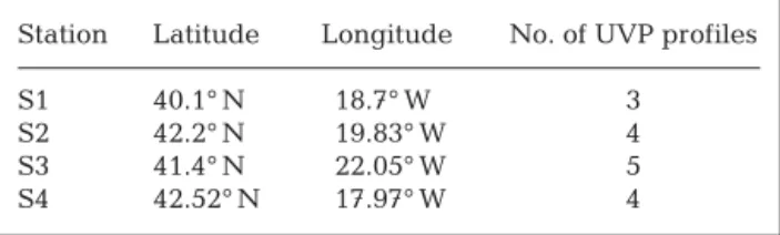
which surveys ~120 m3for a 0 to 1000 m cast. The short duration of the flashes (pulse duration = 30 µs) allows for a fast lowering speed (up to 1.5 m s–1) without dete-riorating image quality. The 0 to 1000 m water column was sampled with only minor overlapping between 2 successive images. The images are processed in situ during the recovery of the instrument. The total num-ber of profiles recorded at each station are given in Table 2. All profiles were examined by experts and appendicularians enumerated. For each station, the mean concentration of appendicularians were calcu-lated over 5 m depth bins.
Additional information was collected with a CTD SBE911 Rosette. Total particulate carbon (TPC) was estimated from bio-optical profiles (spectrophotometer ac-9 WETLabs®; Moore 1994) by converting the 555 nm beam attenuation into TPC using the conver-sion factor determined during the cruise, compared to water samples filtered through GF/F filters and analysed with a Robobrep Europa Scientific®analyzer (Merien 2003). TPC was used as food concentration in the model. This measurement is probably more repre-sentative of the food available to appendicularians than chl a, despite the fact that TPC includes large par-ticles that appendicularians cannot filter as well as detritic matter of low nutritional value.
From the in situ observations of abundance, we esti-mated the effect of filter-feeding appendicularians on the consumption of small particles (e.g. algae, bacte-ria), the production of large particles (discarded houses, faecal pellets), and the organic matter involved in respiration and growth. We proceeded in 2 steps: firstly, we identified the species having the highest growth rate based on environmental parameters (food concentration in carbon units, T °C), which we assumed to be the dominant appendicularian species; secondly, we used the model parameterized for that species for the whole life cycle of the appendicularian using the observed environmental conditions in order to esti-mate the mean daily rates of filtration, growth, respira-tion, and house and pellet production. We used these individual rates to calculate a resulting rate for the whole population observed at every depth bin at each sampling station.
Table 2. Geographical locations of stations during the POMME 3 Leg 2 cruise, and number of UVP profiles used for
appendicularian identification
Station Latitude Longitude No. of UVP profiles
S1 40.1° N 18.7° W 3
S2 42.2° N 19.83° W 4
S3 41.4° N 22.05° W 5
RESULTS AND DISCUSSION Model calibration
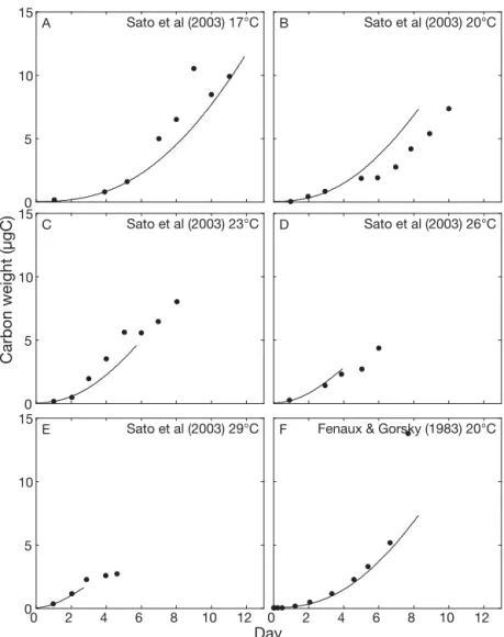
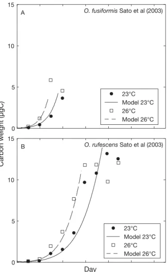
The results of model calibrations on the life cycles of Oikopleura longicauda, O. fusiformis and O. rufescens are presented in Figs. 1 & 2. The parameter values for each species resulting from the calibration are given in Table 1. Figs.1 & 2 show that a single model based on a small number of physiological observations (Sato et al. 2003, 2005), and calibrated with species specific sets of parameters is sufficient to simulate each of their life cycles.
Simulations are consistent with observations ob-tained for the species grown at different T (Figs. 1 & 2). Growth rates are correctly estimated until the begin-ning of reproduction (i.e. 1 or 2 d before the end of the experiment). The length of the life cycle is also
cor-rectly reproduced, even if the life span of O. longi-cauda and O. rufescens are underestimated at the highest T (Figs. 1 & 2). This small discrepancy may be due to over-simplified representation of the length of the spawning window in the model, which considers the properties of a single mean individual, whereas in the real population, individual variability exists due notably to the fact that the larger, ripe individuals released their gametes and died before the slowly growing individuals, which reproduce later (Sato et al. 2003). The early spawning of the largest individuals could explain the negligible growth of O. rufescens observed at the end of its life cycle (Fig. 2). However, this possible misrepresentation of the life span at high T has no effect on the estimates of growth rate, and only the estimates are used in the following applica-tions.
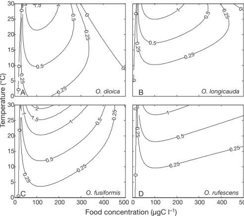
Growth rates and ecological niches Over a wide range of stable condi-tions of food and T, the model simulates similar trends of growth rates for the 4 species (i.e. including Oikopleura dioica; Lombard et al. 2009) (Fig. 3) with optimum values observed in mesotrophic conditions and for high
T (i.e. 100 to 150 µgC l–1, T > 25°C). Of
the 4 species, O. fusiformis shows the highest growth rate under these optimum conditions. Fig. 3 also indi-cates the environmental conditions that may support positive growth for the different species. Compared to O. dioica (Fig. 3A), the other 3 species (Fig. 3B,C,D) seem to have higher growth at high food concentrations. In addition, O. longicauda seems to be strongly growth limited at low T (Fig. 3B) and O. rufescens appears only little affected by high food concentra-tions (Fig. 3D).
The limits within which the growth is positive provide a first indication of the breadth of the fundamental niche according to Levins (1968), who defined the ecological niche as a measure of fit-ness in a multidimensional space. How-ever, definitions of the fundamental niche may be inappropriate for natural populations because when several spe-cies are present, their ecological niches are reduced by competitive exclusion and thus become realized niches
0 2 4 6 8 10 12
F Fenaux & Gorsky (1983) 20°C
0 2 4 6 8 10 12 0 5 10 15 Day E Sato et al (2003) 29°C 0 5 10 15 A Sato et al (2003) 17°C 0 5 10 15 Carbon weight (µgC) C Sato et al (2003) 23°C D Sato et al (2003) 26°C B Sato et al (2003) 20°C
Fig. 1. Oikopleura longicauda. Growth curves at different temperatures. Dots: experimental data from Sato et al. (2003) and Fenaux & Gorsky (1983). Lines:
(Hutchinson 1957). We obtained a simplified estima-tion of the realized niche breadth for each of the 4 spe-cies by comparing their growth rates, and thus deter-mined which species has the highest growth rate under a set of environmental conditions. This approach is implemented in Fig. 4 and is, as far as we know, the first estimation of the realized niches of appendicular-ian species related to their physiology and growth abil-ity as a function of T and food concentration.
Using this simplified representation of the realized niche of each species, we defined, with due considera-tion of the limitaconsidera-tions of the approach (Hutchinson 1961, Wilson 1990), the environmental conditions within which each species has the highest growth rate
and may thus theoretically dominate the assemblage. Fig. 4 shows that Oikopleura dioica does well in low-T (< 20°C) mesotrophic to eutrophic conditions, O. longi-cauda has higher growth rates than other species in oligotrophic conditions, O. fusiformis is dominant in warm (above 20°C) mesotrophic to eutrophic condi-tions, and O. rufescens shows the highest growth rate in highly eutrophic conditions.
The realized niches in Fig. 4 must be considered with caution, because mortality and predation are not rep-resented in the model. There are also other limitations to these ecological realized niches. Firstly, our study considers 4 appendicularian species only, i.e. it does not take into account other appendicularian species or other groups of organisms. Introduction of other appendicularians in the model, such as the typically cold water species Oikopleura vanhoeffeni, O. labra-dorensis and Fritilaria borealis, could reduce the breadth of the realized niche of O. dioica, O. longi-cauda and O. rufescens in cold waters. Similarly, intro-duction of organisms belonging to other groups such as salps, copepods and fishes, may significantly reduce the realized niche of appendicularians by competition and predation (Sommer et al. 2003, López-Urrutia et al. 2004, Stibor et al. 2004); hence, especially in the case of clearly limiting conditions (i.e. cold water or low food concentration) where appendicularian growth rates are low, the actual limits of the realized ecological niches could be somewhat different from those in Fig. 4. Secondly, the growth rates we estimated origi-nate from model simulations under constant food and T conditions, and may be different in fluctuating envi-ronments, e.g. in cases of rapid changes in T (e.g. wind events, currents) or food concentration (e.g. blooms). Given the high growth rates of all appendicularian species in mesotrophic to eutrophic conditions, the one present in the ecosystem under limiting conditions could rapidly respond to increasing food. Hence, it is possible that the composition of the appendicularian assemblage that dominates during a high-food event is influenced by the species response to food-limited con-ditions prior to the event. Thirdly, our model only takes into consideration T and food concentration, and does not consider other environmental conditions such as salinity. It is known that some appendicularian species can have different behaviour under different salinity conditions (Sato et al. 2001, López-Urrutia et al. 2005), but as the effects of salinity on physiological rates are poorly known, it was preferable to not include them in our model.
Despite these limitations, the realized niches of the 4 species in Fig. 4 are consistent with field observations. Indeed in the ocean, Oikopleura dioica is found in tem-perate waters, and O. longicauda, O. fusiformis and O. rufescens are common in warm waters (López-0 5 10 15 A O. fusiformis Sato et al (2003) 23°C Model 23°C 26°C Model 26°C 0 5 10 15 Day Carbon weight (µgC) B O. rufescens Sato et al (2003) 23°C Model 23°C 26°C Model 26°C
Fig. 2. Oikopleura fusiformis, O. rufescens. Growth of (A)
O. fusiformis and (B) O. rufescens at different temperature
(T ). Dots: experimental data from Sato et al. (2003). Lines: model simulations. At 23 and 26°C (O. rufescens) and 26°C (O. fusiformis), the last experimental points correspond to the end of reproduction period. As these organisms died after spawning, the population stopped increasing in size (plateau); these points were not used in the model calibration
Urrutia et al. 2005). Moreover, in warm oligotrophic systems, O. longicauda was observed to be dominant, whereas O. fusiformis occurred only in small numbers (Scheinberg et al. 2005). It follows that our approach can be used to determine the potentially dominant
appendicularian species based on the prevailing T and food concentra-tion observed at sea.
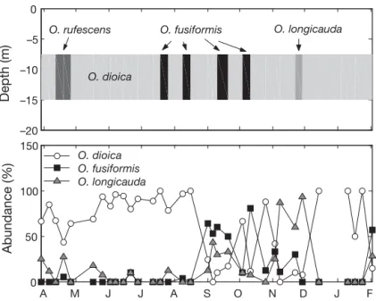
Model validation and application: seasonal species succession We validated our realized ecologi-cal niche approach by running the model with T and potential food observed in the English Channel during 1999–2000 (López-Urrutia et al. 2005). We compared the succes-sion of dominant species predicted by the model with the observed spe-cies composition at sea (Fig. 5). Our model applied to the above 4 appen-dicularian species predict that Oiko-pleura dioica would have the high-est growth rate nearly during the whole period and would then be the dominant species except in few time intervals. In April 1999, an intense bloom of phytoplankton was recor-ded during 3 wk (maximum concen-tration: 9.8 mg chl a m– 3), leading to the prediction of dominance by O. rufescens. From the end of July to October 1999, because of warmer conditions combined with higher food concentration, O. fusiformis was pre-dicted to be the dominant species in an alternation with O. dioica. In December 1999, low food conditions led the model to estimate that O. longicauda could be the dominant species. This predicted seasonal succes-sion is in good agreement with the available observa-tions (López-Urrutia et al. 2005, our Fig. 5). O. dioica was the dominant oikopleurid species nearly all the year. From September to October, with a ~6 wk delay compared to the first appearance predicted by the model, O. fusiformis appear to be the dominant species in an alternative way with O. dioica. Finally, O. longi-cauda was dominant from November to December 1999. However, the predicted dominance of O. rufe-scens during 3 wk in April was not observed during the survey.
One potential bias of our approach is that the amount of food available to appendicularians may have been underestimated as it was based only on chl a without including other potential living and non-living food particles. A second limitation is that chl a was only measured at one depth (10 m). Despite these limita-tions, the model outputs matched the observations quite well. This indicates that the physiological behav-iour of appendicularians as a function of T and food
0 100 200 300 400 500 0 0 0.25 0.25 0.25 0.5 1 D O. rufescens 0 100 200 300 400 500 0 5 10 15 20 25 30 Food concentration (µgC l–1) Temperatur e (°C) 0 0 0.25 0.25 0.25 0.5 0.5 1 1 1.5 2 C O. fusiformis 0 5 10 15 20 25 30 0 0 0 0 0 0.25 0.25 0.25 0.5 0.5 1 1 1.5 A O. dioica 0 0 0 0. 25 0.25 0.25 0.5 0.5 1 B O. longicauda
Fig. 3. Oikopleura spp. Daily growth rates (d–1) of (A) O. dioica, (B) O. longicau-da, (C) O. fusiformis and (D) O. rufescens as a function of temperature and food
concentration
Fig. 4. Oikopleura spp. Realized ecological niches of the 4 appendicularians obtained by comparing their respective growth rates as a function of temperature and food
concentration can explain the general pattern of the seasonal succession of appendicularian species.
Model application: ocean-wide biogeography of appendicularians
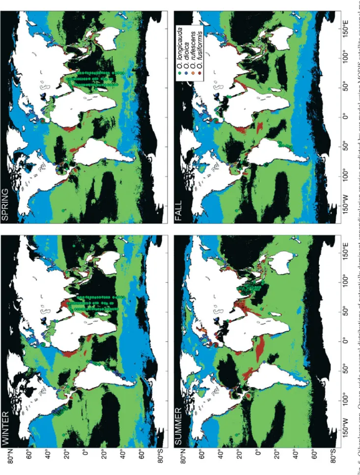
Using the global scale data of T and MODIS satellite derived chl a, we further used our model to predict the worldwide distributions of dominance (i.e. highest growth rate) among the 4 appendicularian species (Fig. 6). This result is, as far as we know, the first attempt to provide a seasonal description of appendic-ularians ocean-wide biogeography based on sea sur-face conditions.
In Fig. 6, Oikopleura dioica is generally dominant in temperate regions and in coastal ecosystems because of its success at T < 20°C and in meso-eutrophic condi-tions (Fig. 4). Our model results in temperate and sub-tropical conditions are consistent with the reported neritic preference of this species, but the model also suggest that O. dioica may also be dominant offshore between 30 and 60° latitude in the 2 hemispheres, with an even wider latitudinal distribution in the North. Because information on appendicularian species is, to our knowledge, missing in these regions, the hypothe-sis of dominance by O. dioica offshore needs to be tested by sampling. According to the model, O. dioica is also dominant in the coastal upwelling areas of Cali-fornia, Chile, Mauritania and Benguela. The
geogra-phic dominance of O. dioica is broadest in winter and spring. During summer, the domi-nance of O. dioica is restricted to a narrow zone along coastlines and is replaced offshore by O. longicauda. Species O. longicauda is especially successful in oligotrophic condi-tions (Fig. 4), and its widest zone of domi-nance is from equatorial to temperate regions (Fig. 6); it can grow and dominate the appen-dicularian assemblage in oligotrophic off-shore areas. In winter, this species is domi-nant in tropical oligotrophic offshore waters. During summer in the centre of the tropical offshore waters, the food concentration becomes so low that it no longer allows this species to grow, and as the offshore subtropi-cal and temperate zones become more oligo-trophic, O. longicauda replaces O. dioica and becomes dominant. Species O. fusiformis is typically successful in warm waters (> 20°C) and in meso- to eutrophic conditions (Fig. 4). As a consequence, it dominates the appendic-ularian assemblages in upwelling and coastal areas between 20°N and 20°S, and also domi-nates during summer in coastal temperate regions. Because it is mostly successful in highly eutrophic, warm conditions, O. rufescens dominates the appendicularian assemblage in a few coastal tropi-cal regions only. In tropitropi-cal offshore ecosystems, the available food does not seem to be sufficient to support the growth of any of the 4 species. These conclusions are limited by the fact that the amount of food calcu-lated by the model is based on in situ chl a concentra-tion, which may have underestimated the total avail-able food. This limitation does not likely cause large discrepancies in mesotrophic and eutrophic condi-tions, but it could lead to food underestimation in highly oligotrophic conditions where the ratio of phytoplankton carbon to total particulate organic car-bon is lower than in richer environments (Legendre & Michaud 1999, their Eqs. 11 & 12).
We compared our model predictions (Fig. 6) with the actual dominance of the 4 species at sea (Table 3, 517 field observations). The results of comparison are (1) model predictions matched 71% of the observa-tions, (2) the dominant species was incorrectly pre-dicted in only 16% of cases, and (3) in 13% of cases, the model predicted that none of the species could grow where Oikopleura longicauda was actually recorded. The observed differences between model predictions and observations, such as the prediction of dominance by O. longicauda instead of O. fusiformis in South European seas during summer and autumn, or the actual dominance of O. longicauda in the central Indian Ocean where the model predicted no appendic-–20 –15 –10 –5 0 Depth (m) O. fusiformis O. dioica O. longicauda O. rufescens A M J J A S O N D J F 0 50 100 150 Abundance (%) O. dioica O. fusiformis O. longicauda
Fig. 5. Oikopleura spp. Seasonal succession of appendicularians in the English Channel (upper panel) predicted by our model based on sea-sonal variations of temperature and food concentration, and observed dominant species at 0–50 m during 1999–2000 (López-Urrutia et al.
Fig. 6.
Oikopleura
spp.
Ocean-wide seasonal distributions of potentially dominant appendicularian species pr
edicted by our model using MODIS satell
ite seasonal mean
sea sur face temperatur e and chl a , compar ed to in situ data (dots) fr om the literatur e (T able 3). Blue: Oikopleura dioica . Gr een: O. longicauda . Br own: O. fusifor mis . Orange: O. r ufescens
ularian growth, are probably related to underestima-tion of real food concentraunderestima-tion when taking phyto-plankton as the only potential food. Despite this limita-tion, the model generally predicted correctly the most probable dominant appendicularian species in various offshore and inshore systems, from T and food concen-tration. Our model provides an approach for including appendicularians in ecological-biogeochemical mod-els that consider plankton functional types.
Model application: role of appendicularians in downward carbon flux
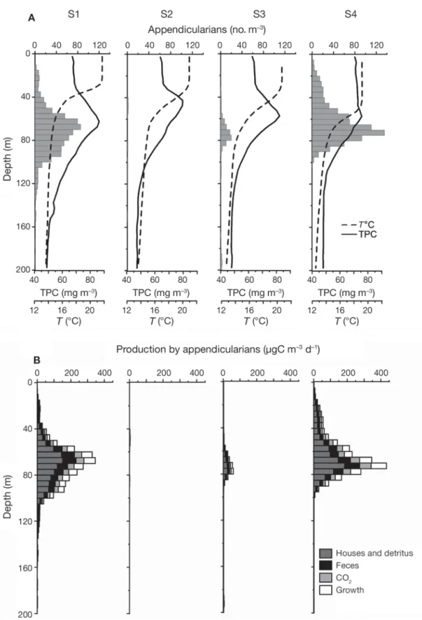
During the POMME 3-Leg 2 cruise in the North Atlantic, large numbers of appendicularians were ob-served with the UVP at Sites 1 (S1) and 4 (S4), with maximum concentrations of 85 and 135 ind. m– 3at 65 and 70 m, respectively (Fig. 7). In contrast, few appen-dicularians were observed at Sites 2 (S2) and 3 (S3),
where the maximum abundance were 2 and 11 ind. m– 3, respectively. Moreover, the UVP continuous re-cords at depth showed that appendicularians were mostly concentrated near the maximum TPC concen-tration, below the thermocline. The observed numbers of appendicularians were low compared to some coastal regions were they can exceed 10 000 ind. m– 3 (Taguchi 1982, Ashjian et al. 1997, Hopcroft & Roff 1998, Fernández & Acuña 2003, Maar et al. 2004, Scheinberg et al. 2005). This is consistent with the fact that appendicularians generally bloom in mesotrophic or eutrophic coastal conditions, whereas the POMME 3 observations were made in offshore oligotrophic con-ditions.
The data on the vertical distribution of appendicular-ians abundance and on T and TPC were used to deter-mine the species with the highest potential growth rate. Our model predicted that Oikopleura dioica was the best candidate for the whole sampling area (except for the upper 25 m at S1 where O. fusiformis was pre-Table 3. Observations of appendicularian species composition in the World Ocean: location, sampling season (Sp: spring; Su:
summer; F: fall; W: winter; All: all seasons; An. Mean: annual mean), number of observations (n) and source
Location Sampling n Source
season Atlantic Ocean
Norwegian fjord All 4 López-Urrutia et al. (2005) Norwegian fjord All 4 López-Urrutia et al. (2005) Norwegian fjord All 4 López-Urrutia et al. (2005) Swedish fjord Sp & F 2 Vargas et al. (2002) Skagerrak Su & F 2 Maar et al. (2004) North Sea An. Mean 4 Le Fevre-Lehoerff et a (1995)
North Sea All 4 Greve (2005)
English Channel All 4 Acuña et al. (1995) English Channel All 4 López-Urrutia et al. (2005) Cantabrian Sea All 4 Acuña & Anadon (1992) Cantabrian Sea Su 36 Acuña (1994) Cantabrian Sea All 16 López-Urrutia et al. (2003) Cantabrian Sea All 12 López-Urrutia et al. (2005) South Carolina All 4 Costello & Stancyk (1983) Mississipi plume Sp 1 Dagg et al. (1996)
Florida All 4 Hopkins (1977)
Jamaica All 4 Hopcroft & Roff (1998) Caribbean Sea Sp & F 2 Osorio (2003) Northeastern W & Su 2 Silva et al. (2003) Brazil
Brazil An. Mean 4 Valentin et al. (1987) S America coast F 45 Fenaux (1967) Argentina W 5 Capitanio & Esnal (1998) S-W Atlantic Ocean F 12 Esnal & Castro (1977) Mediterranean Sea
Adriatic Sea All 4 Fenaux (1972a) Adriatic Sea Sp 1 Skaramuca (1977) Venice All 4 Brunetti et al. (1990)
Ligurian Sea All 4 Fenaux (1961)
Ligurian Sea All 4 López-Urrutia et al. (2005)
Location Sampling n Source
season Pacific Ocean
Orcas Island (WA) Sp 1 Hansen et al. (1996) California W 1 Landry et al. (1994) California W 1 Passow et al. (2001) California coast W 83 Fenaux & Dallot (1980) Inland Sea of Japan All 4 Uye & Ichino (1995)
Central Japan All 4 Itoh (1990)
Southern Japan Sea All 4 Tomita et al. (2003) Tokyo Bay All 4 Nomura & Murano (1992)
Korea All 4 Lee et al. (2001)
South China Sea W 1 Yang & Wang (1988) Eniwetok (Pacific) W 1 Gerber & Marshall (1974) Hawaii W & Sp 2 Scheinberg et al. (2005)
Hawaii An. Mean 4 Tagushi (1982)
Peru F 12 Fenaux (1968)
Northern Chile Su & Sp 2 Vargas & González (2004) Indian Ocean
Bay of Bengal Su 89 Fenaux (1969a)
Bay of Bengal Sp 1 Madhupratap
et al. (1980) Bay of Bengal Su 18 Sreekumaran Nair et al.
(1981) Indian Ocean W-Sp 67 Fenaux (1972b)
Madagascar All 4 Fenaux (1969b)
Seychelles Su 1 Fenaux (1980)
Black Sea An. Mean 4 Shiganova (2005) Red Sea
Gulf of Aqaba Su 1 Vaissiere & Seguin (1984) Gulf of Elat All 4 Fenaux (1979)
Fig. 7. Oikopleura spp. Vertical distributions of observed and modelled variables at 4 sampling sites during the POMME 3 Leg 2 cruise in the North Atlantic in 2001. (A) Observations: appendicularians recorded with the UVP (grey bars), total particulate car-bon estimated from bio-optical profiles (TPC, solid lines) and temperature (T, dashed lines). (B) Modelled daily production of ap-pendicularian detritus (faecal pellets and discarded houses with food particles trapped inside), body mass and CO2(respiration).
dicted to be the dominant species). Consequently, we hypothesized that O. dioica was the main appendicu-larian species in the POMME area in late summer 2001. This output of the model was confirmed by direct identification of appendicularian houses on the UVP profiles, and from WP2 net samples where most appen-dicularians were O. dioica. On the basis of appendicu-larian abundances and environmental conditions, we simulated the whole life cycle of O. dioica in order to estimate their daily effect on the consumption and aggregation of particulate matter and the fluxes of bio-genic carbon (Fig. 7). Because appendicularians are present in largest numbers below the thermocline, their impact on carbon fluxes should also be greatest there. Appendicularians in the POMME area had a rel-atively small effect on TPC consumption (sum of respi-ration, growth, faecal palettes and discarded houses productions, Fig. 7), i.e. only 0.6% of the total stock of TPC was grazed daily by appendicularians at the sta-tion and depth were their concentrasta-tion was highest (S4, 70 m). The TPC consumed was used with low effi-ciency by appendicularians for growth, i.e. at the depth of maximum appendicularian concentration, 65% of the TPC grazed was lost in the form of large aggre-gates (i.e. discarded houses and faecal pellets), 14% was remineralised through respiration and only 21% was used for growth. As the aggregates are generally produced by appendicularians mostly under the ther-mocline and have sinking rates of 50 to 120 m d–1 (Gorsky et al. 1984a, Alldredge 2005, Dagg & Brown 2005), they can reach a depth of 200 m within 1 to 3 d in low turbulence conditions. Hence, we could com-pare the production of aggregates by appendicularians with the total flux of particulate organic carbon (POC) from sediment traps moored at 200 m (Fig. 8). Fig. 8 shows that the amount of sinking matter sampled at 200 m did not correspond to the production of aggre-gates by appendicularians, i.e. the latter was lower than the sediment trap flux at S2 and S3, and higher at S1 and S4. The low production at S2 and S3 reflects the low concentrations of appendicularians. The situation at S1 and S4 requires further discussion.
Our study is not the first to predict a production of particulate matter by appendicularians that exceeds the observed total sinking flux, e.g. in the literature, calculated production of discarded houses represented only 12 to 83% of the total POC flux in sediment traps at depths < 200 m (Alldredge 2005), and the flux of fae-cal pellets did exceed the total POC flux at 25 and ~300 m depths (Dagg & Brown 2005, Deibel et al. 2005). The difference between simulated aggregate production and the observed flux in traps may reflect the relatively low efficiency of sediment traps, as observed during the POMME cruise for traps at 400 m (19 to 53% efficiency measured using thorium-230
iso-tope; Guieu et al. 2005). Indeed, discarded houses are sticky and may potentially have a different trapping efficiency compared to other material (faecal pellets). In addition, visual determination of particles collected in the traps showed that appendicularian detritus made up only a small fraction of the total. Hence, the difference between our model estimates of particulate matter produced by appendicularians and the flux of matter in sediment traps may also be due to rapid degradation or consumption of appendicularian aggre-gates above the depths of traps. There is evidence from other studies for these 2 effects, as discussed next.
Observations in a Swedish fjord showed that in sed-iment traps located at different depths, 70% of the discarded houses observed at 10 m disappeared between 10 and 30 m (Vargas et al. 2002). The POMME 3 cruise was undertaken at the end of the summer oligotrophic phase, when phytoplankton were largely dominated by pico- and nanophyto-plankton (Claustre et al. 2005) and appendicularian faecal pellets would mainly contain this type of plank-ton. Hansen et al. (1996a) showed that the faecal pel-lets of Acartia tonsa eating a nanoflagellate algal diet were more rapidly degraded by bacteria than those from a diatom diet, and lost more than 50% of their volume in only 9 h. In the case of thaliacean faecal pellets (in situ sampling), a 50% decrease in carbon Fig. 8. Oikopleura spp. Comparison of the integrated produc-tion of detritus by appendicularians (faecal pellets and dis-carded houses with food particles trapped inside) estimated from our model with the observed particulate organic carbon
content was observed within 30 h due to bacterial activity (Pomeroy et al. 1984). Hence, during the tran-sit down to 200 m, a large fraction of the appendicu-larian faecal pellets could have been degraded by bacteria. The same might have applied to discarded houses, but their degradation rate is unknown and may be enhanced by the microbial community, including ciliates, present in the food concentrating filters (Davoll & Silver 1986, Hansen et al. 1996b).
In addition to degradation, the aggregates, including freshly filtered particles in the houses and only par-tially digested organic matter in the faecal pellets, can be grazed upon by a large number of zooplankton spe-cies during the oligotrophic period. For example, cyclopoid copepods belonging to the genus Oithona are known to be coprophagous (Gonzáles & Smetacek 1994), and coprorhexy has been observed for several calanoid copepods (Lampitt et al. 1990). In addition, copepods of the genera Oncaea and Calanus and euphausiids can all feed intensively on discarded houses (Alldredge 1972, 1976, Dagg 1993, Ohtsuka et al. 1993, Dilling et al. 1998). All these taxonomic groups were present during the POMME cruise (V. Andersen & L. Mousseau, pers. comm.) Hence, the aggregates produced by appendicularians could have been partly recycled by the food web instead of being exported to the deeper waters.
CONCLUSIONS
From the conditions of T and food concentration existing in different oceanic environments, a physio-logical model was used to estimate the realized niches of 4 appendicularian species, predict their seasonal succession, provide a seasonal ocean-wide biogeogra-phy of their distribution, and compare their predicted production of aggregates with the flux of POC within sediment traps. It was shown that this model can pro-vide first-order estimates of the most probably present appendicularian species. The next stage of model development would be to include the biology of popu-lations, which would take into account niche overlaps of the different species, simulating the effect of a fluctuating environment and the abundance of the different appendicularian species. However, most pop-ulation biology processes (i.e. predation on appendicu-larians, mortality and fecundity) are still poorly docu-mented at sea and thus need focussed research. Another improvement of the model would be the inclu-sion of key processes of degradation/consumption of the particles produced by appendicularians in order to estimate particle changes during their downward tran-sit. However, most of these processes are not presently known under field conditions.
Acknowledgements. We thank A. Lopez for providing the
data from the English Channel, L. Bopp for providing outputs of the PISCES model, and P. Nival, D. Deibel, J. L. Acuña, C. Poggiale, F. Carlotti, L. Stemmann and E. Urban for con-structive discussions. We thank the 4 anonymous reviewers for their constructive comments that allowed us to improve the manuscript. We also thank the EC FP6 SESAME project Contract No. GOCE-2006-036949, the French ZOOPNEC program, the MARBEF, EUR-OCEANS European Networks of Excellence and the Marie Curie Intra-European Fellowship No. 221696 for financial support.
LITERATURE CITED
Acuña JL (1994) Summer vertical distribution of appendicu-larians in the Central Cantabrian Sea (Bay of Biscay). J Mar Biol Assoc UK 74:585–601
Acuña JL, Anadon R (1992) Appendicularian assemblages in a shelf area and their relationship with temperature. J Plankton Res 14:1233–1250
Acuña JL, Bedo AW, Harris RP, Anadon R (1995) The seasonal succession of appendicularians (Tunicata: Appendicu-laria) off Plymouth. J Mar Biol Assoc UK 75:755–758 Alldredge AL (1972) Abandoned larvacean houses: a unique
food source in the pelagic environment. Science 177: 885–887
Alldredge AL (1976) Discarded appendicularian houses as sources of food, surface habitats, and particulate organic mater in planktonic environments. Limnol Oceanogr 21: 14–23
Alldredge AL (2005) The contribution of discarded appendic-ularian houses to the flux of particulate organic carbon from oceanic surface waters. In: Gorsky G, Youngbluth MJ, Deibel D (eds) Response of marine ecosystems to global change: ecological impact of appendicularians. GB Scientific Publisher, Paris, p 309–326
Ashjian C, Smith S, Bignami F, Hopkins T, Lane P (1997) Dis-tribution of zooplankton in the Northeast Water Polynya during summer 1992. J Mar Syst 10:279–298
Aumont O, Bopp L (2006) Globalizing results from ocean in situ iron fertilization studies. Global Biogeochem Cycles 20, GB2017, doi:10.1029/2005GB002591
Benfield MC, Davis CS, Wiebe PH, Gallager SM, Lough RG, Copley NJ (1996) Video plankton recorder estimates of copepod, pteropod and larvacean distributions from a stratified region of Georges Bank with comparative mea-surements from a MOCNESS sampler. Deep-Sea Res II 43: 1925–1945
Brunetti R, Baiocchi L, Bressan M (1990) Seasonal distribution of Oikopleura (Larvacea) in the lagoon of Venice. Boll Zool 57:89–94
Capitanio FL, Esnal GB (1998) Vertical distribution of ma-turity stages of Oikopleura dioica (Tunicata, Appen-dicularia) in the frontal system off Valdes Peninsula, Argentina. Bull Mar Sci 63:531–539
Claustre H, Babin M, Merien D, Ras J and others (2005) Toward a taxon-specific parameterization of bio-optical models of primary production: a case study in the North Atlantic. J Geophys Res 110, C07S12, doi:10.1029/ 2004JC002634
Costello J, Stancyk SE (1983) Tidal influence upon appendic-ularian abundance in North Inlet estuary, South Carolina. J Plankton Res 5:263–277
Dagg MJ (1993) Sinking particles as a possible source of nutrition for the copepod Neocalanus cristatus in the sub-arctic Pacific Ocean. Deep-Sea Res I 40:1431–1445
➤
➤
➤
➤
➤
➤
➤
➤
➤
Dagg MJ, Brown SL (2005) The potential contribution of fecal pellets from the larvacean Oikopleura dioica to vertical flux of carbon in a river dominated coastal margin. In: Gorsky G, Youngbluth MJ, Deibel D (eds) Response of marine ecosys-tems to global change: ecological impact of appendiculari-ans. GB Scientific Publisher, Paris, p 293–308
Dagg MJ, Green EP, McKee BA, Ortner PB (1996) Biological removal of fine-grained lithogenic particles from a large river plume. J Mar Res 54:149–160
Davis CS, Gallager SM, Berman MS, Haury LR, Strickler JR (1992) The video plankton recorder (VPR): design and ini-tial results. Arch Hydrobiol: Ergeb Limnol 36:67–81 Davoll PJ, Silver MW (1986) Marine snow aggregates: life
history sequence and microbial community of abandoned larvacean houses from Monterey Bay, California. Mar Ecol Prog Ser 33:111–120
Deibel D, Saunders PA, Acuña JL, Bochdansky AB, Shiga N, Rivkin RB (2005) The role of appendicularian tunicates in the biogenic carbon cycles of three Arctic polynyas. In: Gorsky G, Youngbluth MJ, Deibel D (eds) Response of marine ecosystems to global change: ecological impact of appendicularians. GB Scientific Publisher, Paris, p 327–356 Dennett MR, Caron DA, Michaels AF, Gallager SM, Davis CS (2002) Video plankton recorder reveals high abundances of colonial Radiolaria in surface waters of the central North Pacific. J Plankton Res 24:797–805
Dilling L, Wilson J, Steinberg D, Alldredge A (1998) Feeding by the euphausiid Euphausia pacifica and the copepod
Calanus pacificus on marine snow. Mar Ecol Prog Ser
170:189–201
Esnal GB, Castro RJ (1977) Distributional and biometrical study of appendicularians from the west South Atlantic Ocean. Hydrobiologia 56:241–246
Fenaux R (1961) Existence d’un ordre cyclique d’abondance relative maximale chez les Appendiculaires de surface (Tuniciers pélagiques). CR Hebd Seances Acad Sci Paris 253:2271–2273
Fenaux R (1967) Campagne de la Calypso au large des cotes Atlantiques de l’Amérique du Sud (1961–1962). Première partie. 5. Appendiculaires. Ann Inst Oceanogr 45:33–46 Fenaux R (1968) Algunas apendicularias de la costa Peruana.
Bol Inst Mar Peru 9:536–552
Fenaux R (1969a) Les appendiculaires du golfe du Bengale. Mar Biol 2:252–263
Fenaux R (1969b) Les appendiculaires de Madagascar (région de Nosy-Bé). Variations saisonnières. Cah ORSTOM Ser Oceanogr 7:29–37
Fenaux R (1972a) Variations saisonnières des appendiculaires de la region nord Adriatique. Mar Biol 16:310–319 Fenaux R (1972b) Les appendiculaires de la partie centrale de
l’océan Indien. J Mar Biol Assoc India 14:496–511 Fenaux R (1976) Cycle vital d’un appendiculaire Oikopleura
dioica Fol, 1872 description et chronologie. Ann Inst
Oceanogr 52:89–101
Fenaux R (1979) Preliminary data on ecology of appendicular-ians in Gulf of Elat. Isr J Zool 28:177–192
Fenaux R (1980) Les appendiculaires des Séchelles. Composi-tion de la populaComposi-tion. Etudes biométriques des espèces principales. Rev Zool Afr 94:795–806
Fenaux R (1986) Influence de la maille du fillet sur l’estima-tion des populal’estima-tions d’appendiculaires in situ. Rapp PV Reun Comm Int Explor Sci Mer Mediterr 30:203–204 Fenaux R, Dallot S (1980) Répartition des appendiculaires au
large des côtes de Californie. J Plankton Res 2:145–167 Fenaux R, Gorsky G (1983) Cycle vital et croissance de
l’ap-pendiculaire Oikopleura longicauda (Vogt), 1854. Ann Inst Oceanogr 59:107–116
Fenaux R, Palazzoli I (1979) Estimation in situ d’une popula-tion d’Oikopleura longicauda (Appendicularia) à l’aide de deux filets de maille différente. Mar Biol 55:197–200 Fenaux R, Bone Q, Deibel D (1998) Appendicularian
dis-tribution and zoogeography. In: Bone Q (ed) The biology of pelagic tunicates. Oxford University Press, Oxford, p 251–264
Fernández D, Acuña JL (2003) Enhancement of marine phyto-plankton blooms by appendicularian grazers. Limnol Oceanogr 48:587–593
Fernández D, López-Urrutia A, Fernández A, Acuña JL, Har-ris R (2004) Retention efficiency of 0.2 to 6 µm particles by the appendicularians Oikopleura dioica and Fritillaria
borealis. Mar Ecol Prog Ser 266:89–101
Flood PR (2005) Toward a photographic atlas on special taxo-nomic characters of oikopleurid Appendicularian (Tuni-cata). In: Gorsky G, Youngbluth MJ, Deibel D (eds) Response of marine ecosystems to global change: ecologi-cal impact of appendicularians. GB Scientific Publisher, Paris, p 59–85
Flynn KJ, Davidson K, Leftley JW (1994) Carbon–nitrogen relations at whole-cell and free-amino-acid levels during batch growth of Isochrysis galbana (Prymnesiophyceae) under conditions of alternating light and dark. Mar Biol 118:229–237
Gallienne CP, Robins DB (2001) Is Oithona the most important copepod in the world’s oceans? J Plankton Res 23: 1421–1432
Geider RJ, MacIntyre HL, Kana TM (1997) Dynamic model of phytoplankton growth and acclimation: responses of the balanced growth rate and the chlorophyll a:carbon ratio to light, nutrient-limitation and temperature. Mar Ecol Prog Ser 148:187–200
Gerber RP, Marshall N (1974) Ingestion of detritus by the lagoon pelagic community at Eniwetok Atoll. Limnol Oceanogr 19:815–824
González HE, Smetacek V (1994) The possible role of the cyclopoid copepod Oithona in retarding vertical flux of zooplankton faecal material. Mar Ecol Prog Ser 113: 233–246
Gorsky G, Fenaux R (1998) The role of Appendicularia in marine food webs. In: Bone Q (ed) The Biology of Pelagic Tunicates. Oxford University Press, Oxford, p 161–169
Gorsky G, Fisher NS, Fowler SW (1984a) Biogenic debris from the pelagic tunicate, Oikopleura dioica, and its role in the vertical transfer of a transuranium element. Estuar Coast Shelf Sci 18:13–23
Gorsky G, Palazzoli I, Fenaux R (1984b) Premières données sur la respiration des appendiculaires (tuniciers pélag-iques). CR Hebd Seances Acad Sci 298:531–534
Gorsky G, Aldorf C, Kage M, Picheral M, Garcia Y, Favole J (1992) Vertical distribution of suspended aggregates determined by a new underwater video profiler. Ann Inst Oceanogr 68:275–280
Gorsky G, Flood PR, Youngbluth M, Picheral M, Grisoni JM (2000a) Zooplankton distribution in four western Norwe-gian fjords. Estuar Coast Shelf Sci 50:129–135
Gorsky G, Picheral M, Stemmann L (2000b) Use of the Under-water Video Profiler for the study of aggregate dynamics in the North Mediterranean. Estuar Coast Shelf Sci 50:121–128
Greve W (2005) Biometeorology of North Sea appendiculari-ans. In: Gorsky G, Youngbluth MJ, Deibel D (eds) Res-ponse of marine ecosystems to global change: ecological impact of appendicularians. GB Scientific Publisher, Paris, p 277–290
➤
➤
➤
➤
➤
➤
➤➤
➤
➤
➤➤
➤
➤
➤
➤
➤
Guieu C, Roy-Barman M, Leblond N, Jeandel C and others (2005) Vertical particle flux in the northeast Atlantic Ocean (POMME experiment). J Geophys Res 110, C07S18, doi:10.1029/2004JC002672
Halliday NC, Coombs SH, Smith C (2001) A comparison of LHPR and OPC data from vertical distribution sampling of zooplankton in a Norwegian fjord. Sarsia 86:87–99 Hansen B, Fotel FL, Jensen NJ, Madsen SD (1996a) Bacteria
associated with a marine planktonic copepod in culture. II. Degradation of fecal pellets produced on a diatom, a nanoflagellate or a dinoflagellate diet. J Plankton Res 18: 275–288
Hansen JLS, Kiørboe T, Alldredge AL (1996b) Marine snow derived from abandoned larvacean houses: sinking rates, particle content and mechanisms of aggregate formation. Mar Ecol Prog Ser 141:205–215
Hopcroft RR, Roff JC (1995) Zooplankton growth rates: extra-ordinary production by the larvacean Oikopleura dioica in tropical waters. J Plankton Res 17:205–220
Hopcroft RR, Roff JC (1998) Production of tropical larvaceans in Kingston Harbour, Jamaica: Are we ignoring an impor-tant secondary producer? J Plankton Res 20:557–569 Hopcroft RR, Roff JC, Chavez F (2001) Size paradigms in
copepod communities: a re-examination. Hydrobiologia 453:133–141
Hopkins TL (1977) Zooplankton distribution in surface waters of Tampa Bay, Florida. Bull Mar Sci 27:467–478
Hutchinson GE (1957) Concluding remarks. Cold Spring Harb Symp Quant Biol 22:415–427
Hutchinson GE (1961) The paradox of the plankton. Am Nat 95:137–145
Itoh H (1990) Seasonal variation of appendicularian fauna off Miho Peninsula, Suruga Bay, central Japan. Bull Plankton Soc Japan 36:111–119
Lampitt RS, Noji T, von Bodungen B (1990) What happens to zooplankton faecal pellets? Implication for material flux. Mar Biol 104:15–23
Landry MR, Peterson WK, Fagerness VL (1994) Mesozoo-plankton grazing in the Southern California Bight. I. Pop-ulation abundances and gut pigment contents. Mar Ecol Prog Ser 115:55–71
Le Fevre-Lehoerff G, Ibanez F, Poniz P, Fromentin JM (1995) Hydroclimatic relationships with planktonic time series from 1975 to 1992 in the North Sea off Gravelines, France. Mar Ecol Prog Ser 129:269–281
Lee JH, Chae J, Kim WR, Jung SW, Kim JM (2001) Seasonal variation of phytoplankton and zooplankton communities in the coastal waters off Tongyeong in Korea. Ocean Polar Res 23:245–253
Legendre L, Michaud J (1999) Chlorophyll a to estimate the particulate organic carbon available as food to large zoo-plankton in the euphotic zone of oceans. J Plankton Res 21:2067–2083
Levins R (1968) Evolution in changing environments: some theoretical explorations. Princeton University Press, Princeton, NJ
Lombard F, Sciandra A, Gorsky G (2005) Influence of body mass, food concentration, temperature and filtering activ-ity on the oxygen uptake of the appendicularian
Oiko-pleura dioica. Mar Ecol Prog Ser 301:149–158
Lombard F, Sciandra A, Gorsky G (2009) Appendicularians ecophysiology. II. Reproducing clearance, growth, respi-ration and particles production of the appendicularian
Oikopleura dioica by modeling its ecophysiology. J Mar
Sys 78:617–629
López-Urrutia A, Acuña JL (1999) Gut throughput dynamics in the appendicularian Oikopleura dioica. Mar Ecol Prog
Ser 191:195–205 (Erratum in Mar Ecol Prog Ser 193:310, 2000)
López-Urrutia A, Irigoien X, Acuña JL, Harris R (2003) In situ feeding physiology and grazing impact of the appendicu-larian community in temperate waters. Mar Ecol Prog Ser 252:125–141
López-Urrutia A, Harris RP, Smith T (2004) Predation by calanoid copepods on the appendicularian Oikopleura
dioica. Limnol Oceanogr 49:303–307
López-Urrutia A, Harris RP, Acuña JL, Båmstedt U and others (2005) A comparison of appendicularian seasonal cycles in four distinct European coastal environments. In: Gorsky G, Youngbluth MJ, Deibel D (eds) Response of marine ecosystems to global change: ecological impact of appen-dicularians. GB Scientific Publisher, Paris, p 255–276 Maar M, Nielsen TG, Gooding S, Tonnesson K and others (2004)
Trophodynamic function of copepods, appendicularians and protozooplankton in the late summer zooplankton community in the Skagerrak. Mar Biol 144: 917–934 Madhupratap M, Devassy VP, Sreekumaran Nair SR, Rao TSS
(1980) Swarming of pelagic tunicates associated with phytoplankton bloom in the Bay of Bengal. Indian J Mar Sci 9:69–71
Merien D (2003) Variabilité biooptique à différentes échelles spatiales et temporelles dans l’Atlantique nord-est: inter-prétations biogéochimiques. PhD thesis, Université Pierre et Marie Curie, Paris
Moore C (1994) In-situ, biochemical, oceanic, optical meters. Sea Technol 35:10–16
Morel A, Berthon JF (1989) Surface pigments, algal biomass profiles, and potential production of the euphotic layer: relationships reinvestigated in view of remote-sensing applications. Limnol Oceanogr 34:1545–1562
Nomura H, Murano M (1992) Seasonal variation of meso- and macrozooplankton in Tokyo Bay, central Japan. Mer (Paris) 30:49–56
Norrbin MF, Davis CS, Gallager SM (1996) Differences in fine-scale structure and composition of zooplankton between mixed and stratified regions of Georges Bank. Deep-Sea Res II 43:1905–1924
Ohtsuka S, Kubo N, Okada M, Gushima K (1993) Attachment and feeding of pelagic copepods on larvacean houses. J Oceanogr 49:115–120
Osorio IAC (2003) Appendicularians (Tunicata) of Banco Chinchorro, Caribbean Sea. Bull Mar Sci 73:133–140 Passow U, Shipe RF, Murray A, Pak DK, Brzezinski MA,
All-dredge AL (2001) The origin of transparent exopolymer particles (TEP) and their role in the sedimentation of par-ticulate matter. Cont Shelf Res 21:327–346
Pomeroy LR, Hanson RB, McGillivary PA, Sherr BF, Kirchman D, Deibel D (1984) Microbiology and chemistry of fecal products of pelagic tunicates: rates and fates. Bull Mar Sci 35:426–439
Purcell JE, Sturdevant MV, Galt CP (2005) A review of appendicularians as prey of invertebrate and fish preda-tors. In: Gorsky G, Youngbluth MJ, Deibel D (eds) Response of marine ecosystems to global change: ecologi-cal impact of appendicularians. GB Scientific Publisher, Paris, p 359–435
Remsen A, Hopkins TL, Samson S (2004) What you see is not what you catch: a comparison of concurrently collected net, optical plankton counter, and shadowed image parti-cle profiling evaluation recorder data from the northeast Gulf of Mexico. Deep-Sea Res I 51:129–151
Robison BH, Reisenbichler KR, Sherlock RE (2005) Giant lar-vacean houses: rapid carbon transport to the deep sea floor. Science 308:1609–1611
➤
➤
➤
➤
➤
➤
➤
➤
➤
➤
➤
➤
➤➤
➤
➤
➤
➤
➤
➤
➤
➤
Samson S, Hopkins T, Remsen A, Langebrake L, Sutton T, Patten J (2001) A system for high resolution zooplankton imaging. IEEE J Oceanic Eng 26:671–676
Sato R, Tanaka Y, Ishimaru T (2001) House production by
Oikopleura dioica (Tunicata, Appendicularia) under
labo-ratory conditions. J Plankton Res 23:415–423
Sato R, Tanaka Y, Ishimaru T (2003) Species-specific house productivity of appendicularians. Mar Ecol Prog Ser 259: 163–172
Sato R, Tanaka Y, Ishimaru T (2005) Clearance and ingestion rates of three appendicularian species, Oikopleura
longi-cauda, O. rufescens and O. fusiformis. In: Gorsky G,
Youngbluth MJ, Deibel D (eds) Response of marine ecosystems to global change: ecological impact of appen-dicularians. GB Scientific Publisher, Paris, p 189–206 Scheinberg RD, Landry MR, Calbet A (2005) Grazing of two
common appendicularians on the natural prey assem-blage of a tropical coastal ecosystem. Mar Ecol Prog Ser 294:201–212
Shiganova T (2005) Changes in appendicularian Oikopleura
dioica abundance caused by invasion of alien ctenophores
in the Black Sea. J Mar Biol Assoc UK 85:477–494 Silva TA, Neumann-Leitão S, Schwamborn R, Gusmão LMO,
Nascimento-Vieira DA (2003) Diel and seasonal changes in the macrozooplankton community of a tropical estuary in Northeastern Brazil. Rev Bras Zool 20:439–446 Skaramuca B (1977) Distribution of Oikopleura longicauda
and Oikopleura fusiformis (Appendicularia) in the Adri-atic Sea. Rapp PV Réun Comm Int Expl Sci Mer Méditerr Monaco 24:147–148
Sommer F, Hansen T, Feuchtmayr H, Santer B, Tokle N, Sommer U (2003) Do calanoid copepods suppress appen-dicularians in the coastal ocean? J Plankton Res 25: 869–871
Sreekumaran Nair SR, Nair VR, Achuthankutty CT, Mad-hupratap M (1981) Zooplankton composition and diversity in western Bay of Bengal. J Plankton Res 3:493–508 Stemmann L, Youngbluth M, Robert K, Hosia A and others
(2008) Global zoogeography of fragile macrozooplankton in the upper 100–1000 m inferred from the underwater video profiler. ICES J Mar Sci 65:433–442
Stibor H, Vadstein O, Lippert B, Roederer W, Olsen Y (2004) Calanoid copepods and nutrient enrichment determine population dynamics of the appendicularian Oikopleura
dioica: a mesocosm experiment. Mar Ecol Prog Ser 270:
209–215
Taguchi S (1982) Seasonal study of fecal pellets and discarded houses of Appendicularia in a subtropical inlet, Kaneohe Bay, Hawaii. Estuar Coast Shelf Sci 14:545–555
Tomita M, Shiga N, Ikeda T (2003) Seasonal occurrence and vertical distribution of appendicularians in Toyama Bay, southern Japan Sea. J Plankton Res 25:579–589
Uitz J, Claustre H, Morel A, Hooker SB (2006) Vertical distri-bution of phytoplankton communities in Open Ocean: an assessment based on surface chlorophyll. J Geophys Res-Oceans 111, C08005, doi:10.1029/2005JC003207
Uye S, Ichino S (1995) Seasonal variations in abundance, size composition, biomass and production rate of Oikopleura
dioica (Fol) (Tunicata: Appendicularia) in a temperate
eutrophic inlet. J Exp Mar Biol Ecol 189:1–11
Vaissiere R, Seguin G (1984) Initial observations of the zoo-plankton microdistribution on the fringing coral reef at Aqaba (Jordan). Mar Biol 83:1–11
Valentin JL, Monteiro-Ribas WM, Mureb MA, Pessotti E (1987) Sur quelques zooplanctontes abondants dans l’upwelling de Cabo Frio (Brésil). J Plankton Res 9: 1195–1216
Vargas CA, González HE (2004) Plankton community struc-ture and carbon cycling in a coastal upwelling system. I. Bacteria, microprotozoans and phytoplankton in the diet of copepods and appendicularians. Aquat Microb Ecol 34:151–164
Vargas CA, Tönnesson K, Sell A, Maar M and others (2002) Importance of copepods versus appendicularians in verti-cal carbon fluxes in a Swedish fjord. Mar Ecol Prog Ser 241:125–138
Warren JD, Stanton TK, Benfield MC, Wiebe PH, Chu D, Sutor M (2001) In-situ measurements of acoustic target strengths of gas-bearing siphonophores. ICES J Mar Sci 58:740–749
Wilson JB (1990) Mechanisms of species coexistence: twelve explanations for Hutchinson’s ‘paradox of the plankton’: evidence from the New Zealand plant communities. NZ J Ecol 13:17–42
Yang G, Wang Y (1988) Preliminary study on Appendicularia of the northern part of the South China Sea. In: Xu G, Mor-ton B (eds) Proc 1st Symp on Marine Biology of the South China Sea. China Ocean Press, Beijing, p 143–154 Zubkov MV, López-Urrutia A (2003) Effect of
appendiculari-ans and copepods on bacterioplankton composition and growth in the English Channel. Aquat Microb Ecol 32: 39–46
➤
➤
➤
➤
➤
➤
➤
➤
➤
➤
➤
➤
➤
➤
➤
➤
➤
➤
➤
Appendix 1. Model formulation (see Lombard et al. 2009). Variables: x: Food concentration available in the water; H, Dh, Fp, R: cumulative amount of matter produced respectively in the form of houses, detritus in houses, faecal pellets and respiration. Aw,
Sb and G are respectively appendicularian weight and fraction of this weight invested in structural biomass or gonads. Fluxes: F,
I and A: quantity of food respectively filtered, ingested and assimilated. i and ae are ingestion and assimilation efficiency. fgis the
fraction of assimilated food invested in gonads and depends on the maturity indicator mi. Other symbols are defined in Table 1 Embryogenesis (H < th Aw) Derivative equations With Growth (H > th Aw) Derivative equations With If mi > St : Spawningk x x Aw t f F f b T f + = 10 x k x a ae a+ − =1 max F dt dx −= F i dt dDh ) 1 ( − = I a dt dFp=( −1 ) fhA dt dH = tot r A fh dt dAw= − − ) 1 ( Sb r A fg fh dt dSb=(1− − ) − G r fgA dt dG= − tot r dt dR = 1 max i x i i k x = − + F i I= I ae A= Aw G mi= 2 2 2 1 1 1 2 ) 1 ( 1 b b b b b b k mi mi p fh k mi mi p fg + − − + + = 0 = dt dx 0 = dt dDh 0 = dt dFp a T Sb t h dt dH 10 0 = h r dt dAw tot− − = h r dt dSb Sb− − = G r dt dG −= tot r dt dR = a T tot r t Aw r = 1 10 rSb=rtotAwSb Aw G r rG= tot a T tot r t Aw r = 2 10 Aw Sb r rSb= tot Aw G r rG= tot
Editorial responsibility: Peter Verity, Savannah, Georgia, USA
Submitted: October 21, 2008; Accepted: August 17, 2009 Proofs received from author(s): November 24, 2009