Impacts of climate change on Blue Nile flows using bias-corrected GCM scenarios

(1)

HAL Id: hal-00298955

https://hal.archives-ouvertes.fr/hal-00298955

Submitted on 12 Jun 2008

HAL is a multi-disciplinary open access

archive for the deposit and dissemination of sci-entific research documents, whether they are pub-lished or not. The documents may come from teaching and research institutions in France or abroad, or from public or private research centers.

L’archive ouverte pluridisciplinaire HAL, est destinée au dépôt et à la diffusion de documents scientifiques de niveau recherche, publiés ou non, émanant des établissements d’enseignement et de recherche français ou étrangers, des laboratoires publics ou privés.

Impacts of climate change on Blue Nile flows using

bias-corrected GCM scenarios

M. E. Elshamy, I. A. Seierstad, A. Sorteberg

To cite this version:

M. E. Elshamy, I. A. Seierstad, A. Sorteberg. Impacts of climate change on Blue Nile flows using bias-corrected GCM scenarios. Hydrology and Earth System Sciences Discussions, European Geosciences Union, 2008, 5 (3), pp.1407-1439. �hal-00298955�

(2)

HESSD

5, 1407–1439, 2008

Impacts of climate change on Blue Nile

flows M. E. Elshamy et al. Title Page Abstract Introduction Conclusions References Tables Figures ◭ ◮ ◭ ◮ Back Close Full Screen / Esc

Printer-friendly Version Interactive Discussion Hydrol. Earth Syst. Sci. Discuss., 5, 1407–1439, 2008

www.hydrol-earth-syst-sci-discuss.net/5/1407/2008/ © Author(s) 2008. This work is distributed under the Creative Commons Attribution 3.0 License.

Hydrology and Earth System Sciences Discussions

Papers published in Hydrology and Earth System Sciences Discussions are under open-access review for the journal Hydrology and Earth System Sciences

Impacts of climate change on Blue Nile

flows using bias-corrected GCM

scenarios

M. E. Elshamy1,2, I. A. Seierstad3, and A. Sorteberg3

1

Nile Forecast Center, Ministry of Water Resources and Irrigation, Egypt 2

Nile Basin Research Programme, University of Bergen, Norway 3

Bjerknes Center for Climate Research, University of Bergen, Norway Received: 7 May 2008 – Accepted: 7 May 2008 – Published: 12 June 2008 Correspondence to: M. E. Elshamy (meame [email protected])

(3)

HESSD

5, 1407–1439, 2008

Printer-friendly Version Interactive Discussion

Abstract

Global circulation models (GCMs) depict different pictures for the future of Nile basin flows in general and for the Blue Nile sub-basin in particular. This study analyses the output of 17 GCMs included in the 4th IPCC assessment report. Downscaled pre-cipitation and potential evapotranspiration (PET) scenarios for the 2081–2098 period

5

were constructed for the upper Blue Nile basin. These were used to drive a fine-scale hydrological model of the Nile Basin to assess their impacts on the flows of the up-per Blue Nile at Diem, which accounts for about 60% of the total annual Nile yield. All models showed increases in temperature with annual values ranging from 2◦C to 5◦C. All GCMs also showed increases in total annual PET varying from +2 to +14%.

10

GCMs disagreed on precipitation changes with values between −15% and +14%, but more models reported reductions (10) than those reporting increases (7). The ensem-ble mean of the 17 GCMs showed no change. Compounded with the high climatic sensitivity of the basin, the annual flow changed by values ranging between −60% to +45%. The increase in PET either offsets the increase in rainfall or exacerbates its

15

reduction and the ensemble mean flow is reduced by 15%. The results were also used to study the linkages between temperature, rainfall, PET and flow. Simple relationships are devised that can be used to estimate the impacts of climate change and facilitate comparison with output from other hydrological models and GCMs.

1 Introduction

20

It is widely accepted that Global Circulation Models (GCMs) are the best physically-based means for devising climate scenarios. They are able to reproduce the global and continental scale climate fairly well (Hewitson and Crane,1996) but often fail to simulate regional climate features required by hydrological (catchment scale) and na-tional (country scale) impact studies. The main reason for this gap, between the spatial

25

(4)

resolu-HESSD

5, 1407–1439, 2008

Printer-friendly Version Interactive Discussion tion of GCMs (typically several hundreds of kilometres), which restricts their usefulness

at the grid-size scale and smaller (Wilby and Wigley, 1997). Other reasons include inadequate parameterization of several processes regarding cloud formation and land-surface interactions with the atmosphere.

GCM experiments show very different pictures of climate change over the Nile basin.

5

While they all agree on the temperature rise, they disagree on the direction of precipi-tation change. Earlier analysis of 16 GHG transient experiments from 7 different GCMs (used for the IPCC TAR) revealed an average increase in temperature over the basin by 2–4.3◦C by 2050 s (Elshamy,2000). The study showed that temperature changes were not uniform over the basin, with larger temperature rises in the more arid regions

10

of Northern Sudan and most of Egypt and smaller rises around the equator. Although most of the analyzed experiments showed an increase in precipitation over the basin (up to 18%), some experiments showed a reduction (up to 22%), while one experiment showed almost no change (Elshamy,2000).

Even with increases in basin rainfall, river runoff may still decrease because of the

15

expected increase in evaporative demand due to the temperature rise. Based on cli-mate change scenarios from two versions of the Hadley Centre GCM, Arnell (1999) estimated that the increase in evaporative demand would offset the increase in basin rainfall so that the runoff will remain virtually unchanged. However, results from an earlier study (Yates and Strzepek,1998) using 3 equilibrium experiments and one

tran-20

sient experiment showed a wide range of changes. While three of the models indicated increases in natural river flow at Aswan of more than 50%, the fourth model showed a 12% reduction. The study expected that the temperature rise would increase evap-oration losses from Lake Nasser as well as irrigation water demands. Considering such losses in addition to possible increases in Sudan abstractions, the study

pre-25

dicted changes in water availability for Egypt ranging between −11% to +61%. Later,

Strzepek et al.(2001) showed that 8 out of 9 climate scenarios resulted in reductions

of various degrees in Nile flows during the 21st century. In one of the latest studies based on the results from 4 GCMs,Sayed(2004) expected that the change in rainfall

(5)

HESSD

5, 1407–1439, 2008

Printer-friendly Version Interactive Discussion over the Blue Nile basin would be between +2 and +11% for 2030, while rainfall over

the White Nile basin would increase between 1 and 10% for the same year. The as-sociated changes in inflow to Lake Nasser (taken as Dongola flows), derived using the NFS hydrological model, ranged between −14 and 32%.

Thus, there are large uncertainties in predicting climatic changes over the Nile basin

5

and their impacts on its flows. This complicates the development of water resources plans in basin countries. By nature, the future is uncertain and this is partly handled via emissions’ scenarios that capture different visions of how the world will develop in the future in terms of population, technology, and energy use. However, the recent scenarios used in the preparation of the 4th assessment report (AR4) of the IPCC

10

(2007) have not been assessed for the Nile Basin.

This research aims to construct detailed scenarios for precipitation and evapotran-spiration over the Blue Nile basin from as many GCMs as possible and to assess their impacts on the flows of the upper Blue Nile at Diem, which accounts for about 60% of the total annual Nile yield on average. The rainfall scenarios have been downscaled

15

to the fine resolution required by the hydrological model and for the first time, daily GCM rainfall is utilized for the Nile basin. Potential evapotranspiration (PET) scenarios have also been developed from GCM output to be consistent with rainfall. Previous studies used simpler methods to calculate future PET; e.g.Conway and Hulme(1996) assumed a 4% increase in PET per degree increase in temperature while Nawaz et

20

al. (2008)1 used the Thornthwaite temperature method to quantify the change. In this study, by using the physically-based FAO Penman-Monteithmethod (Allen et al.,1998), the assumption of pure temperature dependence of PET is evaluated. A fine-scale hydrological model of the Nile Basin (the Nile Forecast System NFS, hosted at the Nile Forecast Center of the Ministry of Water Resources and Irrigation, Egypt) has then

25

been used to study the impacts of the developed scenarios on Blue Nile flows.

1

Nawaz, R., Bellerby, T. J., Sayed, M.-A., and Elshamy, M. E.: Quantifying uncertainties in the assessment of Blue Nile flow sensitivity to climate change, Hydrol. Sci. J., submitted, 2008.

(6)

HESSD

5, 1407–1439, 2008

2 Study area

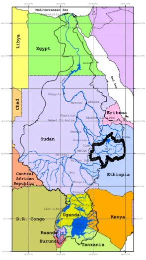
The Nile River (Fig. 1) travels more than 6500 km from its most remote source, at the headwaters of the River Kagera, the main feeder of Lake Victoria, till it discharges to the Mediterranean Sea (Shahin,1985). The Nile is an international river that traverses, with its tributaries, a total of ten countries: Tanzania, Uganda, Rwanda, Burundi,

Demo-5

cratic Congo (formerly Zaire), Kenya, Ethiopia, Eritrea, Sudan, and Egypt. The Nile has played a major role in shaping the region since the ancient Egyptian civilization. The Nile flood provided the necessary conditions for settlement based on agriculture in the Nile Valley and Delta. The Blue Nile is one of the most important tributaries of the Nile as it is the main responsible for the Nile flood contributing about 60% of the total Nile

10

yield.

This research focuses on the upper catchment of the Blue Nile which extends from 7◦₄₅′ _{to 13}◦_{N and 34}◦₃₀′ _{and 37}◦₄₅′_{E. The flow analysis has been performed for}

the Diem station, the outlet of the Upper Blue Nile basin (highlighted in Fig. 1) which covers an area of about 184 245 km2. This sub-basin is characterized by a highly

sea-15

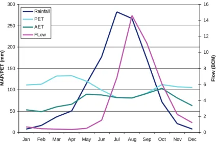
sonal rainfall pattern with most of the rainfall falling in four months (June to September – JJAS) with a peak in July or August (Fig. 2). The mean annual total rainfall for the 1961–1990 period amounts to 1224 mm, of which more than 70% fall within those four months. Flow lags one month behind rainfall peaking mostly in September with an average annual of 46.17 BCM (billion cubic meters) for the same period. PET

(calcu-20

lated using Penman-Monteith from CRU data as explained in the following sections) is higher during the dry season (December to April) than in the wet season due to increased cloudiness and humidity associated with rainfall. The total annual PET has been estimated as 1289 mm. However, actual evapotranspiration (AET) calculated us-ing the NFS hydrological model, only equals PET in the wet season when there is

25

enough moisture in the soil and thus it only amounts to 906 mm (about 70% of PET). The average runoff/rainfall coefficient of the basin is about 20% which means that 80% of the rainfall is lost to evaporation indicating the importance of this element in the water

(7)

HESSD

5, 1407–1439, 2008

Printer-friendly Version Interactive Discussion balance of the basin.

3 Datasets

Daily rainfall data from 17 different GCMs using the SRES A1B emission scenario (

Na-kicenovic and Swart,2000) have been obtained from the IPCC archive at the PCMDI website (http://www-pcmdi.llnl.gov/) for the period 2081–2098. In addition, the daily

5

data for the baseline period of 1961–1990 has been also obtained. This is the period for which most climate centers have submitted daily data for the 20th century climate experiment (20c3m). For the calculation of PET, monthly data of mean temperature, humidity, cloud cover, and wind speed for the same GCM experiments were obtained for both periods. Table 1 provides information about the 17 GCMs used in the study.

10

The observed rainfall dataset has been obtained from the NFS database as gridded rainfall fields for the period 1992–2006. These fields were created by merging satellite-based and gauge-satellite-based gridded fields of rainfall estimates using a spatially fixed set of monthly weights. Half hourly infrared images received from the METEOSAT satellite give the cloud-top temperature. These are used to infer rainfall assuming that very cold

15

temperatures correspond to very high clouds, which in turn are associated with rain-fall. The cloud-top temperature is thus used to delineate rainfall areas using a thresh-old temperature of −40◦C. The daily rainfall rate over a pixel is calculated as a linear function of the Cold Cloud Duration (CCD). That is the duration for which that pixel is covered with a cold cloud computed by accumulating all the half-hourly counts. Initially,

20

existing satellite estimation methods at the time of NFS development were investigated for use within the NFS including the GOES Precipitation Index (GPI) (Arkin, 1979) the READING technique (Milford and Dugdale,1990), the PERMIT technique (Barrett

et al.,1989), the Convective-Stratiform Technique (CST) (Adler and Negri,1988), and the Progressive Refinement Technique (PRT) (Bellerby and Barrett,1993). Currently

25

satellite rainfall is estimated by the Nile Hybrid technique (Green-Newby,1992,1993) which merges strengths of the CST and PRT Techniques to form a strategy designed

(8)

HESSD

5, 1407–1439, 2008

Printer-friendly Version Interactive Discussion to combine short-term and long-term satellite rainfall estimates to produce a high

res-olution (20 km) rainfall estimate.

Gauge estimates are obtained using the Nile Inverse Distance (NID) interpolation

(Cong and Schaake, 1995) technique based on WMO synoptic gauge data

down-loaded daily from the Internet. The NID is a variant of the inverse distance method

5

in which rainfall at an ungauged location is estimated as the weighted average of rain-fall at surrounding gauges where weights are the inverse distance between the gauges and the ungauged location (which are selected here to fall on the same grid as the satellite estimate). The NID blends that estimate with the long-term mean rainfall at the ungauged location to increase the influence of climatic characteristics for locations far

10

from gauges. This is similar to the climatologically aided interpolation (CAI) technique

ofWillmott and Robeson(1995). Note that not all stations send data continuously and,

on any particular day, usually data from about 40 stations are available. These are not necessarily the same ones received on another day. The observed daily database has 236 entries while only 142 of these lie within or close to the basin.

15

Regarding potential evapotranspiration (PET), the NFS originally used a set of 12 gridded monthly climatological fields based on data from FAO (LNDFC,2005) but the period and the data used to create these fields could not be traced from the docu-mentation. For the purpose of this study, a new PET climatology was created based on the available data from the Climatic Research Unit of the University of East Anglia

20

(CRU TS 2.1 –Mitchell and Jones,2005). This dataset comprises monthly time series of rainfall, temperature, diurnal temperature range, vapor pressure, cloud cover, wet day frequency, and frost day frequency for global land areas gridded at a resolution of 0.5◦. PET climatology for 1961–1990 has been calculated using the Penman-Monteith (P-M) method (Allen et al., 1998) based on temperature, diurnal temperature range,

25

vapour pressure, and cloudiness data. The calculations required the use of wind data and as these were not available as a time series, climatological values from the CRU CL 1.0 (New et al.,1999) were used. The CRU dataset is the only observed dataset available, to our knowledge, with all the necessary variables to calculate PET using the

(9)

HESSD

5, 1407–1439, 2008

Printer-friendly Version Interactive Discussion Penman-Monteith method.

The last dataset used in this research was the flow time series at Diem for the period 1961–1990. Flows started to be recorded at Roseries in 1912 but the gauging station had to be moved about 136 km upstream to Diem in 1961 for the construction of the Roseries Dam. A daily record is available for Diem in the NFS database starting May

5

1965 and this was collated with the record at Roseries to build a monthly time series for Roseries/Diem (referred to as Diem from now on) for the baseline period. The mean annual total flow at Diem for 1961–1990 amounts to 46.17 BCM.

4 Methodology

This study uses a distribution mapping approach to bias correct the intensity of daily

10

precipitation. Methods for mapping one distribution onto another are well established in probabilistic modeling and it has been used to correct the bias of both monthly and daily GCM precipitation data (Wood et al.,2002;Ines and Hansen,2006). Ideally one would correct both the frequency and intensity of precipitation. However, in order to preserve the climate change signal only the intensity was corrected. The basic procedure follows

15

that ofInes and Hansen(2006).

The observed dataset is chosen to be the merged satellite-gauge estimates obtained from the NFS database which is available for the period 1992–2006 at a fine resolution of 20×20 km2. A gamma distribution is fitted to the daily data (separately for each month) of the observed data and the GCM data for the baseline period. The distribution

20

of the GCM data is then adjusted to resemble that of the observed data. Several pixels of the fine resolution NFS fall into one large gridbox of the GCM and thus, the adjustment is repeated for each pixel resulting in a high resolution downscaled rainfall field. Although the observed dataset does not overlap with the 1961–1990 baseline period, it is the historical period available with near-observed daily data, especially

25

satellite data. Besides, the effect of this difference on the results has been found to be small as there is little difference in the mean monthly distribution for the two periods.

(10)

HESSD

5, 1407–1439, 2008

Printer-friendly Version Interactive Discussion For future scenarios, the climate signal (difference between future and baseline

cli-mates) is first removed before the distribution is adjusted. Note that we use a correction factor that takes into account changes in variability between the control and scenario simulation. Then, the climate signal is added back to create a rainfall scenario for the future. The extent to which this method preserves the relative rainfall change

sig-5

nal is assessed by comparing the percentage changes in rainfall before and after the correction as will be discussed in the results.

A PET climatology was calculated from the CRU dataset using the Penman-Monteithmethod for the 1961–1990 period as explained above (hereafter referred to as observed). As these are climatological monthly data, the approach of fitting a

dis-10

tribution was not applicable. Monthly gridded correction factors have instead been calculated as ratios of the observed climatology and that calculated for GCMs for the baseline period using the same method. These factors were then applied to future cli-matological monthly PET fields (2081–2098). A monthly time series of PET fields could have been also generated but a test using time series for the CRU dataset and for a

se-15

lected GCM showed that the mean hydrograph of the Blue Nile flow is not sensitive to interannual variability of PET. This has generally been reported for several hydrological models (e.g.Oudin et al.,2005).

The rainfall and PET inputs were then used to drive the NFS hydrological model. The NFS is a real-time distributed hydro-meteorological forecast system designed for

20

forecasting Nile flows at designated key points within the Nile. Of major interest is the inflow of the Nile into the High Aswan Dam, Egypt. The system is hosted at the Nile Forecasting Center (NFC) of the Ministry of Water Resources and Irrigation (MWRI), Giza, Egypt, which kindly provided a copy of the NFS software (version 5.1 NFC, 2007) and the available documentation for this research.

25

The core of the NFS is a conceptual distributed hydrological model of the whole Nile system including soil moisture accounting, hillslope and river routing, lakes, wet-lands, and man-made reservoirs within the basin. The main inputs to this model are the rainfall and potential evapotranspiration. The system relies on satellite-based

(11)

(ME-HESSD

5, 1407–1439, 2008

Printer-friendly Version Interactive Discussion TEOSAT) methods to estimate rainfall merged with gridded (to the METEOSAT grid)

gauge estimates from freely available sparse gauge data. All rainfall data is stored in the Nile Basin Hydro-meteorological Information System (NBHIS) which also holds flow records at all key river gauges. For more details on the NFS including an evaluation of its performance for long term simulations refer to (Elshamy,2006).

5

5 Results and analysis

In the following section, results based on scenario SRES A1B from 17 GCMs are used to illustrate the value of the method and to investigate the climate change impacts on the upper Blue Nile flow at Diem. Rainfall, PET, and AET are summarized as mean areal averages over the basin area. First, the sensitivity of the basin flow to climatic

10

drivers (rainfall and PET) is analyzed. An assessment of the ability of the bias cor-rection method to preserve the climate signal is then presented. Then, the quality of baseline simulations using the bias corrected rainfall and PET are assessed before future changes for the study basin are discussed. Finally, the different relationships between the flow and the main drivers are explored for the ensemble of models in an

15

attempt to provide more insight into the implications of climate change. 5.1 Sensitivity analysis

The Blue Nile has been shown by several authors to be sensitive to changes in both precipitation and PET (e.g.Conway and Hulme,1993;Sayed,2004). Both studies in-dicated that a 10% change in precipitation could yield more than 30% change in flow.

20

Sensitivity to PET was shown to be smaller (Conway and Hulme,1993). Driving the NFS with the baseline (1961–1990) PET climatology estimated from CRU data and monthly rainfall fields stored within the NFS database (based on gauge data), simi-lar results have been obtained for changes between ±30% for both variables (rainfall and PET) stepping 5% at a time while the other is kept constant. Flow response to

(12)

HESSD

5, 1407–1439, 2008

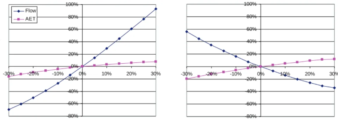
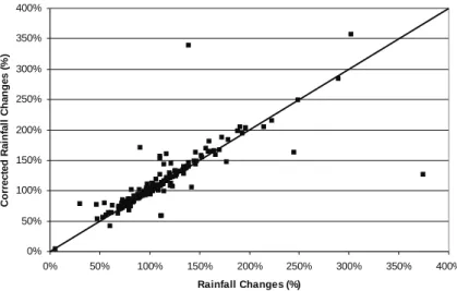
Printer-friendly Version Interactive Discussion rainfall changes deviates a little from being linear (Fig. 3) as it increases more rapidly

with increases in rainfall because AET is generally satisfied during the wet season (June–September) (see Fig. 2) and thus additional rainfall is directly translated to runoff. Reductions in rainfall reduce both flow and AET during the wet season and thus the change in flow to rainfall reduction is smaller than that for an increase of the same

mag-5

nitude (e.g. a 20% increase in rainfall yields 60% increase in flow while a 20% rainfall reduction yields 50% flow reduction). On the other hand, increasing PET by 30% in-creases AET by only 12% because inin-creases in the dry season are much smaller due to reduced moisture availability and thus AET becomes much higher in the wet season causing larger percentage reductions in flow (34% in the given case). A more

substan-10

tial response is shown for PET reductions as AET is reduced during the wet season causing large flow increases (flow increase of 56% for a 30% PET reduction).

During this sensitivity exercise, the importance of the absolute values of PET during the wet season (Fig. 2) became evident as this is when PET is always satisfied. In terms of magnitude, it was found that CRU-based PET had to be increased by 10%

15

to obtain a reasonable agreement between simulated and observed flows for Diem. Repeating the rainfall sensitivity exercise for this new baseline PET increases the sen-sitivity as the changes are calculated relative to a lower flow value but the general observations given above remain unchanged. Results given below are thus based on the 10% inflated CRU-based PET being used as the observed PET climatology for

cor-20

recting GCM bias. This factor might be accounting for the different vegetation type (as compared to grass which is the reference crop in the FAO Penman-Monteithmethod) or compensating for the use of standard coefficients in the Angstrom formula which relates solar radiation to extraterrestrial radiation and relative sunshine duration (refer

toAllen et al.,1998, for more information).

25

5.2 Bias corrected rainfall

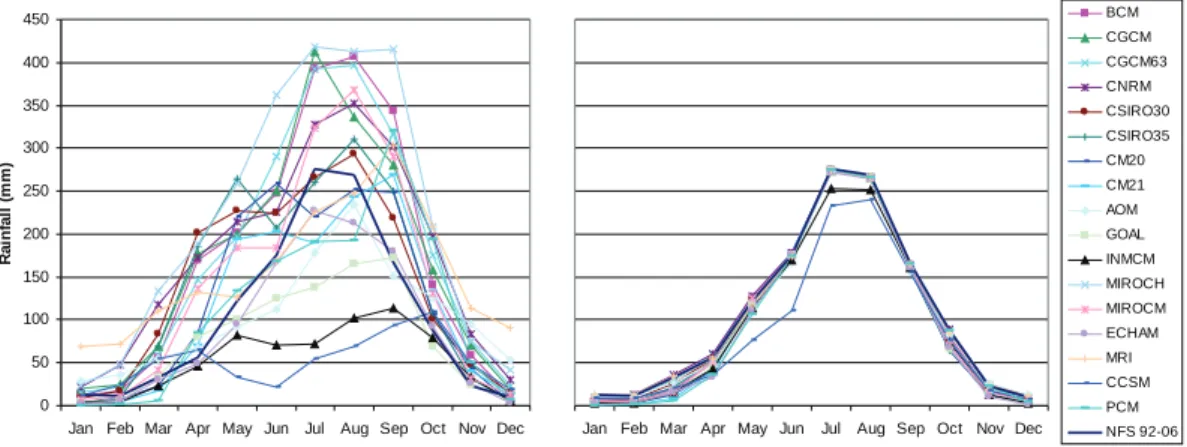
Figure 4 shows the mean distributions of rainfall from the 17 GCMs for the upper Blue Nile basin for the baseline period (1961–1990) before and after bias correction. It is

(13)

HESSD

5, 1407–1439, 2008

Printer-friendly Version Interactive Discussion evident that many of the models either overestimated or underestimated the rainfall

while some of the models were unable to reproduce the seasonal cycle. The cor-rection scheme brings the distributions close to the observed pattern (denoted NFS 92-06) except for CCSM and INMCM which originally had too low and somewhat bi-modal rainfall patterns. Notably, the scheme also preserves the climate change signal

5

(% change) for most models/months as depicted in Fig. 5. A few large deviations occur in the dry season when the gamma distribution assumption becomes less appropriate and the number of points used to fit it becomes small for some models/months. How-ever, these deviations have no or little effect on flow as they occur away from the wet season. It should be noted that biases in wet day frequencies are not corrected. This

10

gives a poorer correction for the baseline period, but more accurate conservation of the model’s original climate signal. For PET, the ratio-based bias correction is more exact and the points are concentrated around the 1:1 line (not shown).

5.3 Baseline simulations

Using the bias corrected rainfall from the 17 GCMs and the 10% inflated CRU-based

15

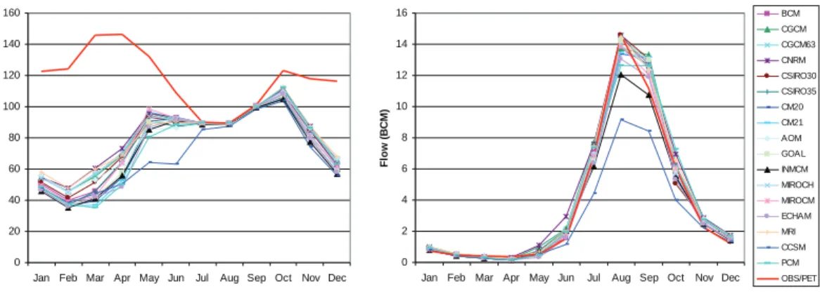
PET, the NFS was used to simulate the flow and AET time series for the baseline pe-riod 1961–1990. Most simulations were satisfactory with R2(Nash-Sutcliffe Efficiency) for the monthly time series ranging between 0.59 and 0.85 except for GOAL which had a relatively low R2of 0.49. RMSE ranged between 1.88 and 3.45 BCM which amounts to about 4.1–7.5% of the mean observed annual total. More important to this study,

20

is the simulation of the mean annual hydrograph (Fig. 6) as all models had small vol-ume biases of ±10% of the mean annual total except of the CCSM which had a high negative bias of about 29% and CNRM with a relatively high positive bias of 13%. The rainfall bias correction was less successful for the CCSM and the INMCM models as mentioned above and this remaining bias was amplified in the flow simulations with

25

large negative bias for the CCSM. In case of AET, the ensemble is packed specially for the wet season when AET from all models becomes equal to PET. The main deviation from the pack is observed for the CCSM model again due to its severe

(14)

underestima-HESSD

5, 1407–1439, 2008

Printer-friendly Version Interactive Discussion tion of rainfall both before and after correction. The results from this model are thus

handled with more care.

A test was done to see if the climate signal translated into flows is sensitive to the quality of their baseline simulation. For this purpose, all baseline simulations were re-peated using the correction factors based on the original CRU-based PET (i.e. without

5

the 10% inflation) which resulted in overestimating the flow for the baseline period from most models. The same correction factors were used for the future period and it was found that the direction of change (i.e. increase or reduction) was preserved and the magnitude (difference between future and baseline) remained similar. To avoid the bi-ases in flow results contaminating the climate signal, future changes for each model

10

were calculated with respect to the baseline simulation of that model for this test and for the results reported below.

5.4 Rainfall and PET changes

In terms of temperature, there is a consensus between all models that it will increase in the 2081–2098 period compared to the baseline period but with values ranging

be-15

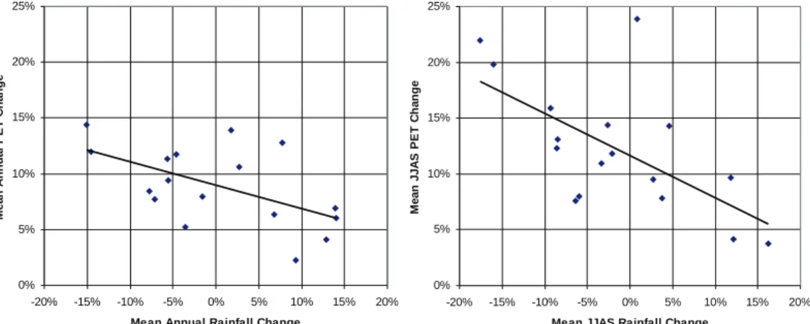
tween 2◦C and 5◦C annually. In turn, all GCMs report increases in total annual PET varying from +2 to +14%. However, the PET increase in not uniform throughout the year and thus the importance of PET changes will depend on how much of it is pre-dicted during the wet season. In agreement with all previous studies of the basin, GCMs disagree on the direction of precipitation change (Fig. 7) for the 2081–2098

pe-20

riod compared to the baseline. Changes in total annual precipitation range between −15% to +14% but more models report reductions (10) than those reporting increases (7). However, several models (6) report small changes within 5%. The largest reduc-tions are reported by the CM20 and CM21 experiments while the largest increases are reported by MIROCM and INMCM. The ensemble mean of all models shows no

25

change in the annual total rainfall and a very slight reduction (2.4%) in the wet season total. This should be interpreted with care as some models are less skilful than others in reproducing the baseline seasonal pattern of rainfall. The ensemble mean for the

(15)

HESSD

5, 1407–1439, 2008

Printer-friendly Version Interactive Discussion baseline period was about 6% and 2.2% lower than the observed for the annual and

wet season totals respectively.

There is a tendency of having smaller PET increases with increased rainfall which may be explained by increased cloudiness and humidity (Fig. 7). However, this re-quires further investigations as most models report cloudiness reductions in the future

5

compared to the baseline. This indicates that rainfall could be more intense in the fu-ture with possible implications of more flooding. Figure 7 shows a steeper relationship between rainfall and PET changes during the wet season. JJAS rainfall corresponds to 67–78% of the annual total and thus changes in JJAS rainfall are similar to changes in the annual total. On the other hand, JJAS PET corresponds to only 27–30% of the

10

annual total and most models report larger PET increases in the wet season compared to the change in the annual total which resulted in this steeper slope. However, both the annual and wet season relationships are not strong and have a lot of scatter due to changes in other PET variables (temperature, windspeed, etc.).

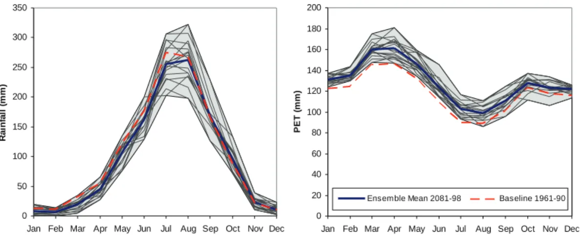
Figure 8 shows the mean monthly distributions of Rainfall and PET for the model

15

ensemble for the 2081–2098 period in comparison to the baseline distributions of the two variables. For rainfall, there is a little shift in most models towards more rainfall in August and less in July with some delay for the rising limb of the distribution but the general shape remains consistent with the baseline. For PET, there are higher in-creases in the January–July period than that occurs in the remainder of the year. Some

20

models (e.g. CNRM, GOAL) even report PET reductions in the August-December pe-riod. These changes may have some implications on the shape of the hydrograph as will be shown in the next section.

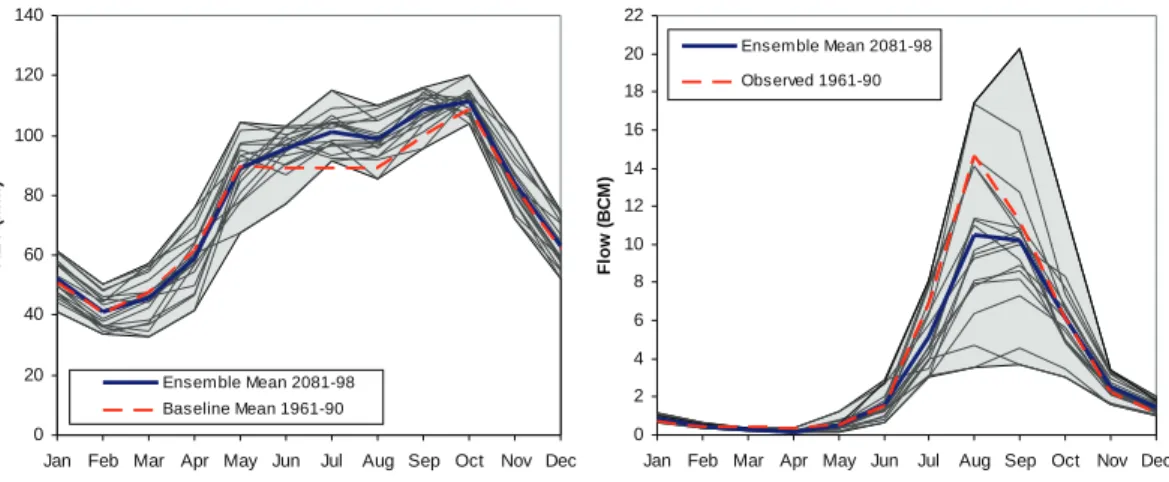
5.5 Flow and AET changes

Changes in AET generally followed that of PET during the wet season but have been

25

moderated by rainfall during the remainder of the year. The change in the annual total ranged from −2% for the CGCM and CGCM63 to 11% for CCSM but ranged from 1% to 18% for the wet season. Figure 9 shows a distinct increase in the ensemble

(16)

HESSD

5, 1407–1439, 2008

Printer-friendly Version Interactive Discussion mean during the wet season. A feedback seems to exist between the rainfall and AET

during the wet season that enhances the rainfall signal as depicted in Fig. 7. Models with large rainfall reductions tend to have large PET increases and therefore dramatic flow reductions. Given the high sensitivity of the flow to uniform changes in rainfall (PET) (see Sect. 5.1) when PET (rainfall) is kept constant, changes will be higher if

5

one variable strengthens the effect of the other.

This led to much more dramatic changes in flows with increases up to 45% for MIROCM and reductions up to 60% for CGCM63. There are more models showing flow reductions (11) than those showing increases (6) because all models showed in-creases in PET during the wet season and this counterbalanced small inin-creases in

10

rainfall from some models leading to overall flow reductions. Flow increased signifi-cantly only for those models with large rainfall increases (e.g. MIROCM, INMCM, and CCSM). Models with modest rainfall increases (within 10%) produced either small in-creases in flow (e.g. GOAL and AOM) or even reductions depending on how their PET changed. In general, the hydrograph (Fig. 9) shows a shift towards a more flat peak

15

extending till September with a slower rising limb. 5.6 Simple estimation of climate change impacts

Figure 10 attempts to separate the effects of future changes in PET and rainfall on flow. There seems to be a linear relationship between rainfall changes as depicted by the different GCMs and flow changes on annual basis and for the wet season (with a

20

one-month lag for flow). The slope of the relationship is steep (3.01) for the annual total and even steeper (3.25) for the wet season which means that changes in rainfall are amplified by a factor of three in flows. The fitted lines are nearly parallel to the sensitivity results where PET was held constant, which indicates that PET only changes the slope of the line slightly but it mainly shifts it down (i.e. towards less flow) by 14% for the

25

annual total and by 10% for the wet season. These results can be used to obtain rough estimates for the flow response of the upper Blue Nile basin to future changes in rainfall and PET.

(17)

HESSD

5, 1407–1439, 2008

Conway and Hulme (1996) assumed a 4% increase in PET per degree change in

temperature based on the results of other earlier studies. Figure 11 verifies that this assumption was a good one as the least-squared fit through the model ensemble re-sults has a similar slope (3.75% per◦C). However, there are still some outliers, e.g. GOAL predicts too little increase in PET for a very similar temperature change for which

5

CSIRO30 predicts a much higher increase. This is the role of other climatic variables such as wind speed and humidity and how they change in the future. The magnitude of PET is of higher importance during the wet season where it gets satisfied. For this period, the linear assumption seems to remain valid (Fig. 11) as well but at a steeper slope (5.6% increase in PET/◦C). The steeper slope during the wet season indicates a

10

higher role of the radiation component of PET, for which temperature acts as a surro-gate, during the wet season when the effect of cloudiness on PET is dominant. Models deviate from the least-squared fit due to the effect of other climatic variables on PET. Therefore, using a temperature-based method would probably give the general trend of the results in terms of PET change but would not provide the same level of detail

15

when models are analysed individually.

6 Conclusions

The upper Blue Nile basin is highly sensitive to both precipitation and evaporation changes. Changes are amplified by a factor of 2.9 for rainfall and by a factor of 1.4 for PET. Flow sensitivity to PET changes is dependent on rainfall as it is only satisfied

20

during the wet season when there is enough moisture in the soil. Under constant rainfall, flow becomes more sensitive to reductions in PET than to increases.

A probabilistic bias-correction method was applied to obtain fine-scale rainfall fields required by the NFS hydrological model. The method was capable of correcting most errors in the baseline climate reproducing the main features of observed rainfall in the

25

study region. The scheme removed the bias nearly completely for 15 out of 17 GCMs despite the fact that some models were not able to capture the seasonal cycle. The

(18)

HESSD

5, 1407–1439, 2008

Printer-friendly Version Interactive Discussion hydrological model were thus able to simulate the response of the sub-basin from most

models in close correspondence with the observed flow series at Diem. Additionally, the impact of a new PET climatology was assessed for the 1961–1990 baseline period. Notably, the bias correction method also preserved the models’ original climate change signal on a monthly time scale. This is a feature that is often distorted after simpler bias

5

correction methods.

The 17 GCMs show a large spread in their precipitation projections for 2081–2098 in the SRESA1B scenario. Some models predict large reductions up to 15%, others predict large increases up to 14% but most models predict modest changes (within 5%). The ensemble mean for all models shows almost no change in the total annual

10

volume but a slight shift towards a delayed peak. All models predict the temperature to increase between 2◦C and 5◦C, and consequently PET to increase by 2–14%. There is some evidence that higher reductions in rainfall may be accompanied by higher increases in PET, especially during the wet season, possibly due to higher reductions in cloud cover. This further enhances the effect of rainfall reduction on runoff leading

15

to very high reductions in the mean annual flow for some models (up to 60%). For models predicting small increases in rainfall, the increase in PET usually offsets this change resulting in small reductions in flow. Flow only increases (up to 45%) when the increase in rainfall is large enough to exceed the effect of PET increase. Therefore, more models are predicting reductions in flow than those showing increases. However,

20

the high uncertainty associated with this part of the Nile Basin remains unresolved, complicating water policy and management for the eastern Nile countries (Ethiopia, Sudan, and Egypt) and indicating the need of more research to enhance GCMs or test RCMs for the region.

Finally, simple relationships between changes in temperature, PET, precipitation, and

25

flow have been developed. They enable simple estimation of climate change impacts on the study basin and facilitate comparison with other modeling studies. This was achieved through the relatively large ensemble of GCMs used. PET changes were found to have a strong linear relationship with temperature changes. PET increases by

(19)

HESSD

5, 1407–1439, 2008

Printer-friendly Version Interactive Discussion 3.8% (annually) and 5.6% (wet season) per◦_{C warming. Additionally, PET increases}

mainly shift down the rainfall-flow change relationship (by 14% and 10% for the annual and wet season totals respectively) rather than changing its shape. Flow changes can thus be estimated roughly based on temperature and precipitation changes as has been done in many other studies. However, using the more sophisticated

Penman-5

Monteith method, this research illustrated the validity of these relationships and showed that they are also prone to deviations as other climate variables (cloudiness, humidity, and wind speed) play their roles in changing PET. Additional research is underway to quantify the respective effects of these variables on PET.

It should be noted that the use of relatively short reference and scenario periods

10

(30 and 20 years, respectively) make the across model spread in climate signal a function of both real differences in the models’ response to greenhouse gas changes and differences due to insufficient sampling of the models decadal climate variability. The across-model differences should therefore not be interpreted only as real model differences. The influence of using relatively short reference and scenario periods is

15

discussed in details inSorteberg and Kvamsto(2006).

Acknowledgements. This research was done under the Nile Basin Research Programme (NBRP), hosted at the University of Bergen, Norway during Autumn 2007 and Spring 2008. We thank Semu Moges for valuable comments to a draft of this manuscript. We acknowledge the modeling groups, the Program for Climate Model Diagnosis and Intercomparison (PCMDI) 20

and the WCRP’s Working Group on Coupled Modelling (WGCM) for their roles in making avail-able the WCRP CMIP3 multi-model dataset. Support of this dataset is provided by the Office of Science, US Department of Energy. The Nile Forecast Center, Ministry of Water Resources and Irrigation of Egypt is acknowledged for providing the Nile Forecast Center software and documentation.

25

References

Adler, R. and Negri, A.: A satellite infrared technique to estimate tropical convective stratiform

(20)

HESSD

5, 1407–1439, 2008

Allen, R. G., Pereira, L. S., Raes, D., and Smith, M.: Crop evapotranspiration: Guidelines for computing crop water requirements, FAO Irrigation and Drainage Paper No. 56, Food and

Agriculture Organization of the United Nations, Rome, 1998. 1410,1413,1417

Arkin, P. A.: The Relationship between Fractional Coverage of High Cloud and Rainfall Accu-mulations during GATE over the B-Scale Array, Mon. Weather Rev., 107, 1382–1387, 1979. 5

1412

Arnell, N. W.: A simple water balance model for the simulation of streamflow over a large

geographic domain, J. Hydrol., 217, 314–335, 1999. 1409

Barrett, C. B., Richards, T. S., Rangoonwala, A., Ahmed, S., Huk, S., and Mirza, M. I.: Towards

an operational system for the use of AVHRR data in Pakistan, 1989.1412

10

Bellerby, T. J. and Barrett, E. C.: Progressive Refinement - a Strategy for the Calibration by Collateral Data of Short-Period Satellite Rainfall Estimates, J. Appl. Meteorl., 32, 1365–1378,

1993. 1412

Cong, S. and Schaake, J.: Test on the Approximation of the Distribution Transformation in the W-K Method and its influence on the MAP Estimation, Tech. Rep. No. 0032.2, Nile Forecast 15

Center, Ministry of Water Resources and Irrigation, 1995. 1413

Conway, D. and Hulme, M.: Recent fluctuations in precipitation and runoff over the Nile

sub-basins and their impact on main Nile discharge, Climatic Change, 25, 127–151, 1993. 1416

Conway, D. and Hulme, M.: The Impacts of Climate Variability and Future Climate Change in the Nile Basin on Water Resources in Egypt, Int. J. Water Resour. Develop., 13, 277–296, 20

1996. 1410,1421

Elshamy, M. E. A. M.: Impacts of climate change on Nile flows, Diploma of imperial college

(DIC), Imperial College London, 2000. 1409

Elshamy, M. E. A. M.: Improvement of the Hydrological Performance of Land Surface Param-eterization: An Application to the Nile Basin, Doctor of philosophy (PhD), Imperial College, 25

University of London, 2006.1416

Green-Newby, J. L.: Nile Hydrid Technique for Version 2.0, Tech. Rep. No. 0074, Nile Forecast

Center, Ministry of Water Resources and Irrigation, 1992. 1412

Green-Newby, J. L.: Satellite Rainfall Estimation Techniques, Tech. Rep. No. 0075, Nile

Fore-cast Center, Ministry of Water Resources and Irrigation, 1993.1412

30

Hewitson, B. C. and Crane, R. G.: Climate downscaling: Techniques and application, Climate

Research, 7, 85–95, 1996. 1408

(21)

HESSD

5, 1407–1439, 2008

studies, Agr. Forest Meteorol., 138, 44–53, 2006. 1414

IPCC: Climate Change 2007: The Physical Science Basis – Summary for Policy Makers: Con-tribution of Working Group I to the Fourth Assessment Report of the Intergovernmental Panel

on Climate Change,www.ipcc.ch, 2007.1410

LNDFC: Impact of Climate Change on the Water Supply to Egypt, Tech. rep., Ministry of Water 5

Resources and Irrigation, Nile Forecasting Center, Lake Nasser Flood and Drought Control

Project (LNDFC/ICC), 2005. 1413

Milford, J. R. and Dugdale, G.: Estimation of rainfall using geostationary satellite data, in: Applications of remote Sensing in Agriculture, edited by: Steven, M. D. and Clark, J. A., Proceedings of the 48th Easter School in Agriculture Science, University of Nottingham, 10

Butterworth, London, 97–110, 1990. 1412

Mitchell, T. and Jones, P.: An improved method of constructing a database of monthly climate

observations and associated high-resolution grids, Int. J. Climat., 25, 693–712, 2005. 1413

Nakicenovic, N. and Swart, R. (Eds.): Special Report on Emissions Scenarios., Cambridge

University Press, Cambridge, UK, 2000. 1412

15

New, M., Hulme, M., and Jones, P.: Representing Twentieth-Century Space-Time Climate Variability. Part I: Development of a 1961–1990 Mean Monthly Terrestrial Climatology, J.

Climate, 12, 829–856, 1999.1413

Nile Forecast Center: Nile Forecasting System version 5.1, Ministry of Water Resources and irrigation, Cairo, Egypt, 2007.

20

Oudin, L., Michel, C., and Anctil, F.: Which potential evapotranspiration input for a lumped rainfall-runoff model? Part 1 – Can rainfall-runoff models effectively handle detailed potential

evapotranspiration inputs?, J. Hydrol., 303, 275–289, 2005.1415

Sayed, M.-A.: Impacts of climate change on the Nile Flows, Ph.D. thesis, Ain Shams University,

2004. 1409,1416

25

Shahin, M.: Hydrology of the Nile Basin, Developments in water science ; 21, Elsevier,

Ams-terdam, Oxford, mamdouh Shahin., 1985. 1411

Sorteberg, A. and Kvamsto, N. G.: The effect of internal variability on anthropogenic climate projections, Tellus Series A-Dynamic Meteorology And Oceanography, 58, 565–574, 2006.

1424

30

Strzepek, K., Yates, D., Yohe, G., Tol, R., and Mader, N.: Constructing not implausible Climate

and Economic Scenarios for Egypt, Integrated Assessment, 2, 139–157, 2001.1409

(22)

HESSD

5, 1407–1439, 2008

methods and limitations, Progress in Physical Geography, 21, 530–548, 1997.1409

Willmott, C. J. and Robeson, S. M.: Climatologically Aided Interpolation (CAI) of Terrestrial

Air-Temperature, Int. J. Climat., 15, 221–229, 1995.1413

Wood, A. W., Maurer, E. P., Kumar, A., and Lettenmaier, D. P.: Long-range experimental hydrologic forecasting for the eastern United States, J. Geophys. Res., 107(D20), 4429, 5

doi:10.1029/2001JD000659, 2002. 1414

Yates, D. N. and Strzepek, K. M.: An assessment of integrated climate change impacts on the

(23)

HESSD

5, 1407–1439, 2008

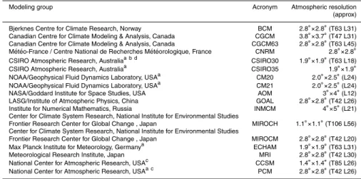
Printer-friendly Version Interactive Discussion Table 1. Information about the 17 GCMs from the IPCC 4th assessment report used in the

study.

Modeling group Acronym Atmospheric resolution

(approx)

Bjerknes Centre for Climate Research, Norway BCM 2.8◦

×2.8◦(T63 L31)

Canadian Centre for Climate Modeling & Analysis, Canada CGCM 3.8◦

×3.7◦(T47 L31)

Canadian Centre for Climate Modeling & Analysis, Canada CGCM63 2.8◦

×2.8◦(T63 L45)

M ét éo-France / Centre National de Recherches M ét éorologique, France CNRM 2.8◦_×2.8◦

CSIRO Atmospheric Research, Australiaa b d CSIRO30 1.9◦_×1.9◦_{(T63 L18)}

CSIRO Atmospheric Research, Australiaa CSIRO35 1.9◦

×1.9◦

NOAA/Geophysical Fluid Dynamics Laboratory, USAa CM20 2.0◦

×2.5◦(L24)

NOAA/Geophysical Fluid Dynamics Laboratory, USAa CM21 2.0◦_×2.5◦_(L24)

NASA/Goddard Institute for Space Studies, USA AOM 3◦×4◦(L12)

LASG/Institute of Atmospheric Physics, China GOAL 2.8◦

×2.8◦(T42 L26)

Institute for Numerical Mathematics, Russia INMCM 4◦

×5◦(L21)

Center for Climate System Research, National Institute for Environmental Studies

Frontier Research Center for Global Change , Japan MIROCH 1.1◦

×1.1◦(T106 L56)

Center for Climate System Research, National Institute for Environmental Studies

Frontier Research Center for Global Change , Japan MIROCM 2.8◦_×2.8◦_{(T42 L20)}

Max Planck Institute for Meteorology, Germanya ECHAM 1.9◦

×1.9◦(T63 L31)

Meteorological Research Institute, Japan MRI 2.8◦

×2.8◦(T42 L30)

National Center for Atmospheric Research, USAc CCSM 1.4◦_×1.4◦_{(T85 L26)}

National Center for Atmospheric Research, USAa c PCM 2.8◦

×2.8◦(T42 L26)

a_{These models did not provide 2 m specific humidity. Instead specific humidity at the lowest model level above orography were used. A test was performed}

using models having both variables (11 models). The effect on PET was absorbed in the calculated correction factors.

b_{The surface wind for 2081–2098 was missing. Instead the 1961-90 surface wind was used. Most models showed only small wind changes between the}

baseline and future periods.

c_{The surface wind was not provided. The CRU climatological wind fields, spatially averaged to model resolution, were used instead.}

(24)

HESSD

5, 1407–1439, 2008

Printer-friendly Version Interactive Discussion ! ! ! ! " # " " # # " # # " # ! ! " # # 7 7 7 7 7 7 7 7 7 7 7 7 7 7 7 7 7 7 7 7 7 7 7 7 7 7 7 7 7 7 7 7 7 7 7 7 7 7 7 7 7 7 777 7 7 7 7 7 7 7 7 7 7 7 7 7 7 7 7 7 7 7 7 7 7 7 7 7 7 7 7 7 7 7 7 7 7 7 7 7 7 7 7 7 7 7 7 7 7 7 7 7 7 7 7 7 77 7 7 7777777777777 7 7 7 7 7 7 7 7 7 7 7 7 777 7 7 7 7 7 7 7 7777777777777 7 7 7 7 7777777777777777777777777777777777777777777777777777777777777777777777777777777777777777777777777777777777777777777777777777777777777777777777777777777777777777777777777777777777777777777777777777777777777777777777777777777777777777777777777777777777777777777777777777777777777777777777777777777777777777777777777777777777777777777777777777777777777777777777777777777777777 7 7 77 !"#$ %&'()*&" +),$*&$, ! "_# !_$ " % &"#'("))%*"%*!$"% !" #$! -", ,$* !"#$!./0$*( $+#%* ,-!-!./*0/ 1 ' 2 3 % . 4 % # 5036( 5(4'/6'% 7"*3% 80%*#% !."*()%9 !:;)'<%* !"6+29'< 5)'()"% =%*>%*'% !?%*#% @+)+*#' 1)* 2&$3 4$/5( .,6"7 8"&*) 4"0&/ -&35/$ .(0"*" 9$77"* 4$*)6$ 4)7:)/" 2)7:)/" 4"/"#"/ ;<"*()53 ="#6"('< >&7?" ./$@"7A*&" !"#$!B"7" C$0$/!D/!.5/&" !"#$!;E):" ;<",<3!D/!C&*0" F&//$(!2)/$&0 GH"HIHJD GH"HIHJD KL"HIHJD KL"HIHJD KH"HIHJD KH"HIHJD ML"HIHJD ML"HIHJD L"HIHJ9 KH"HIHJ- KH"HIHJ-ML"HIHJ- ML"HIHJ-MH"HIHJ- MH"HIHJ-NL"HIHJ- NL"HIHJ-NH"HIHJ- NH"HIHJ-L"HIHJ- L"HIHJ-H"HIHJ H"HIHJ

(25)

HESSD

5, 1407–1439, 2008

Printer-friendly Version Interactive Discussion ! " "! # #! $

%&' ()* +&, -., +&/ %0' %01 -02 3). 456 789 :)5

!" #" $% &'( ( ) # ; < = " "# "; "< *+ ,-&'. / ) >&?'@&11 ABC -BC (D8E

(26)

HESSD

5, 1407–1439, 2008

Printer-friendly Version Interactive Discussion F= G F< G F; G F# G G # G ; G < G = G " G F$ G F# G F" G G " G # G $ G 0&123452++&/62478 0 &* +, -#! $% &/ 62 47 8& (18E -BC F= G F< G F; G F# G G # G ; G < G = G " G F$ G F# G F" G G " G # G $ G 0&"$%&/62478

Fig. 3. Mean annual flow and actual evapotranspiration (AET) response for the Upper Blue Nile

(27)

HESSD

5, 1407–1439, 2008

Printer-friendly Version Interactive Discussion ! " "! # #! $ $! ; ;!

%&' ()* +&, -., +&/ %0' %01 -02 3). 456 789 :)5

12 34 52 ++& '( ( )

%&' ()* +&, -., +&/ %0' %01 -02 3). 456 789 :)5 HI+ IJI+ IJI+<$ I7>+ I3K>4$ I3K>4$! I+# I+#" -4+ J4-D K7+I+ +K>4IL +K>4I+ BIL-+ +>K II3+ AI+ 7(3MN#F <

Fig. 4. Mean monthly distributions of precipitation for the Upper Blue Nile Basin for 1961–1990

(28)

HESSD

5, 1407–1439, 2008

Printer-friendly Version Interactive Discussion G ! G " G "! G # G #! G $ G $! G ; G G ! G " G "! G # G #! G $ G $! G ; G 123452++&/624789&'0) /, :: 8; <8 =& 12 34 52 ++& /6 24 78 9& '0 )

Fig. 5. The change in rainfall between 1961–1990 and 2081–2098 for all months and models

(29)

HESSD

5, 1407–1439, 2008

Printer-friendly Version Interactive Discussion # ; < = " "# "; "<

%&' ()* +&, -., +&/ %0' %01 -02 3). 456 789 :)5

$> 2? ,: 2< 3, 4& '( ( ) # ; < = " "# "; "<

%&' ()* +&, -., +&/ %0' %01 -02 3). 456 789 :)5

*+ ,-&'. / ) HI+ IJI+ IJI+<$ I7>+ I3K>4$ I3K>4$! I+# I+#" -4+ J4-D K7+I+ +K>4IL +K>4I+ BIL-+ +>K II3+ AI+ 4H3OABC

Fig. 6. Mean monthly simulated distributions of AET and flow for 1961–1990. The thick red line

(30)

HESSD

5, 1407–1439, 2008

Printer-friendly Version Interactive Discussion G !G " G "!G # G #!G F# G F"!G F" G F!G G !G " G "!G # G 824&!44@2+&123452++&/62478 8 24 &! 44 @2 +&" $% &/ 62 47 8 G !G " G "!G # G #!G F# G F"!G F" G F!G G !G " G "!G # G 824&AA!B&123452++&/62478 82 4& AA !B &" $% &/ 62 47 8

Fig. 7. Projected changes in precipitation vs. changes in PET for the Upper Blue Nile Basin.

(31)

HESSD

5, 1407–1439, 2008

Printer-friendly Version Interactive Discussion ! " "! # #! $ $!

%&' ()* +&, -., +&/ %0' %01 -02 3). 456 789 :)5

12 34 52 ++& '( ( ) # ; < = " "# "; "< "= #

%&' ()* +&, -., +&/ %0' %01 -02 3). 456 789 :)5

"$ %& '( ( ) B'P)Q*1)M+)&'M# ="FN= H&P)1?')M"N<"FN

Fig. 8. Mean monthly precipitation and PET distributions for the Upper Blue Nile Basin for

2081–2098 as simulated by the 17 bias-corrected GCMs. The rainfall baseline is the observed 1992–2006 mean and baseline PET is the 10% Inflated CRU-based 1961–1990 climatology. The grey band shows the range of the different GCMs with light lines showing individual model results.

(32)

HESSD

5, 1407–1439, 2008

Printer-friendly Version Interactive Discussion # ; < = " "# ";

%&' ()* +&, -., +&/ %0' %01 -02 3). 456 789 :)5

!$ %& '( ( ) B'P)Q*1)M+)&'M# ="FN= H&P)1?')M+)&'M"N<"FN # ; < = " "# "; "< "= # ##

%&' ()* +&, -., +&/ %0' %01 -02 3). 456 789 :)5

*+ ,-&'. / ) B'P)Q*1)M+)&'M# ="FN= 4*P),9)RM"N<"FN

Fig. 9. Mean monthly AET and flow distributions for the Upper Blue Nile Basin for 2081–2098.

The grey band shows the range of the different models with light lines showing individual model results.

(33)

HESSD

5, 1407–1439, 2008

Printer-friendly Version Interactive Discussion STMUM$V " =MS>MFM V";W; >#_{MUM VN$W=} F" G G " G F# G G # G 824&!44@2+&123452++&/62478&'C1) 82 4& !4 4@ 2+ &* +, -&/ 62 47 8& 'C D ) HI+ IJI+ IJI+<$ I7>+ I3K>4$ I3K>4$! I+# I+#" -4+ J4-D K7+I+ +K>4IL +K>4I+ BIL-+ +>K II3+ AI+ STMUM$V#;W!MS>MFM V" # >#_{MUM VNW #} F" G G " G F# G G # G 824&AA!B&123452++&/62478&'C1) 82 4& A! BE &* +, -&/ 62 47 8& 'C D ) HI+ IJI+ IJI+<$ I7>+ I3K>4$ I3K>4$! I+# I+#" -4+ J4-D K7+I+ +K>4IL +K>4I+ BIL-+ +>K II3+ AI+

Fig. 10. Annual and wet season changes in flow vs. the corresponding changes in precipitation

for the Upper Blue Nile Basin Straight line indicates least-squared fit through GCM results. The dashed line shows the sensitivity curve from Fig. 2.

(34)

HESSD

5, 1407–1439, 2008

Printer-friendly Version Interactive Discussion SABCMUM V $W!MSCMFM V $W >#_{MUM V<N} G !G " G "!G # G #!G #V #V! $V $V! ;V ;V! !V !V! 824&!44@2+&%8(?8:2<@:8&/62478&'C%&F/) 8 24 &! 44 @2 +&" $% &/ 62 47 8& 'C "$ %) HI+ IJI+ IJI+<$ I7>+ I3K>4$ I3K>4$! I+# I+#" -4+ J4-D K7+I+ +K>4IL +K>4I+ BIL-+ +>K II3+ AI+ SABCMUM V !<MSCMFM V < >#_{MUM VW;} G !G " G "!G # G #!G #V #V! $V $V! ;V ;V! !V !V! 824&AA!B&%8(?8:2<@:8&/62478&'C%&F/) 82 4& AA !B &" $% &/ 62 47 8& 'C "$ %) HI+ IJI+ IJI+<$ I7>+ I3K>4$ I3K>4$! I+# I+#" -4+ J4-D K7+I+ +K>4IL +K>4I+ BIL-+ +>K II3+ AI+

Fig. 11. Annual and wet season (JJAS) changes in PET vs. changes in temperature for the