HAL Id: hal-03142211
https://hal.inria.fr/hal-03142211
Submitted on 15 Feb 2021
HAL is a multi-disciplinary open access
archive for the deposit and dissemination of
sci-entific research documents, whether they are
pub-lished or not. The documents may come from
teaching and research institutions in France or
abroad, or from public or private research centers.
L’archive ouverte pluridisciplinaire HAL, est
destinée au dépôt et à la diffusion de documents
scientifiques de niveau recherche, publiés ou non,
émanant des établissements d’enseignement et de
recherche français ou étrangers, des laboratoires
publics ou privés.
ALBA: a comprehensive growth model to optimize
algae-bacteria wastewater treatment in raceway ponds
Francesca Casagli, Gaetano Zuccaro, Olivier Bernard, Jean-Philippe Steyer,
Elena Ficara
To cite this version:
Francesca Casagli, Gaetano Zuccaro, Olivier Bernard, Jean-Philippe Steyer, Elena Ficara. ALBA: a
comprehensive growth model to optimize algae-bacteria wastewater treatment in raceway ponds.
Wa-ter Research, IWA Publishing, 2021, 190, pp.116734. �10.1016/j.watres.2020.116734�. �hal-03142211�
1
ALBA: a comprehensive growth model to optimize algae-bacteria
1
wastewater treatment in raceway ponds
2
Francesca Casaglia, Gaetano Zuccarob, Olivier Bernardc, Jean-Philippe Steyerb, Elena Ficaraa
3
4
a: Politecnico di Milano, Dip. di Ingegneria Civile e Ambientale (DICA), Piazza L. da Vinci, 32, 20133 Milan, Italy
5
b: INRAE, Univ Montpellier, LBE, 102 Avenue des étangs, Narbonne, France
6
c: Biocore, Univ Cote d’Azur, Inria, Sophia-Antipolis, France
7
8
*-Corresponding author: [email protected]
9
10
Abstract: This paper proposes a new model describing the algae-bacteria ecosystem evolution in an
11
outdoor raceway for wastewater treatment. The ALBA model is based on a mass balance of COD, C, N and
12
P, but also H and O. It describes growth and interactions among algae, heterotrophic and nitrifying bacteria,
13
while local climate drives light and temperature. Relevant chemical/physical processes are also included.
14
The minimum-law was used as ground principle to describe the multi-limitation kinetics. The model was
set-15
up and calibrated with an original data set recorded on a 56 m2 raceway located in the South of France,
16
continuously treating synthetic wastewater. The main process variables were daily measured along 443 days
17
of operations and dissolved O2 and pH were on-line recorded. A sub-dataset was used for calibration and the
18
model was successfully validated, along the different seasons over a period of 414 days. The model proved
19
to be effective in reproducing both the short term nycthemeral dynamics and the long-term seasonal ones.
20
The analysis of different scenarios reveals the fate of nitrogen and the key role played by oxygen and CO2 in
21
the interactions between the different players of the ecosystem. On average, the process turns out to be CO2
22
neutral, as compared to a standard activated sludge where approximately half of the influent carbon will end
23
up in the atmosphere. The ALBA model revealed that a suboptimal regulation of the paddle wheel can bring
24
to several detrimental impacts. At high velocity, the strong aeration will reduce the available oxygen provided
25
by photo-oxygenation, while without aeration, it can rapidly lead to oxygen inhibition of the photosynthetic
26
process. On the other hand, during night, the paddle wheel is fundamental to ensure enough oxygen in the
27
system to support algal-bacteria metabolism. The model can be used to support advanced control strategies,
28
including smart regulation of the paddle wheel velocity to more efficiently balance the mixing, aeration and
29
degassing effects.
30
31
Keywords: Modelling; Microalgae; Wastewater; Long-Term Validation; Raceway; Mass transfer rate
32
2
33
1. Introduction
34
The use of microalgae for wastewater treatment was first studied in the 50s (Oswald et al., 1957) and more
35
recently revisited, in view of a more sustainable and circular approach to bioremediation (Muñoz and
36
Guieysse, 2006; Cai et al., 2013). Indeed, when applied to wastewater treatment, these microscopic
37
photosynthetic organisms contribute to reduce the energy demand by supplying the oxygen through
38
photosynthesis. Moreover, microalgae assimilate inorganic nitrogen and phosphorus and thus participate to
39
the treatment process. Compared to classical activated sludge processes, algae will also recycle the carbon
40
dioxide produced by bacteria, reducing the greenhouse gas emissions (Arashiro et al., 2018). Moreover,
41
some algal species can contain high amounts of lipids, protein or other compounds that become elemental
42
bricks for green chemistry (Chew et al., 2017). Microalgae appear then as new players to recycle nitrogen
43
and phosphorus using the solar energy and providing useful products such as biofuel, bioplastics, or
bio-44
fertilizer (Uggetti et al., 2014, Arias et al., 2019).
45
However, challenges must still be addressed to benefit from the key advantages of involving microalgae in
46
wastewater treatment. Facing seasonal fluctuations of light and temperature is particularly difficult, especially
47
to keep an effective algal activity at low temperatures and light during winter. Moreover, promises of the
48
microalgae-based technology have rarely been quantified, mainly because most of the underlying processes
49
are not easily measurable. For example, the balance between oxygen production by photosynthesis,
50
consumption by bacterial respiration, and the role of the oxygen exchange with the atmosphere was never
51
fully assessed. On top of this, estimating the benefits and costs based on non-optimised pilots run over a
52
yearlong period is challenging and requires expensive field testing and data collection. All these open
53
questions can be effectively addressed with the support of numerical simulations once a reliable model is
54
made available (Shoener et al., 2019).
55
Mathematical models can indeed be used to quantify the mass and energy fluxes, and eventually optimise
56
the process from design to operation. An accurate model is a very powerful tool to identify the most efficient
57
operating modes, and then run an environmental or economic analysis. Modelling has demonstrated its
58
power in many fields of biotechnology, and especially in wastewater treatment where the ASMs and ADM1
59
models (Henze et al., 2000; Batstone et al., 2002) are currently used at industrial scale.
60
The challenge for microalgal based wastewater treatments is that currently, no comprehensive models have
61
been validated over a yearly period and applied to different case studies.
3
Designing and validating a mathematical model that would be able to keep a coherent behaviour despite the
63
nychthemeral and seasonal changes in light, temperature, rain and wind is indeed particularly challenging.
64
Up to now, only models describing bacteria-based systems for wastewater treatment were more extensively
65
studied and were indeed validated on longer time scales (Van Loosdrecht et al., 2015).
66
Few models have already been developed for simulating algae-bacteria interactions in outdoor systems. The
67
RWQM1 (Reichert et al., 2001) was developed for modelling wastewater discharge in a river, while
68
BioAlgae2 (Solimeno et al., 2019) describes the dynamics in a raceway reactor. Models are available for
69
simulating indoor reactors, as PHOBIA (Wolf et al., 2007) and the Modified ASM3 (Arashiro et al., 2017). A
70
recent detailed comparison among available algae models can be found in Shoener et al. (2019) and it has
71
been expanded for algae-bacteria models in Supporting Information (Table SI.11).
72
The aim of this work is to develop a global model, integrating the main chemical, physical and biological
73
processes taking place in outdoor systems of algae-bacteria consortia treating wastewater. The model which
74
was initially presented in Casagli et al. (2019) shares some common choices with the above cited
algae-75
bacteria models, in particular with the ones simulating outdoor environments (RWQM1 and BioAlgae2).
76
However, several aspects were modelled with a different/innovative approach, and especially: i) the
77
philosophy of biological kinetics in the ALBA model, that is based on the Liebig’s minimum law (De Baar,
78
1994); ii) the pH sub-model including a detailed chemical speciation and implemented by an algebraic
79
system; iii) the sensitivity analysis procedure, based on seasonal data elaborations and simulations; iv) the
80
conditions under which the model was calibrated and validated (including sub-optimal conditions, such as
81
winter); v) the evaluation of the evaporation process and of its effect on dissolved and suspended
82
compounds. A more detailed description and comparison of the modelling choices can be found in Section
83
5.1 and in Table SI.11.
84
The ALBA model describes growth and interactions among algae, heterotrophic and nitrifying bacteria,
85
accounting for carbon, nitrogen and phosphorous fluxes. Local climate drives light, temperature and
86
eventually the whole process dynamics. The model was developed balancing realism and complexity, so that
87
an efficient calibration procedure was possible. The key objective was to validate the model both on short
88
(nychthemeral) and long-term (seasonal) datasets. Fifteen months of an original field-testing campaign on an
89
outdoor demonstrative raceway pond treating a synthetic wastewater were then used for supporting model
90
calibration and validation along the four seasons.
91
The paper is structured as follows: first the experimental dataset is presented, then model structure and the
92
main hypotheses are explained. Nychthemeral simulations of pH and oxygen are compared to experimental
4
data. Long term predictions are compared with data from the monitoring campaign through the different
94
seasons. The key-role of oxygen and pH in microbial interactions is analysed. The fate of nitrogen within the
95
system is discussed and the actual role of microalgae for providing oxygen to bacteria is discussed in
96
comparison with the effect of the paddle wheel for aeration. Finally, the advantages of including microalgae
97
in the wastewater treatment process are quantified and discussed.
98
99
2. Material and methods
100
2.1. Experimental set up and data collection
101
The outdoor High Rate Algal Bacterial Pond (HRABP) of 17 m3 was located in Narbonne, France
(INRAE-102
LBE, Latitude: 43.15656, Longitude: 2.994438). The total surface area was 56 m2 with a length of 15 m and
103
a water depth of 0.3 m. The reactor was mixed with a paddle wheel (resulting linear velocity of 0.2 m s-1) and
104
an additional pump (flow rate 182 m3 d-1, located at the opposite side from the wheel).
105
The raceway was operated in chemostat mode, from 15/05/2018 to 01/08/2019. The inflow rate was set to
106
operate at an HRT of 5 days along the whole period, except from one month (29/08/2018-29/09/2018) during
107
which different HRT values (2 and 10 days) were tested. The outflow was implemented by gravity overflow.
108
The HRABP was equipped with dissolved oxygen (METTLER TOLEDO InPro 6850i), temperature and pH
109
(METTLER TOLEDO InPro4260(i)/SG/425) probes. In addition, data from an ultrasonic distance sensor
110
measuring the liquid level (Siemens, 7ML5221-1BB11) were available. Incident light at the reactor surface
111
was measured with a PAR probe (PAR 2625 SKYE). Online measurements were collected every five
112
minutes using the SILEX-LBE system (INRAE-LBE, France).
113
The reactor was inoculated with a microalgae suspension, where Chlorella sp. and Scenedesmus sp. were
114
the dominant algal species. It was fed on a synthetic medium, mimicking a municipal wastewater (Nopens et
115
al., 2001, Table 1), including complex organic nutrient sources (starch, milk powder, yeast, peptone). In this
116
wastewater, the main source of nitrogen is urea, while inorganic carbon comes from the tap water used for
117
influent dilution. Nitrite and nitrate concentrations were negligible (<0.3 mg L-1).
118
119
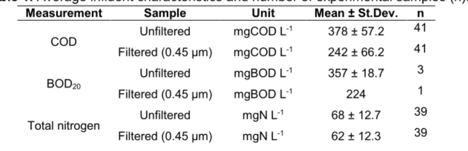
Table 1. Average influent characteristics and number of experimental samples (n).
120
Measurement Sample Unit Mean ± St.Dev. n
COD Unfiltered mgCOD L
-1 378 ± 57.2 41
Filtered (0.45 μm) mgCOD L-1 242 ± 66.2 41
BOD20
Unfiltered mgBOD L-1 357 ± 18.7 3
Filtered (0.45 μm) mgBOD L-1 224 1
Total nitrogen Unfiltered mgN L
-1 68 ± 12.7 39
5
P-PO4
3-Unfiltered mgP L-1 15 ± 3.2 41
Filtered (0.45 μm) mgP L-1 13 ± 3.1 41
N-NH4+ Filtered (0.45 μm) mgN L-1 8 ± 2 30
Alkalinity Filtered (0.45 μm) mgCaCO3 L-1 270 1
121
122
Optical density at 680 nm was assessed every 1 – 3 days with a spectrophotometer (Helios Epsilon, Thermo
123
Scientific) in a 1 cm optical path length cuvette.
124
The TSS were estimated using Whatman GF/F glass microfiber filters (105°C), according to standard
125
methods (APHA, 2017). COD measurements were performed using tube tests (Tintometer GmbH, Aqualytic
126
AL200). Inorganic nitrogen forms were evaluated through ion chromatography (DIONEX ICS-3000, Thermo
127
Scientific). TN and orthophosphates were measured by spectrophotometry with test kits (Hach Lange
128
LCK338 and LCK348 respectively).
129
Air temperature, wind speed and relative humidity were taken from the nearby weather station of Béziers
130
(Latitude: 43.3235, Longitude: 3.3539), about 30 km away. Local rain rate was on-site recorded. The
131
weather dataset is presented in Supplementary Information SI.9.
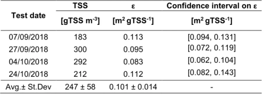
132
The light extinction coefficient inside the pond was estimated from four dedicated tests performed with an
133
immerged PAR probe (see Supplementary Information SI.1.1).
134
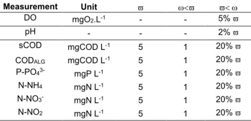
Standard deviations for on-line probes are computed using the probe variation coefficient (see Table SI.2.1).
135
The variation coefficients for off-line measurements represented on the graphs are given in Table SI.2.1, in
136
line with measurement accuracy and triplicate measurements.
137
138
2.2. Numerical tools
139
AQUASIM was used as numerical platform (Reichert, 1994). The HRABP was modelled as a completely
140
mixed reactor compartment. Raceways mixed by paddle wheels are generally considered to be perfectly
141
mixed (Solimeno et al., 2017). This hypothesis was validated by experimental measurements for the raceway
142
used in this study (Hreiz et al., 2014) .
143
The bioprocesses dynamics is described by means of the Petersen stoichiometric and kinetic matrix,
144
following the ASMs notation and structure, while the chemical processes are described as equilibrium
145
processes (algebraic equation system, see SI.6.1). The model was designed to guaranty the elemental
146
conservation of C, N, P, H, O and COD through the continuity check, that was carried out using the
147
stoichiometric and the composition matrix (see Tables SI.3.1, SI.3.2 and SI.3.3).
6
The ordinary differential equations (biological and transfer rates) and the algebraic equations (chemical
149
equilibria) are numerically integrated according to the DASSL algorithm (Petzold, 1982) implemented in
150
AQUASIM.151
152
2.2.1. Scenario analysis153
In this scenario analysis the idea is to represent the typical meteorological patterns characterizing each
154
season. Specifically, the weather was represented for each season (spring, summer, autumn and winter) by
155
a typical daily pattern for temperature, light and evaporation rate (see Figure 1). Four meteorological
156
scenarios were thus computed from local meteorological data by averaging hourly values (see Section 2.1).
157
Constant influent characteristics were assumed (as in Table 1). These realistic scenarios were used as a
158
basis to estimate the average fluxes and relevant quantities along each season. In this way, a typical daily
159
pattern was defined (Figure 1) and extended to run simulations under the established periodic regime. For
160
each season, two scenarios for the gas transfer rate were considered, representing two extreme solutions for
161
mixing the process.
162
The existing Algae-Bacteria models do not consider the contributions of rain and evaporation rates, even if
163
these two phenomena can significantly affect the hydraulic balance of the raceway (Bechet et al., 2018;
164
Pizzera et al., 2019). Indeed, the hydraulic loads are strongly affected by the meteorology, causing
165
considerable dilution or concentration of soluble and particulate compounds inside the reactor, therefore
166
affecting bioprocess rates as well as light availability. The evaporative contribution was estimated according
167
to the Buckingham equation (Bechet et al., 2011). Long term simulations were then run under periodic
168
regime, until a steady periodic response was reached. Results are shown and discussed in section 5.2.
169
170
2.2.2. Sensitivity analysis
171
The sensitivity analysis was carried out with the available AQUASIM toolboxes (Reichert, 1994), using the
172
long-term dataset from the monitoring campaign.
173
The absolute-relative sensitivity function was chosen to facilitate the comparison among the effect of
174
different parameters on the same dynamic variable. In addition, a ranking of the absolute values of the
175
sensitivity functions was implemented. The sensitivity function was studied for each season, considering the
176
stationary periodic regime.
177
178
7
179
Figure 1. Typical daily pattern of temperature, irradiance and evaporation rates according to the season
180
181
2.2.3. Parameters identification
182
First, simulations were run choosing model parameter values inside the ranges reported in similar works in
183
literature (see Table SI.8.1). A pre-calibration was first made by expert adjustment of these parameters to get
184
an overall coherent simulated dynamics over the full period. These parameter values where then taken as
185
initial conditions for the automatic fine-tuning parameter identification algorithm performed on the targeted
186
sub-set of parameters obtained from the sensitivity analysis.
187
The identification toolbox of AQUASIM was used which minimizes the sum of square errors between
188
simulated and experimental data weighted by standard deviations (Reichert, 1994):
189
χ2 p = ym,i-ys,i p σm,i 2 n i=1 (1)190
Where n is the number of measurements, ym,i and ys,i are the experimental and simulated variables
191
respectively, σm,i the deviation standard of experimental measurements and p is the parameter to be
192
determined to minimize the difference among experimental measurements and model predictions.
193
The simplex method was used to find a first set of optimized solutions, while the secant method was applied
194
to further reduce the prediction error (Reichert, 1994).
195
Since the current parameter values in the literature account for situations in spring or summer (or indoor at
196
warmer temperature), the calibration strategy had to counterbalance this inherent model ability to better
197
represent the warmest seasons. Indeed, the default parameter values are taken from algae-bacteria models
198
typically calibrated on a short-term period, under spring-summer or indoor conditions, resulting in limited
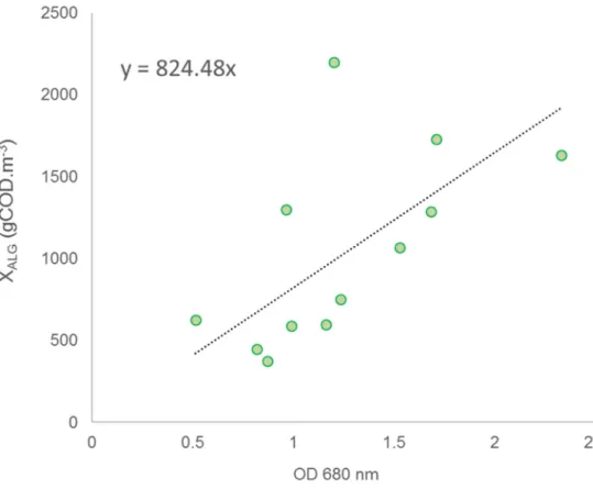
199
applicability range of the model. Two calibration periods were thus chosen in autumn and winter
(02-200
21/10/2018 and 01-10/01/2019) in order to cover a wider range of temperatures and weather conditions. No
8
additional calibration periods were considered to avoid a further reduction of the data for the validation
202
phase.
203
Since a correct prediction of pH and O2 is crucial to precisely predict the overall system dynamics, and since
204
these signals are directly or indirectly affected by all relevant biochemical and physical/chemical processes,
205
the online pH and O2 measurements were used as first target in the parameter estimation to get an upgraded
206
set of parameters. The information richness of this fluctuating signals revealed to be very beneficial for an
207
accurate calibration of ammonium, nitrite, nitrate, COD, optical density and TSS predictions. Expert
208
adjustment from the previous parameter set was then carried out to further improve the fit of the off-line
209
measurements. The procedure was repeated iteratively until a good fit was obtained for the calibration
210
period. A unique set of parameters was finally obtained and considered to simulate the experimental
211
campaign covering all seasons. The parameter uncertainty was derived from the Fisher information matrix,
212
as described in SI.9. The prediction error was derived from the parameter uncertainty and from the sensitivity
213
functions, as detailed in in SI.10.
214
Model validity was then assessed using the data of the monitoring campaign which were not used during
215
calibration (i.e. data from 414 days, out of 443 days).
216
217
2.2.4. Quality of fit
218
Model prediction performances were evaluated through the modified Theil’s Inequality Coefficient, TIC,
219
(Decostere at al., 2016) and the modified Mean Absolute Relative Error, MARE, (Hauduc et al., 2015) as
220
reported in Eq. 2 and 3:
221
TIC= ∑ satσ (ys,i,ym,i) i 2 ∑ yi s,i 2 + ∑ yi m,i 2 (2) MARE = 1 n ∙|satσ(ym,i,ys,i)|
ym,i+φ
n
i=1
(3)
Where the function sat (ys,i,ym,i is zero when both ym,i and ys,i are lower than the associated measurement
222
standard deviation (accepted as perfect fit situation), and otherwise: sat (ys,i,ym,i y, y ,. The small
223
correction factor φ (taken as 0.1) is applied to avoid division by zero.
224
Both criteria quantify the difference between model predictions and experimental values and normalize them
225
according to the magnitude of the considered variable. For both criteria, the closer the value to zero, the
9
better the model performance. The TIC and MARE criteria were computed for the measured variables on the
227
overall validation period (excluding the dataset used for calibration) and separately for each season.
228
229
3. ALBA model description
230
3.1. Biological model
231
The ALBA model includes 19 biological processes involving 17 state variables, classified as shown in Table
232
2. Reaction stoichiometry and rates are inspired by standard modelling works. However, some simplifications
233
were adopted to limit the complexity of this multiscale dynamic system, the main ones being listed hereafter.
234
First, the soluble organic biodegradable matter (SS) was assumed to be consumed only by heterotrophic
235
bacteria, even though most of the microalgae can grow heterotrophically or mixotrophically, at least for some
236
simple and easily biodegradable carbon sources such as glucose or acetate (Turon et al., 2015). However,
237
more complex carbon sources can be typically found in wastewaters (e.g. municipal and industrial waste
238
streams, digestate) and algae are generally not able to use them for their metabolism, or just a small fraction
239
of the algal population may be equipped with the suitable enzymes. For this reason, in the ALBA model it
240
was assumed that the algal growth is only autotrophic. In addition, the heterotrophic/mixotrophic algal
241
metabolism is still not well characterized for outdoor and non-axenic conditions, making the calibration of key
242
parameters more challenging (e.g. specific growth rate, affinity to specific substrate, dependence on
243
environmental conditions, etc.).
244
Predation was not explicitly considered and it was integrated into the mortality term. Organic matter and
245
nutrient storage processes as intermediate step for biomass growth were not considered. Hydrolysis
246
processes, both for urea and slowly biodegradable COD, are assumed to be performed by heterotrophic
247
bacteria only. Consistently with experimental records for real and synthetic wastewaters, micronutrients were
248
assumed to be abundant and never limiting.
249
In summary, the following processes have been considered:
250
ρ1 – Algae phototrophic growth using NH4+ as nitrogen source. Inorganic carbon is used under the form of
251
CO2 and HCO3- and oxygen is produced, while soluble phosphorous and ammonium are uptaken.
252
ρ2 – Algae phototrophic growth, using NO3- as nitrogen source. This is not the favoured way for growing,
253
since it requires more energy. Therefore, it takes place when ammonium is limiting. Main products are
254
biomass and oxygen, while inorganic carbon, nitrate, and phosphorus are consumed.
10
ρ3 – Algae respiration. This process accounts for biomass loss, with oxygen consumption and production of256
CO2. Typically, in ASM models, there is only one process to account for either endogenous respiration or
257
decay. Here, these two processes are distinguished, assuming oxygen consumption occurs only during
258
respiration.
259
ρ4 – Microalgae decay, without oxygen consumption, releasing nutrients and organic matter, in line with
260
other algae-bacteria models (RWQM1 and BioAlgae2).
261
ρ5 – Aerobic growth of heterotrophic bacteria using NH4+ as nitrogen source. This is the preferential way for
262
growth under aerobic conditions. Growth also requires a source of carbon and energy (soluble organic
263
matter), phosphorus and oxygen and results in CO2 production.
264
ρ6 – Aerobic growth of heterotrophic bacteria on NO3- as nitrogen source. This is a secondary way for growth
265
of heterotrophs under aerobic conditions when ammonium is limiting, but it requires more energy leading to a
266
lower growth yield.
267
ρ7 – Aerobic respiration of heterotrophic bacteria (same assumptions as for algae).
268
ρ8 – Anoxic growth of heterotrophic bacteria using NO3- as electron acceptor. This reaction occurs when
269
oxygen is not available.
270
ρ9 – Anoxic growth of heterotrophic bacteria on NO2- as election acceptor. As for process ρ8, this reaction
271
occurs only when oxygen concentration becomes too low.
272
ρ10 – Anoxic respiration of heterotrophic bacteria, using NO2- and NO3- instead of O2 as electron acceptor. It
273
takes place only for low concentrations of Dissolved Oxygen (DO).
274
ρ11 – Hydrolysis of slowly biodegradable organic matter. This process is performed by heterotrophic bacteria
275
through an enzymatic reaction, where complex organic substances are transformed into readily assimilable
276
forms and a fraction of the hydrolysed organic matter is transformed into inert soluble form.
277
ρ12 – Hydrolysis of urea. This is an enzymatic reaction performed by heterotrophs, without oxygen
278
consumption, transforming urea into ammoniacal nitrogen and CO2.
279
ρ13 – Decay of heterotrophic bacteria, modelled similarly to algae decay.
280
ρ14 – Aerobic growth of AOB. In line with the approach followed by Iacopozzi et al. (2007) and in the RWQM1
281
model, the two-step nitrification process has been implemented to reproduce the accumulation of nitrite
282
observed experimentally. It involves oxygen consumption for ammonium oxidation into nitrite, from which the
11
energy necessary for AOB growth is derived. Inorganic carbon is used as carbon source and phosphorus is
284
uptaken.
285
ρ15 – Aerobic respiration of AOB, similarly to algae respiration.
286
ρ16 – Decay of AOB, modelled similarly to algae decay.
287
ρ17 – Aerobic growth of NOB. Oxygen is used for nitrite oxidation to nitrate to get the energy for biomass
288
production. Inorganic carbon is used as carbon source and phosphorus is uptaken.
289
ρ18 – Aerobic respiration of NOB, similarly to algae respiration.
290
ρ
19–
Decay of NOB,
modelled similarly to algae decay.291
Bioprocess stoichiometry and kinetics are described in the following Sections 3.1.1 and 3.1.2.
292
293
3.1.1. Bioprocess stoichiometry
294
One of the originalities of the ALBA model is to describe the phototrophic growth of microalgae considering
295
the main nutrients and metabolites (CO2, HCO3-, NH4+, PO43-, O2) affecting their kinetics. The algae biomass
296
elementary composition is taken from Grobbelaar (2004), accounting for C, H, O, N, P and neglecting
297
micronutrients (e.g.: Fe, Mg). The source of inorganic nitrogen is assumed to be ammonium or nitrate.
298
Reaction stoichiometry for algae growth on ammonium and nitrate is reported in Supplementary information,
299
Table SI.3.1. It is worth emphasising that the ALBA model accounts for P assimilation while existing models
300
do rarely consider P in the biomass raw formula. Moreover, the design of the model guarantees the
301
elemental conservation of C, N, P, H, O and the COD conservation.
302
All the stoichiometric parameter values and their expressions as implemented in the stoichiometric matrix,
303
can be found in Supp. Info (Table SI.3.2 and SI.3.3).
304
305
12
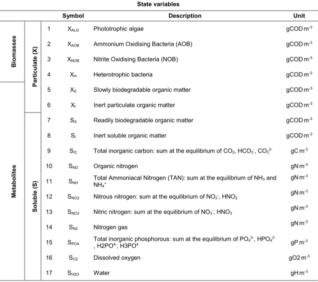
Table 2. State variables included in the ALBA model.306
State variables
Symbol Description Unit
B io m a s s e s P a rt ic u la te ( X )
1 XALG Phototrophic algae gCODm-3
2 XAOB Ammonium Oxidising Bacteria (AOB) gCODm-3
3 XNOB Nitrite Oxidising Bacteria (NOB) gCODm-3
4 XH Heterotrophic bacteria gCODm-3
M e ta b o li te s
5 XS Slowly biodegradable organic matter gCODm-3
6 XI Inert particulate organic matter gCODm-3
S o lu b le ( S )
7 SS Readily biodegradable organic matter gCODm-3
8 SI Inert soluble organic matter gCODm-3
9 SIC Total inorganic carbon: sum at the equilibrium of CO2, HCO3-, CO32- gCm-3
10 SND Organic nitrogen gNm-3
11 SNH Total Ammoniacal Nitrogen (TAN): sum at the equilibrium of NH3 and
NH4+
gNm-3
12 SNO2 Nitrous nitrogen: sum at the equilibrium of NO2-, HNO2
gNm-3
13 SNO3 Nitric nitrogen: sum at the equilibrium of NO3-, HNO3
gNm-3
14 SN2 Nitrogen gas
gNm-3
15 SPO4 Total inorganic phosphorous: sum at the equilibrium of PO4
3-, HPO 4
2-, H2PO4-, H3PO4 gPm-3
16 SO2 Dissolved oxygen gO2m-3
17 SH2O Water gHm-3
307
3.1.2 Bioprocess kinetics
308
The process rates are described in Table 3, (ρi, where i is the process number, as listed before). Every rate
309
accounts for the effect of nutrient concentration (limitation or inhibition) and of environmental conditions
310
(light, temperature, pH) through the product of Monod terms and dedicated relationships (fI, fT, fpH, fO2,G,
311
fO2,D). A special focus on these mathematical expressions is reported below.
312
313
13
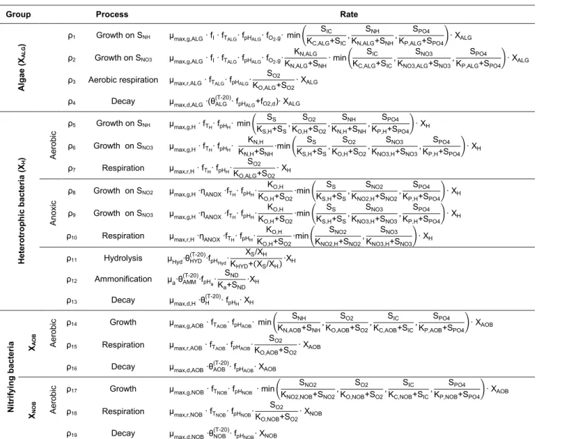
Table 3. Biological process rates in the ALBA model.314
Group Process Rate
A lg a e ( XA L G )
ρ1 Growth on SNH μmax,g,ALG ∙ fI ∙ fTALG∙ fpHALG∙ fO2,g∙ min
SIC KC,ALG+SIC , SNH KN,ALG+SNH , SPO4 KP,ALG+SPO4 ∙ XALG
ρ2 Growth on SNO3 μmax,g,ALG ∙ fI ∙ fTALG∙ fpHALG∙ fO2,g∙
KN,ALG KN,ALG+SNH ∙ min SIC KC,ALG+SIC , SNO3 KNO3,ALG+SNO3 , SPO4 KP,ALG+SPO4 ∙ XALG
ρ3 Aerobic respiration μmax,r,ALG ∙ fTALG∙ fpHALG∙
SO2
KO,ALG+SO2∙ XALG
ρ4 Decay μmax,d,ALG ∙(θALG
(T-20)
∙ fpHALG+fO2,d)∙ XALG
H e te ro tr o p h ic b a c te ri a ( XH ) Ae ro b ic
ρ5 Growth on SNH μmax,g,H ∙ fTH∙ fpHH∙ min
SS KS,H+SS , SO2 KO,H+SO2 , SNH KN,H+SNH , SPO4 KP,H+SPO4 ∙ XH
ρ6 Growth on SNO3 μmax,g,H ∙ fTH∙ fpHH∙
KN,H KN,H+SNH∙min SS KS,H+SS, SO2 KO,H+SO2, SNO3 KNO3,H+SNO3, SPO4 KP,H+SPO4 ∙ XH ρ7 Respiration μmax,r,H ∙ fTH∙ fpHH∙ SO2 KO,ALG+SO2 ∙ XH A n o x ic
ρ8 Growth on SNO2 μmax,g,H ∙ηANOX ∙fTH∙ fpHH∙
KO,H KO,H+SO2 ∙min SS KS,H+SS , SNO2 KNO2,H+SNO2 , SPO4 KP,H+SPO4 ∙ XH
ρ9 Growth on SNO3 μmax,g,H ∙ηANOX ∙fTH∙ fpHH∙
KO,H KO,H+SO2 ∙min SS KS,H+SS , SNO3 KNO3,H+SNO3 , SPO4 KP,H+SPO4 ∙ XH
ρ10 Respiration μmax,r,H ∙ηANOX ∙fTH∙ fpHH∙
KO,H KO,H+SO2 ∙min SNO2 KNO2,H+SNO2 , SNO3 KNO3,H+SNO3 ∙ XH
ρ11 Hydrolysis μHyd∙θHYD (T-20)∙f pHHyd∙ XS/XH KHYD+ XS/XH ∙XH ρ12 Ammonification μa∙θAMM (T-20) ∙fpHa∙ SND Ka+SND ∙XH ρ13 Decay μmax,d,H ∙θH (T-20)∙ f pHH∙ XH N it ri fy in g b a c te ri a X A O B A e ro b
ic ρ14 Growth μmax,g,AOB ∙ fTAOB∙ fpHAOB∙ min
SNH KN,AOB+SNH, SO2 KO,AOB+SO2, SIC KC,AOB+SIC, SPO4
KP,AOB+SPO4 ∙ XAOB
ρ15 Respiration μmax,r,AOB ∙ fTAOB∙ fpHAOB∙
SO2
KO,AOB+SO2∙ XAOB
ρ16 Decay μmax,d,AOB ∙θAOB
(T-20) ∙ fpHAOB∙ XAOB XN O B A e ro b
ic ρ17 Growth μmax,g,NOB ∙ fTNOB∙ fpHNOB ∙ min
SNO2 KNO2,NOB+SNO2 , SO2 KO,NOB+SO2 , SIC KC,NOB+SIC , SPO4 KP,NOB+SPO4 ∙ XAOB
ρ18 Respiration μmax,r,NOB ∙ fTNOB∙ fpHNOB∙
SO2
KO,NOB+SO2
∙ XNOB
ρ19 Decay μmax,d,NOB ∙θNOB(T-20)∙ fpHNOB∙ XNOB
* SIC in the Monod terms incudes the inorganic carbon coming from CO2 and HCO3-, without accounting for the contribution given by CO32- . The concentration of CO2 and HCO3- is estimated using the pH
315
sub-model, as shown in Appendix B, Equation 2B and 3B.
14
Nutrients
317
The ASMs models generally adopt a Monod type function to describe nutrient dependence in biological
318
kinetics requiring two parameters (μmax, KS). Often, nutrient dependence has been modelled in literature by
319
multiplying the different limiting functions. The use of these conventional multiplicative Monod terms is well
320
known to overestimate the growth limitation in presence of multiple limiting nutrients, therefore the Liebeg’s
321
minimum law was preferred to be closer to reality (Bougaran et al. 2010, Dolman and Wiedner 2015),
322
especially when simulating sub-optimal conditions in terms of substrate availability for the different
323
biomasses. The minimum law assumes (Lee et al., 2015)that the most limiting nutrient drives the growth
324
kinetics.
325
This approach was applied for the limiting substrates only but not for light, temperature or pH (Equation 4). In
326
modelling the effect of nutrient inhibition on biomass growth (see processes ρ2, ρ6, ρ8, ρ9, ρ10 in Table 3), a
327
hyperbolic-inhibition function was chosen, in line with the approach used in both ASMs and ADM1.
328
The general expression describing the biological process rates structure writes:
329
330
ρi,growth =μmax,i∙fT,i∙fpH,i∙fI∙
Kn Kn+Sn ∙min Sj Kj+Sj j ∙XBM,i (4)
331
where μmax is the maximum specific growth rate [d-1]; fT, fpH and fI are the functions describing temperature,
332
pH and light dependence, respectively, detailed in the following paragraphs; Kn is the inhibition constant for
333
the inhibiting substrate Sn, Kj is the half-saturation constant for the limiting substrate Sj and XBM,i is the
334
associated biomass. The specific expressions of each process are shown in Table 3.
335
336
337
Light
338
Light is a crucial factor for algae growth, driving a large fraction of the energy and carbon fluxes in the
339
system. Describing its effect on photosynthesis in a turbid system is challenging since it is affected by many
340
different factors and it is species dependent (Martinez et al. 2018). As stated before, light penetration in the
341
HRABP was estimated through the Lambert-Beer law (see Equation SI.1.1) and the light extinction
342
coefficient (ε) was experimentally determined, as reported in supplementary information (SI 1).
343
The light dependence of algal growth was described by a Haldane-type function (Equation 5), choosing the
344
parametrization proposed by Bernard and Remond (2012).
15
fI = μMAX I I+μMAX α I IOPT-1 2 (5)346
This function includes three parameters: maximum specific growth rate (μmax), optimal light for growth (IOPT)
347
and the initial slope of light response curve (α). The values chosen for IOPT and α are close to those reported
348
in similar works (Martinez et al., 2018; Rossi et al., 2020), while μMAX was calibrated (see section 2.2).
349
The function fI was integrated along the liquid depth inside the raceway (i.e. the light path), to compute the
350
average algae growth rate as a function of the available light intensity at each depth, according to the
351
approached followed by Martinez et al. (2018).
352
353
Temperature
354
Temperature deeply affects biological process rates, and this influence must definitely be considered for
355
outdoor systems. In this study, temperature fluctuates within large ranges along the campaign period,
356
through daily oscillations and seasonal changes.
357
The model chosen for simulating the temperature dependence of growth and respiration rates, both for algae
358
and bacteria, is the CTMI (Cardinal Temperature Model with Inflection) proposed by Rosso et al. (1993),
359
shown in Equation 6. This function has been shown to efficiently describe biomass growth, especially at high
360
temperatures. It requires three parameters (the cardinal temperatures: TMAX, TOPT, TMIN), which define the
361
optimal working range for each species.
362
An Arrhenius function, requiring only one parameter (θ in Equation 7), was implemented for modelling the
363
decay rate dependence on temperature for both algae and bacteria. With this function, the decay rate
364
increases with temperature. Nominal and calibrated cardinal temperature values are shown later on in
365
Table SI.8.1.366
fT= ⎩ ⎪ ⎨ ⎪ ⎧ 0 T-TMAX ∙ T-TMIN 2TOPT-TMIN ∙ TOPT-TMIN ∙ T-TOPT - TOPT-TMAX ∙ TOPT+TMIN-2T
0 T<Tmin Tmin≤T≤Tmax T>Tmax (6) fT= μDecay(T) μDecay(20°C) = θ (T-20) (7)
367
pH
368
16
The pH strongly influences system dynamics, since it directly affects the speciation of soluble compounds
369
(SIC, SNH, SNO2, SNO3, SPO4) and their availability.
370
The pH of the raceway was not controlled, so that the system exhibited large daily pH fluctuations (up to 10.5
371
during day and down to 7 during night). The pH dependence was modelled using the CPM (Cardinal pH
372
Model, without inflection, Equation 8) function proposed by Rosso et al. (1995).
373
The CPM requires three parameters (the cardinal pH: pHMAX, pHOPT, pHMIN), defining the growing range for
374
each biomass.375
fpH= ⎩ ⎪ ⎨ ⎪ ⎧ 0 pH-pHMIN ∙ pH-pHMAXpH-pHMIN ∙ pH-pHMAX - pH-pHOPT 2
0 pH < pHMIN pHMIN ≤ pH ≤ pHMAX pH > pHMAX (8)
376
Nominal and calibrated cardinal pH values are reported in Table SI.8.1.
377
378
Oxygen
379
High dissolved oxygen concentrations can negatively affect the photosynthetic activity of phototrophic
380
microorganisms (Peng et al., 2013). The reduction of photosynthetic activity at high O2 concentrations can be
381
described with an inhibition Hill-type model (Equation 9) in the growth rate (Di Veroli et al., 2015):
382
fDO,G = kDO n SO2n +kDOn (9)where kDO is the inhibition parameter of the model and n is the dimensionless Hill coefficient [-]. Oxygen is
383
the substrate of algae respiration and its limiting effect is classically represented with a Monod-type function
384
(see Table 3).
385
The effect of high oxygen concentration on algal mortality was represented with a Hill-type model (Equation
386
10), as reported in Table 3. It represents the increase in the decay rate above a certain oxygen concentration
387
(kDO):388
fDO,D= SO2n SO2 n +kDO n (10)The parameters values were taken from literature (Rossi et al., 2020).
389
390
3.2. Chemical and physical sub-models
391
3.2.1. pH sub-model
17
Modelling inorganic carbon and pH dynamics (together with oxygen) is the cornerstone of the algae-bacteria
393
interactions. The pH evolution results from the dynamical balance between the chemical, physical and
394
biological process interactions. The pH model is based on dissociation equilibria and mass balances of acids
395
and bases, as in the ADM1 (Anaerobic Digestion Model n.1, Batstone et al., 2002) and on the charge
396
balance, through which it is possible to determine the concentration of hydrogen ions, consequently the pH
397
of the system. Explicit equations and dissociation constants, together with their temperature dependency are
398
provided in Sup. Info (Table SI.5.1). Note that the pH sub-model considers much more chemical species
399
than the simplified pH models involved in the other algae-bacteria models, being therefore more appropriate
400
for simulating case studies where the pH is not controlled and where extreme values can be reached.
401
The variable ΔCAT,AN is the difference between cationic and anionic species which do not enter explicitly in the
402
charge balance. Since none of the processes acts on ΔCAT,AN, its dynamics simply depends on the incoming
403
buffering capacity.
404
405
3.2.2. Gas – liquid transfer
406
The open pond has a large surface exchanging with the atmosphere, consequently gas-liquid mass transfer
407
(O2, CO2 stripping/dissolution, NH3 stripping) must be implemented. The general expression for the mass
408
transfer kinetics can be described through the Fick's law (Equation 11):
409
Qj=kLaj Sj,SAT-Sj (11)
Where Qj is the transfer rate for the gas Sj [g m-3 d-1], kLa is the global mass transfer coefficient [d-1], Sj is the
410
gas concentration [g m-3] and Sj,SAT is the gas concentration at saturation conditions [g m-3]. Sj,SAT is
411
expressed through the Henry’s law (Equation 12):
412
Sj,SAT=HSj∙pSj (12)
where HSj is the Henry constant for the gas Sj [g m-3 atm-1] and pSj is the gas partial pressure at the interface
413
[atm]. The different mass transfer coefficients and their temperature dependence are described in SI.7.
414
415
3.2.3. Connecting simulated variable with measured quantities
416
417
Experimental measurements of COD and TSS were compared with the simulated variables computed as
418
follows: TSS= [(XALG/1.57)+(XI+XS+XAOB+XNOB+XH)/1.46] and CODs=SS+SI. The coefficient 1.57 gCOD
419
gBMALG-1 and 1.46 gCOD gBMBAC-1 are the conversion factors computed for algae and bacteria respectively
18
using the stoichiometry described in SI. 4. Algal COD was estimated from absorption measurements using
421
the following correlation: XALG,meas=824.48*OD680 (See SI.1.2).
422
423
4. Results
424
4.1. Sensitivity analysis and parameter estimation
425
426
The large number of parameters involved in the ALBA model (135 in total, including the parameters
427
characterizing chemical constants and their temperature dependence) is a major challenge for its calibration.
428
A sensitivity analysis was thus needed to identify a subset of parameters among the most sensitive ones,
429
which are then identified by the calibration procedure. Results are reported in Supp. Info Table SI.8.1. It is
430
worth noting that all the parameters that were classified as the most sensitive ones and therefore included
431
into the calibration procedure directly or indirectly impact the pH and dissolved oxygen dynamics, making
432
these easily measurable on-line signals of great relevance in parameters identification.
433
Kinetic parameters related to microalgae and nitrifying bacteria were among the most sensitive ones. In
434
particular, the maximum specific growth rate of AOB and NOB had a substantial effect on nitrogen forms, DO
435
and pH dynamics.
436
The algal biomass concentration is highly influenced by parameters related to the photosynthesis-irradiance
437
curve, similarly to previous findings (Rada-Ariza, 2018). Indeed, both the light extinction coefficient, the initial
438
slope of the light response curve, and the optimal irradiance value strongly affect the predicted values of
439
microalgae concentration, DO and pH.
440
The mass-transfer coefficient (kLa) turned out to govern all the gas-liquid exchanges (i.e. NH3, CO2 and O2),
441
also influencing pH, and consequently the biological process rates and dissociation equilibria. It was
442
therefore calibrated, with the resulting value falling in the literature range (Mendoza et al., 2013; Caia et al.,
443
2018).
444
The cardinal temperatures and pH values in the Rosso functions were also found to be among the most
445
sensitive parameters. For algae, the calibrated TMAX threshold is close to the nominal value, while lower
446
values were obtained for TOPT and TMIN. Regarding pH, calibrated thresholds are close to those proposed by
447
Ippoliti et al. (2016). The calibrated pHMIN was also experimentally observed in activity tests performed on
448
algae-bacteria samples from a similar pilot-scale HRABP treating the liquid fraction of digestate from a waste
449
sludge full scale digester (Rossi et al., 2020). The cardinal values for AOB and NOB are slightly different
450
from those previously suggested for conventional activated sludge plant, where the working pH range is
451
typically around neutrality.
19
The coefficients for temperature dependence for organic carbon and nitrogen hydrolysis were found to
453
remarkably influence simulation results. This is due to the key role played by temperature on these
454
processes, which is especially relevant in systems where the availability of ammoniacal nitrogen and/or
455
readily biodegradable organic compounds strictly depends on the hydrolysis efficiency. COD fractionation
456
and alkalinity had also a strong impact on model results, but they can be easily measured.
457
458
4.2. Model performances on relevant variables
459
4.2.1. Nycthemeral dynamics
460
461
Model performances in reproducing daily dynamics for dissolved oxygen and pH are discussed in this
462
section. For each variable, three days were selected for each season and reported in Figure 2. The selected
463
days in autumn belong to the calibration period, to illustrate the very good model fit obtained (Figure2b).
464
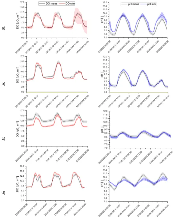
The ALBA model proved to accurately capture nycthemeral dynamics reflected in the on-line signals, as
465
shown in Figure 2. It is worth noting that the oxygen dynamics in response to light results in more complex
466
profiles during cloudy days (Figure 2b and Figure 2d). During the night, the simulated oxygen is stable or
467
slightly increasing, depending on the balance between higher oxygen solubility due to lower temperatures
468
and biological consumption rates. The model confidence interval for the maximum oxygen level slightly
469
overestimates the measured oxygen mostly in spring (Figure 2d) and during the central part of the day. In
470
summer, oxygen production during the hours of highest irradiance is underestimated probably because of
471
light inhibition.
472
During winter, the model is still efficient in predicting the dissolved oxygen dynamics, but the simulated
473
values underestimate the real ones by about 3 mg L-1 (Figure 2c) suggesting that the set of calibrated
474
parameters are less effective in capturing the winter behaviour. It must be made clear that all the simulated
475
data were obtained with the same parameter set.
476
The pH dynamics is correctly captured in almost all the seasons. During spring 2019, the raceway reached
477
the highest pH values and the corresponding predictions are less accurate. Under those high pH values,
478
other phenomena could take place, such as salts precipitation which are not included in the ALBA model but
479
that may affect the pH value.
480
481
20
a)b)
c)
d)
Figure 2. Nycthemeral dynamics for DO and pH. Comparison of typical trends for measured (black), simulated
482
DO (red) and simulated pH values (blue) during four seasons: summer (a), autumn (b), winter (c) and spring (d).
483
Grey shaded areas represent the standard deviation of each experimental measurement. Red and blue shaded
484
areas, for simulated DO and pH respectively, represent the 95% confidence intervals of model predictions.
485
Yellow bars under the time-axis indicates that the data were used for parameter calibration.
486
487
488
4.2.2. Long-term dynamics
489
490
Once calibrated, the ALBA model was validated over a long-term experimental data set. Hereafter, its
491
performances along with its ability to follow long term patterns, over a one-year period are discussed. It must
492
be stressed that all the simulated long-term data shown in Figure 3 were obtained with the same parameter
493
set used in the previously described nycthemeral pH and DO variation along the seasons. Satisfactory
494
model performances can be observed for all data series including nitrogen compounds, biomass
21
concentration, COD, pH and DO values. In addition, the model performances were evaluated with the two
496
model performance indices, TIC and MARE, on the entire period and separately for the different seasons
497
(Table 4).
498
Accurately simulating the nitrogen compounds dynamics is challenging, since their concentrations are
499
affected by almost all the processes taking place in the reactor. The best predictions for nitrogen compounds
500
are obtained in spring and summer, while in autumn and winter simulations are less accurate (Figure 3a and
501
3b and Table 4). At the beginning of august 2018, a switch from partial to total nitrification was observed, and
502
appropriately simulated, as shown by the decrease in nitrite concomitant with the increase in nitrate
503
concentration (Figure 3b). It is worth remarking that the model prediction uncertainty becomes high around
504
the switching time. It probably means that this switching time is highly sensitive to the parameter values and
505
the initial conditions for biomass concentrations. Total nitrification becomes less efficient in autumn and
506
winter, because of the decreasing temperature. This leads to a decrease in NOx concentrations and an
507
increase in the ammonium concentration, also affected by the reduction in algae contribution to ammonium
508
removal by assimilation. During winter, urea hydrolysis slows down remarkably, thus reducing the
509
ammoniacal nitrogen availability in the system. Models for urea hydrolysis and their dependence on
510
environmental parameters are missing in the literature. Therefore, the lower accuracy of the model during
511
winter can be also attributed to a sub-optimal description of this poorly known process. It is worth noting that
512
parameters related to denitrification and ammonia stripping were assumed from literature (see Table SI.5.1),
513
therefore an insight in the dynamics of these processes would possibly improve the predictions of the
514
nitrogen compounds.
515
The simulated algae biomass concentration, expressed in COD, is compared with the measurements derived
516
from optical density at 680 nm in Figure 3c. The predicted algae concentration responded markedly to
517
seasonal changes and fit well the measurements.
518
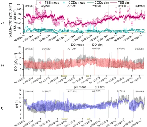
Model performances were assessed for TSS and soluble COD along all the year (Figure 3d).
519
The low values of both the total TIC and the MARE criteria for TSS (0.13 and 0.26 respectively) highlight the
520
model accuracy. The seasonal model predictions are slightly less accurate in spring and winter. This is
521
possibly due to the influence of the start-up period (spring) which is affected by the selection of the initial
522
conditions.
523
The soluble COD dynamics is generally well predicted by the model (Figure 3d). Spring and autumn 2018
524
are the most critical seasons in terms of goodness of fit. The same comments already reported as for TSS
525
can be applied in the case of COD as well.
22
The sensitivity analysis revealed how pH and dissolved oxygen dynamics play a central role by affecting the
527
overall balance among microbial populations. Thus, a correct prediction of these variables is of the utmost
528
importance for the accurate prediction of the overall system behaviour. Indeed, a generally good agreement
529
between model predictions and experimental values was obtained for both dissolved oxygen and pH, as
530
show in Figure 3e and Figure 3f. This is confirmed from the total TIC (0.03 and 0.11 for pH and DO,
531
respectively) and MARE values (0.05 and 0.18 for pH and DO respectively). Looking at pH seasonal trends,
532
the model accuracy is satisfactory in all the periods. Also, for the dissolved oxygen, the overall model
533
efficiency criteria were satisfactory met, with a lower accuracy during winter.
534
It must be stressed that the MARE coefficients for nitrogen compounds and soluble COD are higher than the
535
ones reported for the other measurements (TSS, DO, pH), but these fit criteria are known to amplify small
536
model misfit when values are close to zero (Hauduc et al. 2015).
537
The model efficiently predicts most variable trends, demonstrating a sound prediction capability.
538
A better model fit could of course be obtained if a season-dependent set of parameters is chosen.
539
540
a)
b)
23
d)e)
f)
Figure 3. Long-term evolution of measured and simulated variables: ammonium (a), nitrite and nitrate (b),
541
simulated algal biomass and measured optical density (c), Soluble organic compounds and Total Suspended
542
Solids concentrations (d), dissolved oxygen (e), and pH (f). Error bars on experimental measurements represent
543
their standard deviation. Shaded areas on model predictions represent the related 95% confidence intervals.
544
Yellow bars under the time-axis indicates the calibration period. Coloured vertical bars in pH and DO graphs
545
indicate the short-term dynamics represented on Figure 2.
546
547
548
Table 4. Model efficiency criteria evaluated for different variables in different seasonal conditions.
549
Theil’s Inequality Coefficient - TIC
Total Spring Summer Autumn Winter
pH 0.03 0.03 0.04 0.03 0.02 O2 0.11 0.09 0.10 0.12 0.13 N-NH4+ 0.35 0.33 0.53 0.43 0.43 N-NO2- 0.18 0.26 0.16 0.67 0.69 N-NO3- 0.18 0.27 0.12 0.21 0.25 XALG 0.15 0.19 0.11 0.20 0.21 TSS 0.13 0.17 0.13 0.13 0.14 CODs 0.25 0.31 0.18 0.31 0.24
Mean Absolute Relative Error - MARE
pH 0.05 0.05 0.07 0.04 0.03 O2 0.18 0.16 0.18 0.19 0.21 N-NH4+ 0.69 0.86 0.66 0.60 0.53 N-NO2- 0.52 0.63 0.42 0.76 0.66 N-NO3- 0.50 0.64 0.22 1.02 0.37 XALG 0.31 0.41 0.23 0.38 0.31 TSS 0.26 0.29 0.24 0.20 0.31 CODs 0.51 0.42 0.44 0.84 0.26
550
24
5. Discussion
551
5.1 Decisive modelling choices
552
553
Designing a model, especially for a complex outdoor biological process is the sum of many subtle and
554
strategic choices (Mairet and Bernard, 2019). We detail hereafter the most determinant modelling choices,
555
highlighting the main differences between ALBA and pre-existing algae-bacteria models.
556
Generally, nutrient limitation is computed as the product of all the functions affecting the process rates. This
557
modelling choice was followed by most of the other algae-bacteria models, as RWQM1, BioAlgae2 and the
558
Modified ASM3. However, multiplying limitation factors may lead to an undesired underestimation in
559
quantifying the real biological activity, in presence of several limiting nutrients. For this reason, the Liebig’s
560
law was chosen to more accurately represent multi limitation situations (see Equation 4 and Table 3), since it
561
describes that the most limiting nutrient drives the overall kinetics.
562
A similar strategy was adopted by the PHOBIA model, which however included the limiting and inhibiting
563
factors for nutrient and light dependence in the minimum function argument.
564
Only few algae-bacteria models considered a dedicated sub-model to describe the dynamic evolution of pH.
565
So far, the most detailed pH model was found in the RWQM1, considering chemical equilibria for ammonium,
566
bicarbonate, phosphates and calcium. It is worth pointing out that the DO and pH dynamics contained
567
enough information to strongly constrain the most influent model parameters in the identification process. A
568
correct prediction of DO and pH is therefore crucial to accurately simulate the overall system behaviour.
569
Temperature turns out to play a direct (on solubility) and indirect (on activities) role on the dynamics.
570
The specific choice for the functions representing the pH and oxygen impacts (also at high oxygen
571
concentration) is thus important. In particular, it turns out that a distinct set of cardinal temperature and pH
572
values is necessary to represent the dynamics of AOB and NOB.
573
Improvement in the pH model could still be made, accounting for the precipitation of several salts, especially
574
at high pH values.
575
Rainfall and evaporation in outdoor conditions can have strong impact on the hydraulic balance of the
576
raceway and must definitely be included in the modelling. Evaporation was relevant mostly in spring and
577
summer, accounting on average for up to 15 - 25% of the influent flowrate.
578
Finally, the powerful calibration strategy associated with the ALBA model is also an important ingredient in
579
the efficient model validation, from where the key role played by oxygen and pH dynamics clearly emerged.
580
The seasonal sensitivity analysis provided the most sensitive parameters in every meteorological condition