Enhancement of electric and magnetic wave fields at density gradients

HAL Id: hal-00317941

https://hal.archives-ouvertes.fr/hal-00317941

Submitted on 7 Mar 2006

HAL is a multi-disciplinary open access

archive for the deposit and dissemination of

sci-entific research documents, whether they are

pub-lished or not. The documents may come from

teaching and research institutions in France or

abroad, or from public or private research centers.

L’archive ouverte pluridisciplinaire HAL, est

destinée au dépôt et à la diffusion de documents

scientifiques de niveau recherche, publiés ou non,

émanant des établissements d’enseignement et de

recherche français ou étrangers, des laboratoires

publics ou privés.

Enhancement of electric and magnetic wave fields at

density gradients

A. Reiniusson, G. Stenberg, P. Norqvist, Anders I. Eriksson, K. Rönnmark

To cite this version:

A. Reiniusson, G. Stenberg, P. Norqvist, Anders I. Eriksson, K. Rönnmark. Enhancement of electric

and magnetic wave fields at density gradients. Annales Geophysicae, European Geosciences Union,

2006, 24 (1), pp.367-379. �hal-00317941�

SRef-ID: 1432-0576/ag/2006-24-367 © European Geosciences Union 2006

Annales

Geophysicae

Enhancement of electric and magnetic wave fields at density

gradients

A. Reiniusson1, G. Stenberg1,2, P. Norqvist1, A. I. Eriksson2, and K. R¨onnmark1

1_{Department of Physics, Ume˚a University, Ume˚a, Sweden} 2_{Swedish Institute of Space Physics, Uppsala, Sweden}

Received: 26 August 2005 – Accepted: 20 December 2005 – Published: 7 March 2006

Abstract. We use Freja satellite data to investigate irregular

small-scale density variations. The observations are made in the auroral region at about 1000–1700 km. The density vari-ations are a few percent, and the structures are found to be spatial down to a scale length of a few ion gyroradii. Irreg-ular density variations are often found in an environment of whistler mode/lower hybrid waves and we show that at the density gradients both the electric and magnetic wave fields are enhanced.

Keywords. Magnetospheric physics (Auroral phenomena)

– Space plasma physics (Wave-particle interactions; Waves and instabilities)

1 Introduction

Whistler mode and lower hybrid waves are frequently ob-served on auroral field lines. Sudden enhancements of the wave power in these modes are often associated with small-scale density variations. One common type of small-small-scale density structure was initially observed at altitudes below 1500 km (e.g. Fejer and Kelley, 1980; Sagalyn et al., 1974). These structures have scale lengths down to about the ion gyro radius and are referred to as spatial irregularities: the density profile varies irregularly and the density depletions are generally a few percent. Holmgren and Kintner (1990) use data from the Viking satellite to show the existence of such irregular static structures also at higher altitudes and lat-itudes. Other observations of irregular structures have been made by Temerin (1978), using S3-3 data, and by Delory et al. (1997), using Alaska ’93 sounding rocket data. De-lory et al. (1997) show that waves with very short wave-lengths can be found on small-scale density gradients, while waves between the structures have much longer wavelengths. Hence, they suggest that mode conversion occurs on the den-sity gradients.

Correspondence to: A. Reiniusson

(annie.reiniusson@space.umu.se)

Another well-known type of density depletion is the so-called Lower Hybrid Cavity (LHC) or Lower Hybrid Solitary Structure (LHSS). LHCs are elongated structures aligned with the background magnetic field observed both by rockets on low altitudes and by numerous satellites on altitudes up to 35 000 km (Tjulin et al., 2003; Schuck et al., 2003 and refer-ences therein). They are found to be spatial structures (e.g. Knudsen et al., 1998) with a Gaussian-shaped density profile perpendicular to the ambient magnetic field. The width of a typical cavity is a few ion gyroradii and the density depletion is a few percent up to several tens of percent. Previous studies using data from the Freja satellite show clear enhancements of the electric wave power on the density gradients of LHCs, while no increases in the magnetic wave power are reported (e.g. Høymork et al., 2000; Dovner et al., 1994; Eriksson et al., 1994). These observations are consistent with theoret-ical models that predict electrostatic or almost electrostatic waves to be trapped in the cavities (Schuck et al., 2003; Hall et al., 2004). However, recent rocket observations indicate that LHCs sometimes can be associated with electromagnetic signatures (D. Knudsen, private communication).

The LHC phenomenon is also investigated in laboratories (e.g. Rosenberg and Gekelman, 2001). However, in contrast to most space observations, the waves detected in the cavities examined in these experiments are electromagnetic. This ob-vious difference might, at least partly, be due to the difficul-ties of setting up an experiment in the laboratory that resem-bles the space environment. There is an ongoing discussion about the proper parameter scaling between space and lab-oratory plasmas (Schuck et al., 2004; Schuck et al., 2003; Gekelman, 2004).

In this article we focus mainly on waves observed in as-sociation with irregular density variations. We study both magnetic and electric wave fields, and are especially inter-ested in enhancements of the wave power at the density gra-dients. We characterize the plasma environment in which these types of density variations are found and determine the wavelengths and propagation direction of the surround-ing whistler mode/lower hybrid waves. We also discuss the

368 A. Reiniusson et al.: Wave field enhancements at density gradients Figures dn/n [%] November 14, 1994

A

B

C

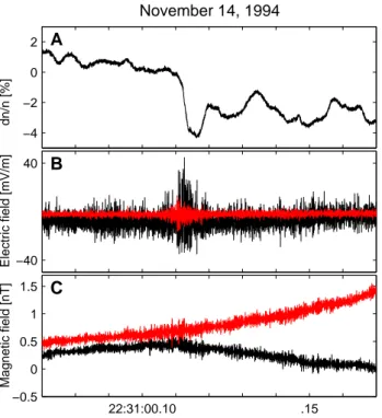
Fig. 1. Panel A shows the density variations observed along the satellite trajectory (perpendicular toB0).

The two recorded electric wave field components are shown in panel B. The black and red lines are the most perpendicular and the most parallel E-field component respectively. For both components we note a clear enhancement associated with the density gradient. In panel C corresponding magnetic wave fields are presented. Here the spin axis component (black line) has an angle of 77◦_to

B0and the spin plane component (red line)

has an angle of 43◦_to

B0. The increase in the magnetic wave activity is barely visible.

20

Fig. 1. Panel (A) shows the density variations observed along the satellite trajectory (perpendicular to B₀). The two recorded elec-tric wave field components are shown in panel (B). The black and red lines are the most perpendicular and the most parallel E-field components, respectively. For both components we note a clear enhancement associated with the density gradient. In panel (C) cor-responding magnetic wave fields are presented. Here the spin axis component (black line) has an angle of 77◦to B0and the spin plane

component (red line) has an angle of 43◦to B₀. The increase in the magnetic wave activity is barely visible.

similarities and differences between irregular density vari-ations and LHCs. As far as we are aware, this is the first satellite-based study detecting both magnetic and electric wave enhancements at small-scale density gradients.

The outline of this paper is as follows: first, we present two events where we find irregular density variations. They are examined in some detail in Sect. 3. A small statistical study based on 100 Freja orbits follows in Sect. 4. In Sect. 5 we investigate the wave activity surrounding both the irregular density variations and the LHCs.

2 Instrumentation and method

The Freja satellite was launched in October 1992 into an or-bit with apogee 1756 km, perigee 601 km and inclination 63◦, and provided almost three years of data (Lundin et al., 1994b; Lundin et al., 1998). This paper is based on data from the Freja wave instrument (F4) (Holback et al., 1994), which in-cluded six electrostatic probes mounted on wire booms in the spin plane, as well as a three-axis search coil magne-tometer. To achieve waveform resolution at high frequen-cies, a snapshot technique was used, where normally four

signals from these sensors were sampled at 4096 samples/s in brief intervals (typically 0.75 s every 4 s). At the same time, even shorter snapshots were sampled at 32 768 samples/s. In what was known as “burst mode”, up to five signals could be simultaneously sampled at 32 768 samples/s for some 15 s. These burst mode data, taken typically once or twice per day, form the basis of this study, as they allow for a detailed study of wave and plasma density variations.

The electrostatic probes could be used either in electric field mode, measuring voltage differences between probes fed with a constant bias frequency, or in Langmuir mode, sampling the current variations to a probe at constant bias voltage. For the plasma densities and density variation time scales we investigate here, the probe current variations are not significantly influenced by electric field fluctuations in a coupling capacity to the probe (Eriksson and Bostr¨om, 1998), and can be assumed to reflect variations in plasma density.

The ion data presented are obtained by the F3H hot plasma instrument (Eliasson et al., 1994) and the electron data are from the electron spectrometer (F7) (Boehm et al., 1994). The flux gate magnetometer F2 provides the background magnetic field (Zanetti et al., 1994).

3 Event studies

Density variations of a few percent are common at the Freja altitude. The cigar-shaped LHCs are well known. In this paper we focus on another type of density structure, which we will refer to as irregular density variations. In contrast to LHCs these density depletions are generally asymmetric and more or less one-sided. Furthermore, LHCs are associated with clear enhancements in the electric field only, while in most cases both the electric and the magnetic wave activity increase at the gradients of irregular density variations. 3.1 Event 1: 14 November 1994

Figure 1 presents time series data recorded by Freja on 14 November 1994. We show 0.2 s of data, including an ex-ample of the type of density variations we study. The event is observed at 1200-km altitude in the auroral region (MLT: 17.9 h, CGLAT: 67◦_{). In panel (A) the density variations}

along the satellite trajectory are displayed. For this case the spacecraft velocity is perpendicular to the background mag-netic field, B0. At 22:31:00.11 UT the density rapidly drops

about 4% but rises again about 0.01 s later. Hence, assuming a spatial structure and a satellite velocity of 7 km/s the width of this density depletion is approximately 70 m.

Panel (B) shows the two available electric field (E) com-ponents. The black line is the E-field component most per-pendicular to B0 while the red line depicts the component

most parallel to B0. The angles between B0and the

elec-tric field components are 23◦and 74◦, respectively. An en-hancement in the wave activity at the sharp gradient is clearly seen in both components. It can also be noted that the most

(mV/m) /Hz (nT) /Hz 0.05 0.1 0.15 0.2 0.25 2000 4000 6000 8000 10000 12000 14000 16000 time f (Hz) 1 1.5 2 2.5 3 3.5 4 4.5 5 PSD E−field vs time and frequency

−3 −2 −1 0 1 2 0.05 0.1 0.15 0.2 0.25 2000 4000 6000 8000 10000 12000 14000 16000 time f (Hz) −2 −1.5 −1 −0.5 0 0.5 1 Spectral density B−field vs time and frequency

0 10 20 30 40 50 60 70

PSD E−field vs. time and frequency Freja orbit 10172

f(kHz)

f(kHz)

t(s)

t(s) PSD B−field vs. time and frequency

log 10 ((mV/m) /Hz) 2 log 10 ((nT) 2/Hz) n dn_(%) dn n(%/km) 0.05 0.1 0.15 0.2 0.25 2000 4000 6000 8000 10000 12000 14000 16000 time f (Hz) 1 1.5 2 2.5 3 3.5 4 4.5 5 PSD E−field vs time and frequency

−4 −3 −2 −1 0 1 2 3 0.05 0.1 0.15 0.2 0.25 2000 4000 6000 8000 10000 12000 14000 16000 time f (Hz) −2 −1.5 −1 −0.5 0 0.5 1 Spectral density B−field vs time and frequency

0 10 20 30 40 50 60 Freja orbit 10172 f(kHz)

PSD B−field vs. time and frequency t(s)

t(s) PSD E−field vs. time and frequency

f(kHz) log 10 ((mV/m) 2/Hz) log 10 ((nT) 2/Hz) dn n(%/km) n dn_(%) 10 10 10 10 −8 −9 −7 −6 10 10 10 10 −6 −5 −4 −3 −2

A

B

November 14, 1994

Irregular density variation

Lower hybrid cavity

Fig. 2. The two large panels show seven seconds long electric and magnetic field spectrograms from November

14, 1994. At 22:31:00.5 UT the total density changes from 7900 cm−3 _{to 3100 cm}−3_{. The associated change}

in the lower hybrid cut-off frequency is marked with dashed lines in panel A. Before the density drop irregular density variations are found and after are LHCs detected. Enlarged are 0.3 seconds from two parts of the burst. The two top-left panels show an irregular density variation event and the two top-right panels show an LHC event.

21

Fig. 2. The two large panels show 7-s long electric and magnetic field spectrograms from 14 November 1994. At 22:31:00.5 UT the total density changes from 7900 cm−3to 3100 cm−3. The associated change in the lower hybrid cutoff frequency is marked with dashed lines in panel (A). Before the density drop irregular density variations are found and after are LHCs detected. Enlarged are 0.3 s from two parts of the burst. The two top-left panels show an irregular density variation event and the two top-right panels show an LHC event.

perpendicular component is larger throughout the time pe-riod shown.

In the bottom panel (C), the two recorded magnetic field (B) components are displayed and we can see a tendency toward an increase in the wave field at the gradient. The black line is the spin axis component, with an angle to B0

of 77◦, while the red line is a spin plane component with an angle of 43◦ to B0. There is no obvious difference in

amplitude between the two components.

Figure 2 shows a longer sequence from this burst. The two lower panels (A and B) display 7-s long electric and

magnetic field spectrograms. At 22:31:00.5 UT there is a sudden decrease in density. The consequent decrease of the lower hybrid cutoff frequency is evident in the electric field spectrogram (dashed lines in panel A). This feature turns out to separate two regions; irregular density variations are found before and LHCs are detected after the density decrease. The two types of density variations are exemplified in Fig. 2 by the enlarged sections. In the two top-left panels the density and the absolute value of the density gradient (black lines) are shown on top of the electric and magnetic field spectro-grams. Note that this is the same density variation as that

370 A. Reiniusson et al.: Wave field enhancements at density gradients

REINIUSSON ET AL.: WAVE FIELD ENHANCEMENTS AT DENSITY GRADIENTS 5

dn/n [%] A July 28, 1994 −2 0 2 | ∇ dn/n| [%/km] B 02:06:51.6 02:06:51.7 02:06:51.8 20 40 60 80 −5 −3 −1 f [Hz] log 10 [((mV)/m) 2/Hz] C 5000 10000 15000 −9 −7 −5 f [Hz] log 10 [(nT) 2/Hz] D 5000 10000 15000 P(E) [(mV/m) 2]x10−4 E 8960−11520 Hz 2.5 5.0 P(B) [(nT) 2] F 8960−11520 Hz x10−8 0 2 4 E/B [m/s] G 8960−11520 Hz x107 02:06:51.6 02:06:51.7 02:06:51.8 5 10 15 E/B [m/s] H 4480− 6400 Hz x108 02:06:51.6 02:06:51.7 02:06:51.8 0 4 8

Fig. 3. Panel A shows the density profile. Panel B displays the ab-solute value of the gradient of the density. We assume spatial struc-tures and the gradient is given in %/km. The electric and magnetic power spectral densities are plotted versus time and frequency in panels C and D. The electric and magnetic wave powers in the fre-quency range 8960–11520 Hz are given in panels E and F. Panels G and H presentE/B for the two frequency intervals 8960–11520 Hz

and 4480–6400 Hz.

10−1 100 101

July 28, 1994: Irregular density event E−field (E/E 0 ) 2 |∇ dn/n| [%/km] A 10−1 100 101 B−field (B/B 0 ) 2 |∇ dn/n| [%/km] B 0 10 20 30 40 50 60 70 10−1 100 101 E/B ((E/E 0 )/(B/B 0 )) 2 |∇ dn/n| [%/km] C

Fig. 4. Variations of the wave power for an irregular density varia-tion case. The analysis is based on 10 seconds of data from July 28, 1994, containing the three gradients presented in Fig. 3. Panel A and B show variations in the electric and magnetic wave power versus the gradient of the density, |∇dn/n|. The wave power is

normalized to the average wave power over the surrounding 0.5 s. Hence, a ratio larger than one means that there is an enhancement in the wave power. For steep gradients (|∇dn/n| & 30 %/km) we

see clear enhancements of both the electric and the magnetic wave power. Panel C presents the variation inE/B versus |∇dn/n|.

perimental studies (Eriksson et al., 1994) as well as with the theoretical model by Hall et al. (2004): even though the in-clusion of electromagnetic terms are crucial for understand-ing LHC wave properties below the lower hybrid frequency, fLH, the resulting wave fields are highly electrostatic in the sense ofE/B being very large.

3.2.2 Spatial structures

To check if the irregular density variations are spatial struc-tures we follow Holmgren and Kintner (1990) and cross cor-relate two density signals. Event 2 is suitable since we have two density signals that are recorded with a high sampling frequency during several seconds. Ifd is the probe distance along the satellite trajectory and λ is the observed wave-length, the phase difference between the two probes is ex-pressed as

h∆φi = 2πd

λ . (1)

We see from Eq. (1) that for stationary structures we get h∆φi ≈ 0 in the long wavelength limit. Moreover, for sta-Fig. 3. Panel (A) shows the density profile. Panel (B) displays the

absolute value of the gradient of the density. We assume spatial structures and the gradient is given in %/km. The electric and mag-netic power spectral densities are plotted versus time and frequency in panels (C) and (D). The electric and magnetic wave powers in the frequency range 8960–11 520 Hz are given in panels (E) and (F). Panels (G) and (H) present E/B for the two frequency intervals, 8960–11520 Hz and 4480–6400 Hz.

shown in Fig. 1, but here the time series of the density is smoothed. The two top-right panels show a LHC from a few seconds later.

Throughout the 7 s shown in panel (B), there is a clear emission at 10 kHz. These waves probably have a different wave mode than the background electrostatic waves. They are more electromagnetic and propagate presumably at a smaller angle to B0. Since this emission seems rather

un-affected by the local plasma properties, it may be suspected that the signal originates from a ground transmitter, such as the Omega stations transmitting at 10.2 kHz (Green et al., 2005; Kimura et al., 2001). However, a closer examina-tion reveals that the peak frequency varies between 9.5 and 11.5 kHz, and no amplitude variations corresponding to the ∼1-s pulses in the Omega signals can be discerned. We can-not rule out that this signal originally came from a ground transmitter, but, as will be discussed later in Sect. 6, most of the results presented in this paper would not be affected if this were the case.

3.2 Event 2: 28 July 1994

Event 1 is a unique example in our study including both ir-regular density variations and LHCs. Our next event con-tains only irregular density variations. We have already seen in Fig. 1 that magnetic field enhancements associated with these variations are difficult to spot in time series data. Usu-ally they are impossible to see, as the increase in amplitude is moderate and occurs in a limited frequency interval. How-ever, an increase in the magnetic wave activity may still be evident in time frequency spectrograms. Figure 3 provides an example of irregular density variations, where no enhance-ments in the B-field are seen in the time series data (not shown). We present 0.32 s of data recorded on 28 July 1994 (MLT: 18.8 h, CGLAT: 67◦). Panel (A) shows the density variations for this time period. The dashed lines mark three sharp gradients, where the density changes a few percent in 5–10 ms. In panel (B) the absolute value of the gradient of the density profile is plotted. We again assume that the vari-ations are spatial (cf. Sect. 3.2.2) and present the gradient in units of %/km. The three largest gradients have sizes of about 50 to 60%/km.

Panels (C) and (D) present the electric field and the mag-netic field spectrograms, respectively. We use only one E-field and one B-field component. The electric field is here almost perpendicular to B0 and the angle between B0

and the measured magnetic wave field component is 64◦_.

Wave emissions occur in the frequency range 5 kHz to at least 15 kHz. The sharp cutoff just below 5 kHz is interpreted as the lower hybrid cutoff. In the E-field spectrogram we see distinct enhancements in the spectral density at the marked gradients. The increases occur in a broad frequency band, ranging from just above the lower hybrid frequency cutoff to above 10 kHz. Enhancements in the B-field are also clearly visible (panel D). However, these enhancements are only vis-ible in the electromagnetic wave with frequencies around 10 kHz.

10−1 100 101

July 28, 1994: Irregular density event E−field (E/E 0 ) 2 |∇ dn/n| [%/km]

A

B

C

Fig. 4. Variations of the wave power for an irregular density variation case. The analysis is based on 10 seconds of data from July 28, 1994, containing the three gradients presented in Fig. ??. Panel A and B show variations in the electric and magnetic wave power versus the gradient of the density,|∇dn/n|. The wave power is normalized to the average wave power over the surrounding 0.5 s. Hence, a ratio larger than one means that there is an enhancement in the wave power. For steep gradients (|∇dn/n| & 30 %/km) we see clear enhancements of both the electric and the magnetic wave power. Panel C presents the variation inE/B versus |∇dn/n|.

23

Fig. 4. Variations of the wave power for an irregular density vari-ation case. The analysis is based on 10 s of data from 28 July 1994, containing the three gradients presented in Fig. 3. Panels (A) and (B) show variations in the electric and magnetic wave power versus the gradient of the density, |∇dn/n|. The wave power is normalized to the average wave power over the surrounding 0.5 s. Hence, a ratio larger than one means that there is an enhancement in the wave power. For steep gradients (|∇dn/n|&30%/km) we see clear enhancements of both the electric and the magnetic wave power. Panel (C) presents the variation in E/B versus |∇dn/n|.

To estimate the increase in wave power at these gradients we integrate the power spectral densities in the frequency range 8960–11 520 Hz. Our frequency resolution is 128 Hz and the interval is chosen to cover the 10-kHz-enhancement. The results are displayed in panels (E) and (F). We see that the power in the E-field is 10–20 times larger on the gradi-ents (panel E), although the increase in power close to the lower hybrid cutoff, particularly at the middle gradient, is not captured by the summation. The power in B is roughly doubled (panel F).

The two bottom panels show E/B for the two frequency intervals 8960–11 520 Hz and 4480–6400 Hz. The second interval is chosen to examine the wave activity around the lower hybrid frequency cutoff. In the higher frequency in-terval E/B is larger at the gradients. We conclude that the electrostatic wave is more enhanced here than the electro-magnetic wave. In the reference frequency interval, 4480– 6400 Hz, E/B is not correlated with the gradients.

10−1 100 101 September 3, 1993: LHC event E−field (E/E 0 ) 2 |∇ dn/n| [%/km] A 10−1 100 101 B−field (B/B 0 ) 2 |∇ dn/n| [%/km] B 0 20 40 60 80 100 120 140 10−1 100 101 E/B ((E/E 0 )/(B/B 0 )) 2 |∇ dn/n| [%/km] C

Fig. 5. Variations of the wave power for a LHC case. The analysis is based on 10 seconds of data observed on September 3, 1993. Analysis and panels are the same as in Fig. ??. All points with enhanced electric wave power and|∇dn/n| & 40 %/km are colored blue. From panel B we then see that there is no correlation between enhancements in the electric power and enhancements in the magnetic power.

24

Fig. 5. Variations of the wave power for an LHC case. The analysis is based on 10 s of data observed on 3 September 1993. Analysis and panels are the same as in Fig. 4. All points with enhanced elec-tric wave power and |∇dn/n|&40%/km are colored blue. From panel (B) we then see that there is no correlation between en-hancements in the electric power and enen-hancements in the magnetic power.

3.2.1 Irregular density variations versus LHCs

To prove that the enhancements of magnetic fields at density gradients in Figs. 1–3 are not isolated events, we systemat-ically analyze 10 s of data from this burst (28 July 1994). The entire time period is filled with irregular density varia-tions. Following the procedure leading to panel (E) in Fig. 3 we compute an electric wave power (∼E2) in the frequency range 8960–11 520 Hz. Then for each point in time the wave power is divided by a smoothed power (∼E2₀), obtained using a floating average over 500 points (∼0.5 s). In panel (A) of Fig. 4 (E/E0)2is plotted versus the magnitude of the density

gradient. We see that for weak gradients we have little sys-tematical variation of (E/E0)2, but for gradients&30%/km

the electric wave fields are enhanced. A horizontal dashed line is drawn at (E/E0)2=1 for reference. The result of the

corresponding analysis for the magnetic wave power is pre-sented in panel (B). We see that the magnetic wave power is also clearly enhanced for gradients_{&30%/km. The} enhance-ment in the magnetic wave power is, however, only about two times, while the electric wave power is often enhanced up to ten times. Hence, the ratio E/B, displayed in panel (C), also becomes larger for steep gradients.

372 A. Reiniusson et al.: Wave field enhancements at density gradients We conclude that there is an enhanced wave activity at the

gradients of irregular density variations. An increase in wave power is clear both for the electric and the magnetic wave fields. Simultaneously, the wave polarization changes, as we find a clear increase in E/B at the gradients. However, no changes can be detected in the polarization parameters E⊥/Ekor B⊥/Bk(not shown).

Figure 5 shows the corresponding analysis for an LHC case. The 10 s of data used are observed on 3 September 1993, beginning at 04:45:05.0 UT (see Eriksson et al., 1994 for time series and spectrograms of this event). At first it may be surprising that no clear increase in the E-field for large gradients is seen in panel (A). However, a closer in-spection reveals that there is a substantial number of cavities detected during the burst where no enhanced wave activity at all is observed. To investigate the wave-filled cavities fur-ther we concentrate on the cases where we see an increase in the electric wave power (blue dots in panel A), which is in approximately half of the cases. In Fig. 5 we see that the electric power for the LHC events can increase almost by a factor of ten. Panel (B) shows that there is no tendency of the magnetic wave power to increase when the density gra-dients steepen. Even if we consider only observations with a detected increase in electric power (blue dots), we see no ten-dency toward an enhancement in the magnetic power. This is in accordance with previous experimental studies (Eriks-son et al., 1994), as well as with the theoretical model by Hall et al. (2004): even though the inclusion of electromag-netic terms are crucial for understanding LHC wave prop-erties below the lower hybrid frequency, fLH, the resulting

wave fields are highly electrostatic in the sense of E/B being very large.

3.2.2 Spatial structures

To check if the irregular density variations are spatial struc-tures we follow Holmgren and Kintner (1990) and cross cor-relate two density signals. Event 2 is suitable since we have two density signals that are recorded with a high sampling frequency during several seconds. If d is the probe distance along the satellite trajectory and λ is the observed wave-length, the phase difference between the two probes is ex-pressed as

h1φi = 2π d

λ . (1)

We see from Eq. (1) that for stationary structures we obtain h1φi≈0 in the long wavelength limit. Moreover, for sta-tionary structures, all wavelength components should have equal phase (drift) velocities. If we have stationary struc-tures the frequencies we derive from our time series do not come from a true time variation but are inversely proportional to the wavelength of the static structures. Hence, we obtain f λ=vφ, where the phase velocity vφis constant and equal to

–vsat, where vsat is the satellite velocity relative to ground.

0 100 200 300 400 −200 −150 −100 −50 0 50 100 150 200 f [Hz] φ 1 − φ 2 [deg] July 28, 1994

Fig. 6. Phase difference versus frequency for two cross correlated density signals. The phase difference is small in the zero frequency limit. For low frequencies (long wavelengths) there is a good fit to a straight line, and the estimated phase velocity is just the satellite velocity with respect to Earth. The linear fit is made for data with a coherence above 0.5. Hence, we conclude that the density variations are spatial structures down to scale lengths of a few ion gyroradii (ρH+= 5–10 m, ρO+= 20–40 m). Data is taken from the same interval as the data shown in Fig. ??.

25

Fig. 6. Phase difference versus frequency for two cross correlated density signals. The phase difference is small in the zero frequency limit. For low frequencies (long wavelengths) there is a good fit to a straight line, and the estimated phase velocity is just the satel-lite velocity with respect to Earth. The linear fit is made for data with a coherence above 0.5. Hence, we conclude that the density variations are spatial structures down to scale lengths of a few ion gyroradii (ρ_H+=5–10 m, ρ_O+=20–40 m). Data is taken from the

same interval as the data shown in Fig. 3.

To check this assumption we use Eq. (1) to compute the drift velocity as

vφ=f λ =

2π d f

h1φi . (2)

Figure 6 presents the phase difference versus frequency. When computing the cross spectrum we used a record length of 1024 points and have averaged over 8 partly overlapping time records. The total time interval used is 0.1 s. For small frequencies (long wavelengths) the linear relationship be-tween the phase difference and the frequency is obvious and both criteria mentioned above are fulfilled.

The linear fit (red line) in Fig. 6 is made only for points with a coherence larger than 0.5 (see Holmgren and Kintner (1990) for details and arguments for doing so). The coher-ence can be interpreted as the correlation between the signals. From Fig. 6 we obtain a numerical value of f/h1φi. Us-ing the probe separation d=9 m, Eq. (2) gives |vφ|=7 km/s,

which equals the satellite speed relative to ground.

We notice that the correlation is good for frequencies up to 200 Hz. Since the relative speed between the satellite and the plasma is 7 km/s, this corresponds to structures larger than 35 m or an ion gyro radius (O+, 2 eV).

Thus, our analysis strongly indicates that the structures are truly spatial (down to a few ion gyroradii) and that the plasma drift velocity relative to ground is small, at least in the direc-tion parallel to the satellite velocity.

2.07.00 _{2.07.20 2.08.00} 19.2 68.7 18.8 18.9 19.1 68.4 67.7 67.0 + H e α energy (eV) energy (eV) 100 1000 100 10000 1000 10 log(cts/s) 3.0 4.2 3.6 CGLAT MLT UT − 2.07.40 1.8 2.8 2.3 July 28, 1994

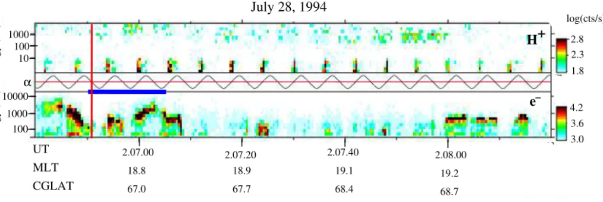
Fig. 7. Particle observations from July 28, 1994. The time interval corresponding to the wave data presented

in Fig. ?? is indicated with a thick red line. The top panel shows count rates of H+ versus time, while the corresponding pitch angles are displayed in the middle panel. Since the data are recorded in the northern hemisphere a pitch angle of 0◦_{(i.e., parallel to the ambient magnetic field) corresponds to downgoing particles.}

The bottom panel displays count rates of downgoing electrons. Irregular density variations with enhancements in the wave E- and B-fields are found at the edge of an inverted-V structure.

26

Fig. 7. Particle observations from 28 July 1994. The time interval corresponding to the wave data presented in Fig. 3 is indicated with a thick red line. The top panel shows count rates of H+versus time, while the corresponding pitch angles are displayed in the middle panel. Since the data are recorded in the Northern Hemisphere a pitch angle of 0◦(i.e. parallel to the ambient magnetic field) corresponds to downgoing particles. The bottom panel displays count rates of downgoing electrons. Irregular density variations with enhancements in the wave E- and

B-fields are found at the edge of an inverted-V structure.

3.2.3 Particle observations

Using information from the Freja particle detectors we can characterize the plasma environment in which irregular den-sity variations are found. Figure 7 shows 100 s of proton and electron overview data. Proton count rates, from the TICS ion spectrometer of the F3H instrument, obtained by adding data from two neighboring mass spectrometer angular sec-tors directed nearly perpendicularly to the satellite spin axis, are shown in the top panel. As the spacecraft rotates the detector points in different directions relative to the back-ground magnetic field. The pitch angles of the detected pro-tons are shown in the middle panel. As the observations are made in the Northern Hemisphere, a pitch angle of 0◦ cor-responds to downgoing protons. The bottom panel presents the downgoing electrons observed by the TESP (F7) detec-tor. Both at the beginning and at the end of the interval, the so-called inverted-V electrons are present. The energy of these downward accelerated electrons is about 1 keV. Our data indicate that inverted-V structures are more or less anti-correlated with a weak signature of downgoing protons with keV energies, suggesting that the spacecraft might be enter-ing a return current region. The low energy ions observed once every satellite spin (every 6 s) are heavier ions, mainly O+, recorded due to the satellite ram effect. This is a reoc-curring feature in all F3H/TICS data.

The vertical red line in Fig. 7 shows the time of the burst mode wave data previously presented in Fig. 3. The en-tire burst is 15 s long (02:06:45–02:07:00 UT, marked with a horizontal blue line) and spatial irregular density variations are recorded throughout this time interval. We conclude that density variations with enhanced E- and B-fields at the gra-dients in this case are observed at the edge of an inverted-V electron structure, close to a presumed return current region.

4 Statistics

To examine how often irregular density variations and LHCs occur we made a statistical study. As waves above 2 kHz are covered for substantial time intervals only when the F4 in-strument is in its burst mode, our data set is limited to all F4 bursts. The total number of available bursts in proper burst modes, with one density measurement, two E- and two B-components, is 100, each 10–15 s long. The reason for choosing this burst mode is that we need as many field components as possible to study the polarization of the back-ground waves.

To sort out the data of interest we first eliminate all bursts without density variations of at least 1% over a few ion gyroradii. We also eliminate events with an electric wave amplitude, above the lower hybrid frequency, of less than 1 mV/m. After these eliminations only 13 of the 100 bursts remain. To classify a burst as an LHC event we demand repeated Gaussian-shaped density depletions with widths of 50–100 m. We find that six of our 13 bursts fulfill these cri-teria. In studies by, for example, Høymork et al. (2000), Dovner et al. (1994), Eriksson et al. (1994), Tjulin et al. (2003), Schuck et al. (2003) and Knudsen et al. (1998) the same criteria have been used to classify LHCs. Six of the remaining seven bursts have density variations that are irreg-ular and do not fulfill the criterias for LHC events. We call these events irregular density variation events. These type of structures are also investigated by, for example, Temerin (1978), Delory et al. (1997), Fejer and Kelley (1980), Saga-lyn et al. (1974) and Holmgren and Kintner (1990). Finally, the last burst, Event 1, includes both LHCs and irregular density variations (see Fig. 2). In this statistical study we also include Event 2, which is recorded in a different burst mode giving two density measurements, two E- and one B-components. We needed an event with two density measure-ments to verify that the structures are spatial (see Sect. 3.2.2). In Table 1 we show some properties of our 14 (13+ Event 2) events. In the first five columns we present the type

374 A. Reiniusson et al.: Wave field enhancements at density gradients

Table 1. Properties of detected irregular density variation events and LHC events. The densities are determined from the plasma frequency in all cases except one. In event 94.06.05 the density is determined from the fLH, where we assumed 95% O+and 5% H+. In the seventh

column the energetic electrons are characterized. The events where the B-field is enhanced on the gradients of the density variations can be seen in the last column. Event 2 from 28 July 1994, is measured in a different burst mode than the rest, with two density signals, two E- and one B-component.

TYPE DATE start time MLT CGLAT DENSITY Electrons Enhancement in B

[yy.mm.dd] [UT] [hours] [◦] [#/cm3]

Irregular density variation 93.09.30 22:55:51.1 17.7 66 4000 Inverted-V Yes

events 94.03.31 03:47:13.2 23.5 67 2500 Inverted-V Yes

94.04.16 01:09:12.7 21.1 72 2500 Inverted-V Yes

94.04.21 22:43:24.7 18.7 67 3100 Inverted-V Yes

94.07.28 02:06:50.5 18.8 67 2500 Inverted-V Yes

94.11.25 20:12:06.7 21.1 59 7900 Radiation belt No

95.02.07 05:18:12.1 1.6 73 6000 Inverted-V No

Irregular density variation 94.11.14 22:30:57.8 17.9 67 7900/3100 Inverted-V Yes/No

event/LHC event

LHC events 93.09.03 04:45:05.9 5.9 60 1700 Radiation belt No

94.04.06 03:11:29.9 21.0 64 800 Inverted-V No

94.04.10 03:27:20.6 19.9 64 800 Inverted-V No

94.05.15 16:46:31.3 11.4 57 800 Radiation belt No

94.06.05 12:24:01.0 13.0 61 3300 Radiation belt No

95.03.02 23:26:59.0 21.0 70 1300 Inverted-V No

of density variation, the date of the recorded data, the start time in UT for the bursts, MLT and CGLAT, respectively. The events with enhanced magnetic wave fields at density gradients are listed in the last column. We see that this occurs only for the irregular density variation events. None of our LHC events has enhanced magnetic wave activity at the den-sity gradients, which is expected, since several other studies (see, e.g. Høymork et al., 2000; Dovner et al., 1994; Eriks-son et al., 1994) have arrived at the same result. Note that Event 1 (94.11.14) is marked with Yes/No. In the first few seconds of that event we find only irregular density varia-tions with magnetic field enhancements on its gradients. In the latter part there are LHCs, and no density gradient B-field enhancements are recorded (see Fig. 2).

In column six we display the electron density, which is estimated from the electron plasma frequency. We find that the density is generally higher for irregular density variation events than for LHC events. In Event 1 the densities are dif-ferent in regions with irregular density variations and LHCs. This is also reflected in the changing fLHcutoff in panel (A)

in Fig. 2.

From the seventh column of Table 1 we see that all irreg-ular density variation events with enhanced magnetic field are related to accelerated auroral electrons. They are gen-erally at the edge of a so-called inverted-V structure, where the electron energies are moderate, rarely above a few keV. Such downgoing electrons are also found during all our LHC

events on the nightside, while the LHC events on the dayside at lower latitudes are found in the radiation belt, which is characterized by energetic electrons in the MeV range. Even though we do not have an instrument designed for measur-ing these electrons we can still easily identify them. They can penetrate the ion instrument and cause an artificial signal evenly spread over all ion energy levels. This is a characteris-tic signature in the data and easy to identify. For most events we have used the TESP electron data to identify inverted-V electrons (see, e.g. the electron panel in Fig. 7). For a few of the latter events, when TESP was no longer functional, we used data from the MATE electron instrument. MATE have no energy resolution, but we can still, from the time series of the total electron count rate, integrated over the electron ener-gies 0.1–120 keV, make a reliable identification of inverted-V events.

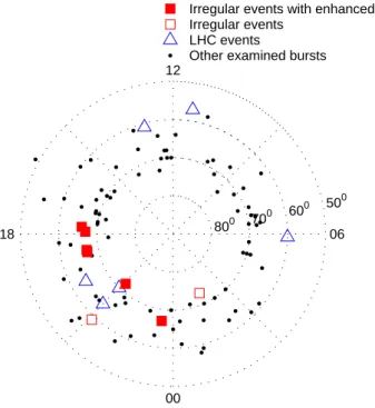
To visualize the results from Table 1 we construct Fig. 8, which shows the Northern Hemisphere above 50◦ CGLAT, where all the investigated bursts are marked. Irregular den-sity variation events are marked by squares and LHC events by triangles. Filled symbols indicate events with enhanced magnetic wave activity. Event 1, which includes both ir-regular density variations and LHCs, is marked by a filled square. Freja bursts, not classified as one of the types above, are marked by dots.

We see from Fig. 8 that irregular density variation events and LHC events are approximately equally common in our

18 00 06 12 800 70 0 600 50 0

Irregular events with enhanced B Irregular events

LHC events

Other examined bursts

Fig. 8. View over the northern hemisphere. The time is given in MLT and the circles indicate the latitude. Due to the 63◦ _{inclination of the Freja orbit we do not measure above 75}◦_{. Irregular density variation events are}

marked by squares. The filled squares indicate where events with enhanced magnetic wave activity has been found. Triangles denote LHC events, while dots mean that no density variations are detected. Event 1, that includes both irregular density variations and LHCs, is marked by a filled square.

27

Fig. 8. View over the Northern Hemisphere. The time is given in MLT and the circles indicate the latitude. Due to the 63◦ incli-nation of the Freja orbit we do not measure above 75◦. Irregular density variation events are marked by squares. The filled squares indicate where events with enhanced magnetic wave activity have been found. Triangles denote LHC events, while dots mean that no density variations are detected. Event 1, which includes both irregular density variations and LHCs, is marked by a filled square.

study. The irregular density variation events are located in the pre-midnight sector in the high-latitude auroral region. We find LHC events in the same region but also on the day-side at lower latitudes. This is in agreement with the statisti-cal study of the locations of LHC events at the Freja altitude by Dovner et al. (1997), which was not limited to the F4 bursts and hence based on a much larger data set.

5 Wave model

Complete knowledge of the properties of the background waves is important to understand the coupling processes be-tween the gradients/cavities and the waves. Such information is also essential for investigating if interactions between the plasma and the waves are responsible for creating the differ-ent kinds of density structures.

We return to Event 1, in order to investigate the nature of the waves in the two different regions there. We model the plasma and use the dispersion solver WHAMP (R¨onnmark, 1982). As we aim to describe the waves outside the cavities or gradients, the theory of linear waves in a homogeneous plasma should be applicable. The models used are summa-rized in Table 2. We assume a quasi-neutral oxygen dom-inated plasma (O+ 95%, H+ 5%), where all ions are non-drifting and cold (2 eV). The electrons are modeled using two

Table 2. The plasma models used in the high (NH) and low density

(N_L) cases. Four plasma components are used. The background plasma is regarded as cold (2 eV) and oxygen dominated (O+95%, H+5%). In addition, we assume 5% downgoing 1 keV inverted-V electrons, whose drift velocity equals the thermal velocity. In Table 2 the drift velocity is normalized to the thermal velocity. The total density is 7900 cm−3in the high density case and 3100 cm−3 in the low density case. For both cases f_H+=514 Hz.

SPECIES NH NL Tk T⊥ DRIFT [cm−3] [cm−3] [eV] [eV] [–] H+ 400 155 2 2 0 O+ 7500 2945 2 2 0 e− 7500 2945 2 2 0 e− 400 155 1000 1000 1 10−4 10−3 10−2 10−1 100 k_⊥ρ H+ −k || ρ H +

A

B

Fig. 9. Constant frequency curves in wave vector space. The parallel and perpendicular wave vectors are normalized to the gyro radius of the 2 eV protons in the models, that is ρ_H+= 7m. Panel A is the results from

modelling the high density case, where irregular density events are present. Panel B is the dispersion curves for the low density case. The overall structure is very similar. We can note a small shift of a curve at a given frequency towards larger k for a higher density.

28

Fig. 9. Constant frequency curves in wave vector space. The paral-lel and perpendicular wave vectors are normalized to the gyroradius of the 2-eV protons in the models, that is ρ_H+=7 m. Panel (A)

shows the results from modelling the high density case, where ir-regular density events are present. Panel (B) shows the dispersion curves for the low density case. The overall structure is very similar. We can note a small shift in a curve at a given frequency towards larger k for a higher density.

components, a cold ionospheric component and hot inverted-V electrons drifting parallel to B0. The drifting electrons

constitute 5% of the total electron density and their drift ve-locity is equal to their thermal veve-locity. The total density in

376 A. Reiniusson et al.: Wave field enhancements at density gradients 10−3 10−2 10−1 100 k_⊥ρ H+ −k || ρ H + A High density 70° 63° 74° 15000 Hz 10000 Hz 5000 Hz 10−3 10−2 10−1 100 k_⊥ρ H+ −k || ρ H + B Low density 31° 33° 79° 15000 Hz 10000 Hz 3500 Hz 10−4 10−2 100 10−20 10−15 10−10 k_⊥ρ H+ WDF [arbitrary units] C High density 15000 Hz 10000 Hz 5000 Hz 10−4 10−2 100 10−20 10−15 10−10 k_⊥ρ H+ WDF [arbitrary units] D Low density 15000 Hz 10000 Hz 3500 Hz

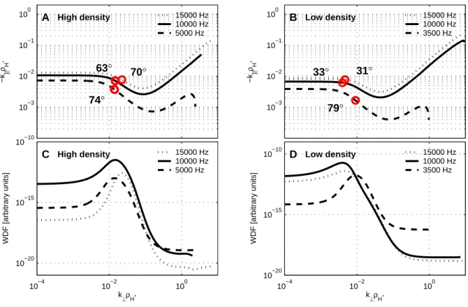
Fig. 10. The peaks in the reconstructed WDF are presented on top of constant frequency curves in wave vector

space in panels A and B. In panels C and D the WDF is plotted versus normalized k⊥. As before ρH+ = 7m.

29

Fig. 10. The peaks in the reconstructed WDF are presented on top of constant frequency curves in the wave vector space in panels (A) and (B). In panels (C) and (D) the WDF is plotted versus normalized k⊥. As before ρH+=7 m.

the two cases is 3100 cm−3and 7900 cm−3, respectively. The background magnetic field is approximately 33 800 nT, giv-ing an electron gyrofrequency of 945 kHz. The lower hybrid frequency in the modeled plasma is 3800 Hz and 6100 Hz for the two cases, in agreement with Fig. 2. In the frequency range of interest – above the lower hybrid frequency and below both the electron gyrofrequency and the plasma fre-quency – the only continuous wave mode with a significant magnetic component is the whistler mode. Thus, only this mode is considered in the following analysis.

The mode structure is presented in Fig. 9. At a given fre-quency an existing wave mode appears as a curve in wave vector (k) space. Figure 9 presents three such constant fre-quency curves in k-space for each case. The parallel and perpendicular wave vectors are normalized to the inverse of the gyroradius of the 2 eV protons in the models, that is ρH+=7 m. We observe that the overall structure is very sim-ilar. Comparing a curve at a given frequency, say 10 kHz, in the two different plasmas we note a slight shift in k-space.

Polarization parameters, such as E/B, E⊥/Ek and

B⊥/Bk, vary along the constant frequency curves. Hence,

by comparing the observations with the theoretical model we can determine where along the curves most of the wave en-ergy is localized. To do this in a systematic way we use Wave Distribution Function (WDF) analysis (Storey and Lefeuvre, 1974; Oscarsson and R¨onnmark, 1989). The idea is to use all the available polarization information (e.g. the amplitude

and phase relations between the measured field components) to determine the wave energy distribution in wave vector space. Details of the algorithm used can be found in Oscars-son (1994). Stenberg et al. (2002) provide an application of the method. WDF analysis is especially useful in this case, where we only have two electric and two magnetic field com-ponents and where conceptually simpler plane wave methods cannot easily be applied.

The results from the WDF analysis are presented in Fig. 10. The constant frequency curves in panels (A) and (B) are the same as in Fig. 9. The red circles on top of these curves denote the peaks in the reconstructed wave energy distributions. For clarity the angle between the wave vec-tor and the background magnetic field is presented next to each peak. We see that the wave energy is most probably located at similar wave vectors in the low and high density cases. In the low density case, waves at higher frequen-cies (10 and 15 kHz) propagate more parallel to the ambient field than waves closer to the lower hybrid cutoff frequency (3.5 kHz). This confirms the assumption made in Sect. 3.1 that we observe a mix of a more parallel propagating elec-tromagnetic wave at frequencies around 10 kHz and oblique electrostatic emissions. However, in the high density case the WDF technique does not distinguish between the two wave modes. Waves at all frequencies seem to propagate at a large angle to B0.

Panels (C) and (D) show the reconstructed WDF versus normalized k⊥. It is worth noting that the peaks are very

pro-nounced, which indicates that the polarization information in the data is sufficient to pinpoint the wave energy in k-space. From the WDF reconstructions we estimate the perpendicu-lar wavelengths for the high density case to roughly 1500– 4000 km, which is much larger than the small-scale density variations we study. The wavelength is somewhat longer for the low density (LHC) case. From this analysis we find that the waves truly are very similar in the two regions. None of the polarization parameters change much, and the waves are located at similar wave vectors. The perpendicular wave-lengths are much longer than the size of the density struc-tures. For both cases examined the waves are found to be electromagnetic whistler mode waves rather than more elec-trostatic waves located on the resonance cone. Hence, at least in this event, the LHCs are not fed with electrostatic waves, as is often assumed (Schuck et al., 2003).

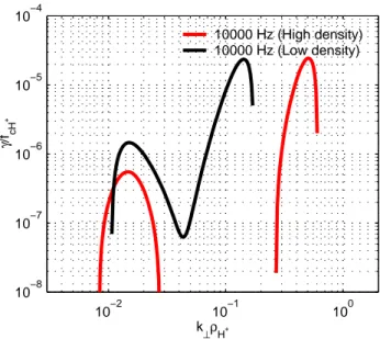
Finally, we should note that both plasma models used (cf. Table 2) contain a source of free energy, namely the field-aligned electrons. These electrons are responsible for weak instabilities both at the wave vectors, where we believe the wave energy is located, and at larger perpendicular wave vec-tors. The location of the instabilities in wave vector space at 10 kHz is shown in Fig. 11. The instabilities at larger k⊥

correspond to wavelengths of 70–300 m, which are compa-rable to the sizes of the density structures. Therefore, since all irregular density variations analyzed in the present study are accompanied by inverted-V electrons, we cannot exclude a possible connection between the instability and the forma-tion of these density structures. On the other hand, this ar-gument is not valid for LHCs which also exist in the absence of inverted-V electrons. Therefore, the significance of the instability is unclear.

We conclude that the background waves are similar irre-spective of the type of density variations observed. These waves have wavelengths much longer than the typical density structures. It has been suggested that such long wavelength waves can interact with existing small-scale density varia-tions to excite short wavelength electrostatic waves (Bell and Ngo, 1990). Another possibility is that the instability shown in Fig. 11 constitutes the seed for the initiation of the density structures themselves.

6 Discussion

In this paper we have studied electric and magnetic waves lo-calized on small-scale density gradients. A number of previ-ous studies of this phenomenon have focused on waves asso-ciated with LHCs. We have instead focused on waves found together with irregular density structures. On the gradients of such structures we find enhancements in both the electric and the magnetic wave activity. This is in contrast to most inves-tigations of LHCs, where only the electric power increases in the cavities. A rocket observation reported by D. Knudsen (private communication) is, as far as we know, the only case

10−2 10−1 100 10−8 10−7 10−6 10−5 10−4 k_⊥ρ_H+ γ /f cH + 10000 Hz (High density) 10000 Hz (Low density)

Fig. 11. The temporal growth rate versus k⊥ρ+H(ρH+= 7m). In both the high (red lines) and low density

(black line) cases there are two peaks in growth rate, one at the perpendicular wave vector where we believe most of the wave energy to be located and one at larger k⊥.

30

Fig. 11. The temporal growth rate versus k⊥ρ_H+ (ρ_H+=7 m). In

both the high (red lines) and low density (black line) cases there are two peaks in the growth rate, one at the perpendicular wave vector, where we believe most of the wave energy to be located, and one at larger k⊥.

where there are also enhancements in the magnetic wave ac-tivity associated with LHCs.

We have found that the densities are considerably higher for irregular density variation events than for LHC events. Also, the shape of the density variations differs between the two event types. These two features might explain the dif-ference in nature between the enhanced waves on the density gradients.

Furthermore, we see from Figs. 4 and 5 that the electric field almost always is enhanced on the large gradients of the irregular density variations, but only on about half of the large LHC gradients. However, we have examined only a few events and the confirmation of the observations will be included in a future study.

The presence of inverted-V electrons near the irregular density variations suggests that whistler waves are at least marginally unstable near 10 kHz. Hence, the narrow band emission shown in panel (b) in Fig. 2 may be caused by a space plasma instability, but since man-made signals are ubiquitous in the magnetosphere we cannot rule out that it originated from a ground transmitter. However, the origin of the waves should not affect how they interact with the irreg-ular density variations. In particirreg-ular, the enhancement of the wave magnetic field on the gradients of the irregular density variations are not explained by assuming that the waves come from a ground-based radio transmitter.

In laboratory experiments, waves localized in density de-pletions have ∇×E6=0. Thus, they are electromagnetic (see, for example, Rosenberg and Gekelman, 2001). There are discussions about whether the conditions in the laboratories are similar to those for LHCs in space (Schuck et al., 2004;

378 A. Reiniusson et al.: Wave field enhancements at density gradients Gekelman, 2004). The shape of the depletions are

some-what different. This might explain the different nature of LHCs and waves measured in laboratories. The conditions in laboratories are in certain respects more similar to irregu-lar density variation events. We do not claim that the waves in laboratories are of the same type as the waves we measure but do not exclude that they are related.

7 Conclusions

In this paper we focus on small-scale irregular density varia-tions observed by the Freja satellite at 1000–1700 km in the auroral zone. The main conclusions are summarized below:

- Irregular density variations in an environment of whistler mode/lower hybrid waves are quite common at the Freja altitude. The variations we observe are spatial structures with a very low drift velocity. If the gradi-ents of the density structures are steep enough, both the electric and magnetic wave fields are usually enhanced. - In a small statistical study we find that irregular density variations and LHCs occur equally as often. Generally, the observed densities are higher when we record irreg-ular density variations than when LHCs are detected. - Gradients with enhanced electric and magnetic wave

fields are found in the pre-midnight sector (MLT 18:00– 00:00). Generally, they are found at the edges of inverted-V electron structures, and sometimes very close to return current regions, indicated by downgoing keV protons.

- The background waves are electromagnetic (E/B≈5·107m/s at 10 kHz) whistler mode waves. The wavelengths are of the order of 1.5–4.0 km, which is much larger than the typical size of the density structures. At the gradients we observe a significant in-crease in E/B, indicating that the localized waves have much shorter wavelengths. Similar electromagnetic background waves are also observed in the LHC case investigated.

Acknowledgements. The authors thanks J. O. Hall and H. P´ecseli

for useful discussions. We also acknowledge Freja PIs for providing data. A. Reiniusson is supported by the Swedish National Graduate School of Space Technology.

Topical Editor I. A. Daglis thanks two referees for their help in evaluating this paper.

References

Andr´e, M. (Ed.): The Freja scientific satellite, IRF Scientific Report 214, Swedish Institute of Space Physics, Kiruna, 1993.

Bamber, J. F., Maggs, J. E., and Gekelman, W.: Whistler wave in-teraction with a density striation: A laboratory investigation of an auroral process, J. Geophys. Res., 100, 23 795–23 810, 1995.

Bell, T. F. and Ngo, H. D.: Electrostatic lower hybrid waves ex-icited by electromagnetic whistler mode waves scattering from planar magnetic-field-aligned plasma density irregularities., J. Geophys. Res., 95, 149–172, 1990.

Boehm, M., Paschmann, G., Clemmons, J., et al.: The TESP elec-tron spectrometer and correlator (F7) on Freja, Space Sci. Rev., 70, 509–540, 1994.

Delory, G. T., Ergun, R. E., Klementis, E. M., et al.: Measurements of short wavelength VLF bursts in the auroral ionosphere: A case for electromagnetic mode conversion?, Geophys. Res. Lett., 24, 1131–1134, 1997.

Dovner, P. O., Eriksson, A. I., Bostr¨om, R., et al.: Geophys. Res. Lett., 21, 1827–1830, 1994.

Dovner, P. O., Eriksson, A. I., Bostr¨om, R., et al.: Geophys. Res. Lett. 24, 619–622, 1997.

Eliasson, L., Norberg, O., Lundin, R., et al.: The Freja hot plasma experiment: Instrument and first results, Space Sci. Rev., 70, 563–576, 1994.

Eriksson, A. I., Holback B., Dovner, P. O., et al.: Geophys. Res. Lett., 21, 1843–1846, 1994.

Eriksson, A. and Bostr¨om, R.: Wave measurements using electro-static probes: accuracy evaluation by means of a multiprobe tech-nique, Measurement techniques in space plasmas: Fields (AGU geophysical monograph 103), American Geophysical Union, 147–153, 1998.

Gekelman, W.: Comment on ”Properties of lower hybrid soli-tary structures: A comparison between space observations, a laboratory experiment and the cold homogeneous plasma dis-persion relation” by Schuck et al., J. Geophys. Res., 109, doi:10.1029/2002JA009778, 2004.

Green, James L., Boardsen S., Garcia L., et al.: On the origin of whistler mode radiation in the plasmasphere, J. Geophys. Res., 110, doi:10.1029/2004JA010495, 2005.

Fejer, B. G. and Kelley, M. C.: Ionospheric irregularities, Rev. Geo-phys., 18, 401–454, 1980.

Hall, J. O., Eriksson, A. I., and Leyser, T. B.: Excitation of localized rotating waves in plasma density cavities by scattering of fast magnetosonic waves, Phys. Rev. Lett. 92, Art. No. 255002, 2004. Holmgren, G. and Kintner, P. M.: Experimental Evidence of Widespread Regions of Small-Scale Plasma Irregularities in the Magnetosphere, J. Geophys. Res., 95, 6015–6023, 1990. Holback, B., Jansson, S.-E., ˚Ahl´en, L., et al.: The Freja wave and

plasma density experiment, Space Sci. Rev., 70, 577–592, 1994. Høymork, S. H., P´ecseli, H. L., Lybekk, B., et al.: Cavitation of Lower-Hybrid Waves in the Earth’s ionosphere; a model analy-sis, J. Geophys. Res., 105, 18 519–18 535, 2000.

Kimura, I., Kasahara, Y., and Oya, H.: Determination of global plasmaspheric electron density profile by tomographic approach using omega signals and ray tracing, J. Atmos. S.-P., 63, 1157– 1170, 2001.

Knudsen, D. J., Dovner, P. O., Eriksson, A. I., et al.: Effect of lower hybrid cavities on core plasma observed by Freja, J. Geophys. Res., 103, 4241–4249, 1998.

Lundin, R., Haerendel, G., and Grahn, S.: The Freja Project, Geo-phys. Res. Lett., 21, 1823–1826, 1994a.

Lundin, R., Haerendel, G., and Grahn, S.: The Freja science mis-sion, Space Sci. rev., 70, 405–419, 1994b.

Lundin, R., Haerendel, G., and Grahn, S.: Introduction to special section: The Freja mission, J. Geophys. Res., 103, 4119–4123, 1998.

Oscarsson, T.: Dual Principles in Maximum Entropy Reconstruc-tion of the Wave DistribuReconstruc-tion FuncReconstruc-tion, J. Comput. Phys., 110,

221–233, 1994.

Oscarsson, T. and R¨onnmark, K.: Reconstruction of wave distri-bution functions in warm plasmas, J. Geophys. Res., 94, 2417– 2427, 1989.

Rosenberg, S. and Gekelman, W.: A three-dimensional experimen-tal study of lower hybrid wave interactions with field-aligned density depletions, J. Geophys. Res., 106, 28 867–28 884, 2001. R¨onnmark, K.: WHAMP – Waves in Homogeneous Anisotropic

Multicomponent Plasmas, KGI Report 179, Kiruna Geophysical Institute, 1982.

Sagalyn, R. C., Smitty, M., and Ahmed, M.: High-latitude irregu-larities in the topside ionosphere based on Isis 1 thermal probe data, J. Geophys. Res., 79, 4252–4261, 1974.

Schuck, P. W., Bonnell, J. W., and Kintner, P. M.: A Review of Lower Hybrid Solitary Structures, IEEE Trans. Plasma Sci., 31, 1125–1177, 2003.

Schuck, P. W., Bonnell, J. W., and Pinc¸on, J.-L.: Properties of lower hybrid solitary structures: A comparison between space observations, a laboratory experiment and the cold ho-mogeneous plasma dispersion relation, J. Geophys. Res., 109, doi:10.1029/2002JA009673, 2004.

Sonwalkar, V. S., and Harikumar, J.: An explanation of ground ob-servations of auroral hiss: Role of density depletions and meter-scale irregularities, J. Geophys. Res., 105, 18 867–18 883, 2000. Stenberg, G., Oscarsson, T., Andr´e, M., et al.: Investigat-ing wave data from the FAST satellite by reconstructInvestigat-ing the wave distribution function, J. Geophys. Res., 107, doi: 10.1029/2001/2001JA900154, 2002.

Storey, L. R. O., and Lefeuvre, F.: Theory for the interpretation of measurements of the six components of a random electromag-netic wave field in space, Space Res., 14, 381–386, 1974. Temerin, M.: The polarization, frequency and wavelengths of

high-latitude turbulence, J. Geophys. Res., 83, 2609–2616, 1978. Tjulin, A., Eriksson, A. I., and Andr´e, M.: Lower hybrid

cav-ities in the inner magnetosphere, Geophys. Res, Lett., 30, doi:10.1029/2003GL016915, 2003.

Zanetti, L. and the Freja Magnetic Field Experiment Team: Mag-netic field experiment on the Freja satellite, Space Sci. Rev., 70, 465–482, 1994.