HAL Id: hal-00317729
https://hal.archives-ouvertes.fr/hal-00317729
Submitted on 29 Nov 2004
HAL is a multi-disciplinary open access
archive for the deposit and dissemination of
sci-entific research documents, whether they are
pub-lished or not. The documents may come from
teaching and research institutions in France or
abroad, or from public or private research centers.
L’archive ouverte pluridisciplinaire HAL, est
destinée au dépôt et à la diffusion de documents
scientifiques de niveau recherche, publiés ou non,
émanant des établissements d’enseignement et de
recherche français ou étrangers, des laboratoires
publics ou privés.
scheme and velocity comparisons
D. A. Holdsworth, I. M. Reid
To cite this version:
D. A. Holdsworth, I. M. Reid. The Buckland Park MF radar: routine observation scheme and velocity
comparisons. Annales Geophysicae, European Geosciences Union, 2004, 22 (11), pp.3815-3828.
�hal-00317729�
SRef-ID: 1432-0576/ag/2004-22-3815 © European Geosciences Union 2004
Annales
Geophysicae
The Buckland Park MF radar: routine observation scheme and
velocity comparisons
D. A. Holdsworth1,2and I. M. Reid2
1Atmospheric Radar Systems, 1/26 Stirling St, Thebarton, South Australia, Australia
2Department of Physics and Mathematical Physics, The University of Adelaide, South Australia, Australia
Received: 1 October 2003 – Revised: 18 December 2003 – Accepted: 9 January 2004 – Published: 29 November 2004 Part of Special Issue “10th International Workshop on Technical and Scientific Aspects of MST Radar (MST10)”
Abstract. This paper describes the routine observations scheme implemented for the Buckland Park medium fre-quency (BPMF) radar. These observations are rare among current MF/HF radar observations in that they are made us-ing a relatively narrow transmit polar diagram. The flexibility of the radar allows a number of analyses to be performed si-multaneously. The analyses described include the full corre-lation analysis (FCA), spatial correcorre-lation analysis (SCA), hy-brid Doppler interferometry (HDI) and imaging Doppler in-terferometry (IDI) for observations of mesospheric dynamics and the temporal and spatial characteristics of their scatter-ers, the differential absorption experiment (DAE) for the es-timation of electron densities and collision frequencies, and meteor analysis for estimation of meteor height, time and an-gle of arrival (AOA) distributions. Intercomparisons between wind velocities estimated using the FCA with SCA, HDI and IDI techniques are presented. The FCA velocities exhibit the well-known “triangle size effect” (TSE), whereby the wind velocity is underestimated at smaller antenna spacings. Al-though the SCA, IDI and HDI techniques were not applied concurrently, comparisons using FCA as a reference suggest these techniques produce velocities in good agreement.
Key words. Ionosphere (instruments and techniques) –
Me-teorology and atmospheric dynamics (instruments and tech-niques) – Radio science ( instruments and techtech-niques)
1 Introduction
Medium (MF) and high frequency (HF) radars are capable of providing continuous height coverage between 60 and 100 km during the day and 80 and 100 km at night (e.g. Hocking, 1997b). Although MF/HF radars have limited range resolution due to the relatively long wavelengths used (e.g. λ=150 m at 2 MHz), they are ideal for routine obser-vations, allowing continuous measurements of winds for
es-Correspondence to: D. A. Holdsworth
timation of waves, tides and turbulence. The majority of MF/HF radars used for routine observations are “spaced an-tenna” (SA) systems, consisting of a small transmitting array and a number of spaced antennas for reception (e.g. Vincent and Lesicar, 1991).
Until recently, routine spaced antenna observations made using the Buckland Park MF (BPMF) radar were carried out in a similar manner. The original radar used a small trans-mitting array and a large 1-km diameter array for reception. Routine spaced antenna observations were performed using reception on three groups of four antennas arranged in an al-most equilateral triangle. The BPMF radar was overhauled between 1991 and 1995, involving the replacement of the main antenna array and the transmitting and receiving sys-tems (e.g. Reid et al., 1995). The large array can now be used for both transmission and reception, allowing for the use of relatively narrow transmit beams (e.g. Vandepeer and Reid, 1995). This provides significant advantages over typ-ical MF/HF radar systems, in that more power is directed vertically, where the majority of power is reflected from the aspect sensitive scatterers observed at MF/HF (e.g. Lesicar and Hocking, 1992a).
The flexibility of the improved BPMF radar allows for a number of routine analyses to be performed simultaneously. This paper describes the routine observations scheme and presents sample results, thereby extending Reid et al. (1995), who presented the radar specifications. Section 2 describes the radar system, the experimental configuration based on an evaluation of the antenna and receiver characteristics of the system, and the implementation of the routine analy-ses. Sections 3 to 8 describe the routine analyses and sam-ple results from the routine analyses, while Sect. 9 presents sample velocity comparisons. Results from specific analyses are presented in more detail in Holdsworth and Reid (1997), Holdsworth et al. (2001), Holdsworth et al. (2002), Vuthaluru et al. (2002), Holdsworth and Reid (2004), and in a number of papers currently in preparation.
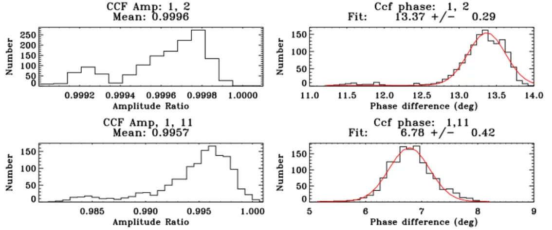
Fig. 1. Histogram of cross-correlation magnitude (left) and phase (right) estimated using receiving channels 1 and 2 (top) and 1 and 11
(bottom).
Fig. 2. Histogram of antenna phase differences.
2 The Buckland Park MF radar
The Buckland Park MF radar is located 35 km North of Ade-laide (34◦380S, 138◦290E), and operates at a frequency of
1.98 MHz. The antenna array consists of a 1-km diameter ar-ray of 89 individually accessible north–south and east–west aligned half-wave dipoles. The radar was upgraded between 1991 and 1995 (e.g. Reid et al., 1995), involving the refur-bishment of the entire antenna array and the commissioning of new transmitting and radar data acquisition (RDAS) sys-tems. The antenna array can now be used for transmission, enabling the BPMF to operate as a Doppler radar (e.g. Van-depeer and Reid, 1995). The flexibility of the radar allows one to use it for specialized experimental campaigns. Rou-tine spaced antenna observations are performed outside cam-paigns and maintenance periods.
The transmitting system consists of three 10-channel solid-state modules, each of which can be used as an individ-ual transmitter. Each transmitter channel consists of a power-amplification (PA) module, a phase control module (PCM), and a transmit-receive (T/R) switch. The PA modules for transmitters 1 and 2 each produce 2.5 kW nominal power, while those for transmitter 3 each produce 5 kW nominal power. The maximum total RMS peak envelope power for the system is, therefore, 100 kW. Each transmitter channel is connected to three dipoles of the antenna array, and these
dipoles can also be used for reception via the T/R switches. The PCMs allow the phase of the transmitted signal for each channel to be adjusted in 8.5◦increments, allowing the trans-mitter polar diagram to be steered off-zenith in any direction. The restriction to 8.5◦multiples produces negligible deteri-oration of the polar diagram in comparison to that obtained using exact phasing. Each transmitter produces Gaussian-shaped pulses with half-power full-width (HPFW) 14 µs , corresponding to a range resolution of ≈4 km HPFW. The duty cycle of each transmitter is approximately 0.2%.
The radar data acquisition system (RDAS) consists of 16 receiving channels, each comprising of a receiver and sig-nal processor. Each channel can be connected to individual dipoles or to groups of three dipoles, including those em-ployed for transmission via the T/R switches. The signal pro-cessors use 12-bit digitisation, which is increased to 16-bit upon coherent integration. The receiver bandwidths corre-sponds to a transmit HPFW of 2 km, which is half the trans-mit pulse duration. This bandwidth was chosen with the use of narrower transmit pulse widths and pulse coding in mind. Despite the bandwidth being nonoptimal, the combination of the wide beamwidth and narrow transmit beam minimises range smearing. The signal returns can be sampled at a 1- or 2-km range resolution.
The radar is controlled by a DOS-based (acquisition) PC which writes each individual raw data acquisition to file, and then transfers the file to a Linux (analysis) PC, where it is queued for analysis. The analysis is part of the “Analysis and Display suite” (ADS), a commercially avail-able package supplied by Atmospheric Radar Systems Pty. Ltd. (ATRAD). The ADS consists of analysis, postanaly-sis, and display modules. The analysis allows each raw data record to be analysed using a number of different tech-niques, and to be stored as spectra and covariance func-tions. The postanalysis allows incoherent averaging of spec-tra and covariance functions for further analysis, and pro-cessing of analysis products, such as hourly averages and the production of “plot files” of the analysed data results which can be sent to remote locations for display on web
pages via ftp. The latter functionality provides hourly up-dated latest result plots, as displayed at the web addresses http://www.physics.adelaide.edu.au/atmospheric and http:// www.atrad.com.au/results.html.
2.1 Receiver and antenna evaluation
Receiver characteristic differences can produce biased wind estimates when using the full correlation analysis (FCA). This bias is known as the “triangle size effect” (here-after TSE) (e.g. Golley and Rossiter, 1970; Meek, 1990; Holdsworth, 1999b), whereby the FCA “true” velocity de-creases with decreasing antenna spacing. Furthermore, phase differences between antenna systems combined for use by the FCA can also introduce the TSE (e.g. Holdsworth, 1999b). As a result, a number of tests were performed prior to routine analysis implementation, to investigate the contri-bution of these factors upon the FCA TSE, and for design of an optimal experimental configuration to reduce their effects. Receiver characteristic differences were determined as de-scribed by Golley and Rossiter (1970). A commercially available 8-way splitter was used to split the signal received by a single antenna into multiple receivers. Cross-correlation functions (CCFs) of the resulting signals were calculated. After interpolating across zero-lag to remove the effects of noise correlated between receiver channels (e.g. Briggs, 1984), the zero-lag CCF magnitudes were estimated to mea-sure the statistical similarity of the receiving channels, and the zero-lag CCF phases were estimated to measure the phase difference between channels. Examples of cross-correlation magnitude and phase histograms for two receiver pairs re-sulting from 200 2-min observations using all ranges with signal-to-noise ratios (SNRs) exceeding 10 dB are shown in Fig. 1. The mean of the correlation magnitude distribution for channels 1 and 2 is slightly less than unity, indicating slightly different receiver responses. This mean is typical of the values obtained comparing receivers 1–10 (and 11–16), which range from 0.999 to 1.0. In contrast, the means ob-tained using channels 1 and 11 are significantly smaller than unity. These means are typical of the values obtained com-paring receivers 1–10 with those from 11–16, which range from 0.990 to 0.995. This is due to minor design differ-ences between the two groups of receivers. A similar proce-dure was performed to compare the characteristics of the T/R switches, yielding correlations in the range of 0.999 to 1.0. Although a 1% departure from unity may seem a small and acceptable value, FCA velocity magnitude biases as large as 20% can occur for some combinations of antenna spac-ing and pattern scales appropriate for the Buckland Park MF radar. For this reason, it was decided to apply FCA using receivers 1 to 10 only.
Antenna system phase differences may be introduced by the antennas, baluns, or feeder cables. Antenna system phase differences were determined using zero-lag cross-covariance phases (or ZCCPs) obtained from several one-hour runs of 2-min observations using all ranges with SNRs exceeding 10 dB. The implicit assumption used is that the mean
an-gle of arrival (MAOA) for each record should be distributed about the zenith (e.g. Kudeki et al., 1990). Profiles of the ZC-CPs often exhibited significant offsets above 86 km, which can be attributed to the ionosphere. This behavior is consis-tently observed for the BPMF radar (K. J. Berkefeld, private communication). Similar offsets are observed for the Ur-bana MF radar by Thorsen et al. (1997). As a result, ZCCPs below 86 km were used to estimate the antenna phase ferences. The resulting mean ZCCP measure the phase dif-ferences introduced by the antenna system and the receiver. The receiver phase differences determined from the receiver characteristic tests described above are then subtracted to yield the phase differences introduced by the antenna sys-tem alone. The resulting distribution of antenna phase differ-ences with respect to an arbitrarily selected “good” antenna for each dipole orientation are shown in Fig. 2. The major-ity of the phase differences are less than 20◦. Time Domain
Reflectometry (TDR) measurements of antennas producing phase differences exceeding 20◦often indicated the presence of water in the air-cored coaxial cable. This behavior pro-duces the assymetry evident in the phase histogram as water acts to increase the electrical length of the cable, thereby pro-ducing large negative phase differences when compared with good antennas. Maintenance procedures are ongoing to im-prove such antennas and any other antenna related problems that may arise (e.g. Grant, 2004).
2.2 Antenna configuration and transmitter polar diagrams Simulations of the transmitter polar diagram obtained us-ing the entire BPMF antenna array for transmission suggest that randomly distributed phase differences less than 20◦ pro-duces negligible degradation of the polar diagram (e.g. Van-depeer, 1993). However, phase differences of this order can produce FCA TSE biases when groups of three antennas are combined for reception (e.g. Holdsworth, 1999b). As a re-sult, antennas with phase differences less than 20◦have been preferentially selected for transmission, while antennas with phase differences less than 10◦have been preferentially se-lected for reception.
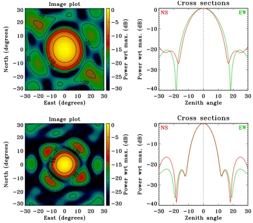
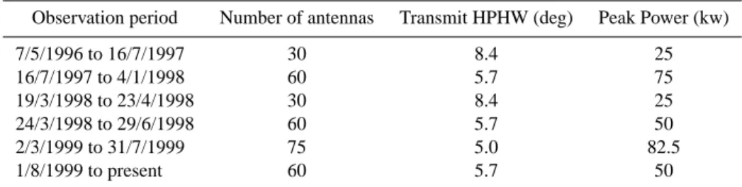
The antenna configuration has been modified throughout the observations as necessitated by antenna failures, reavail-ability of corrected antennas, transmitter availreavail-ability, and re-quirements to test different antenna configurations for partic-ular analyses. Transmission is performed using the north– south aligned antennas, producing a linearly polarized sig-nal. The number of transmit antennas and the total trans-mitter power for different observation periods are shown in Table 1. Except for a four month period in 1999, either 30 or 60 antennas have been used for transmission. The antenna configuration employed for the routine observations between 16 July 1997 and 4 January 1998 is shown in Fig. 3. The transmit polar diagrams obtained using the first 30 antennas (transmit modules 1 to 10) and all 60 antennas (transmit mod-ules 1 to 20) of this configuration are shown in Fig. 4. These polar diagrams are typical of those produced using 30 and 60 antennas throughout the observations, producing half-power
T20 T19 T18 T17 T16 T15 T12 T11 TR10 TR9 TR8 TR7 TR6 TR5 TR3 TR4 TR2 TR1 T14 T13 North/South Array North o 4 R16 R11 R12 R13 R14 R15 East/West array R10 R6 R7 R8 R9
Fig. 3. Antenna configuration employed for initial routine observations using the Buckland Park MF radar. Each vertical line on the
north/south array (left) represents a single north–south aligned antenna, while each horizontal line on the east/west array (right) represents a single east/west aligned antenna. The triangles denote the antennas used for observations, and the appropriate transmit channel. Antenna groups denoted TRi and Ti were connected to transmitter i. Antenna groups denoted TRi were connected to receiver i via T/R switch i.
Antenna groups denoted Ri were connected directly to receiver i. The filled circles denoted Ri were connected to receiver i for meteor
observations from March 2000.
Fig. 4. Polar diagrams employed for routine observations using the Buckland Park MF radar. The top plots show image (left) and
Table 1. Observation periods for routine Spaced Antenna (SA) analysis for the Buckland Park MF radar.
Observation period Number of antennas Transmit HPHW (deg) Peak Power (kw) 7/5/1996 to 16/7/1997 30 8.4 25 16/7/1997 to 4/1/1998 60 5.7 75 19/3/1998 to 23/4/1998 30 8.4 25 24/3/1998 to 29/6/1998 60 5.7 50 2/3/1999 to 31/7/1999 75 5.0 82.5 1/8/1999 to present 60 5.7 50
half-widths of 8.4◦and 5.7◦, respectively. Apart from a small degree of asymmetry, the polar diagrams otherwise show no undesirable features, despite the irregular antenna grid em-ployed. The maximum sidelobe levels are 13 dB below the peak power level.
Receivers 1 to 10 were initially connected to T/R switch outputs 1 to 10, and, therefore, to the north–south antenna groups 1 to 10. Receivers 11 to 16 were connected to the east–west aligned antennas corresponding to north–south an-tenna groups 1 to 6. Receiver 16 was connected to T/R switch 1 via an attenuator from 19 March 1998 onwards, to facilitate observations of descending E-region layers (e.g. Holdsworth et al., 2001), which generally saturate the receivers when used with the optimal receiver gain setting used for routine observations. Receivers 6 to 10 were connected directly to 5 east–west antennas from 14 September 2000 onwards, to provide an interferometer for meteor observations.
2.3 Complex gain difference estimation and correction Compensation for receiver channel complex gain differences is critical for accurate interferometric analyses, such as TDI, HDI, IDI and meteor analyses, and for accurate decompo-sition of the O- and E-mode signals for DAE analysis. Al-though the BPMF radar is capable of automated receiver cal-ibration (e.g. Reid et al., 1995), these measurements do not account for phase delays through the T/R switches, feeder cables and antennas. The receiver channel complex gain dif-ferences are, therefore, estimated using a receiver channel calibration (RCC) procedure. This procedure is typically per-formed monthly, using at least one day of daytime raw data archived by the routine analysis. Daytime data is preferred due to its higher SNR and lower interference level. The RCC is only applied using data with SNRs exceeding 10 dB, and is applied as follows.
The receiver channel amplitudes Ai are estimated by
cal-culating the zero-lag auto-covariance function magnitudes after interpolating over zero-lag to remove the effects of noise. The mean receiver channel amplitude ratios with re-spect to a selected reference receiver j are then estimated using Aij = Aj/Ai. The receiver channel phase differences
θij are estimated using the ZCCP with respect to a
refer-ence receiver channel j after interpolating over zero-lag to remove the effects of noise correlated between receiver
chan-nels. The mean receiver channel phase differences θij are
then estimated using the first moments from a Gaussian fit-ting, which is preferred to the mean as it is less influenced if the distribution is skewed or has significant tails. As de-scribed in Sect. 2.1, the implicit assumption used in this step of the RCC is that the MAOA over the observation period is on zenith. This is thought to be a valid assumption for the 8-h (or more) data sets used for the RCC. The complex gain correction used for multiplying each receiver channel i to correct for complex gain differences is then Aijexp −iθij.
Monthly estimated amplitude ratios and phase differences typically showed consistency to within the RMS values of the distributions on a month to month basis. The largest de-partures observed are usually associated with antenna system failures within a group of three antennas, and are typically of the order of 10% for amplitude ratios and 20◦for phase dif-ferences.
The RCC procedure is first performed for receivers 1 to 10, yielding the amplitude ratios and phase differences with respect to channel 1. For the same reasons described in Sect. 2.1, only phase differences below 86 km were used to estimate the receiver channel phase differences for receivers 1 to 10. The amplitude ratios were calculated using data from all ranges below 90 km. This limit was selected as receiver saturation can occur above 90 km, which can have significant effects on the estimated amplitude ratios.
The histogram procedures were then repeated for the crossed dipole receiver pairs 1–11, 2–12, 3–13, 4–14, 5– 15 and 6–16, using daytime data from ranges between 80 and 90 km. The upper limit was selected due to the possibil-ity of receiver saturation, which can have significant effects upon the estimated phase differences. The lower limit was selected as the O-mode signal above 80 km is significantly stronger than the E-mode signal during the day. The result-ing phase difference between each pair of cross-dipoles is therefore ≈ 90◦, allowing for the determination of the phase
difference between the two crossed dipoles. This allows for the amplitude and phase differences to be combined into a gain correction with respect to receiver 1, thereby providing the same complex gain reference for all receiver channels used in the DAE experiment. The range limiting procedure is essentially the same as suggested by Von Biel (1977) for the complex gain calibration for polarimetric observations.
Fig. 5. Examples of histograms of phase differences (left) and amplitude ratios (right) obtained by applying the RCC to daytime data from
between 4 and 9 April 2000. The red lines on the phase differences plots show the result of applying a Gaussian fit.
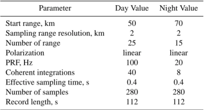
Table 2. Experimental parameters used for routine Spaced Antenna
(SA) analysis for the Buckland Park MF radar.
Parameter Day Value Night Value Start range, km 50 70 Sampling range resolution, km 2 2 Number of range 25 15 Polarization linear linear
PRF, Hz 100 20
Coherent integrations 40 8 Effective sampling time, s 0.4 0.4 Number of samples 280 280 Record length, s 112 112
An example of selected histograms of amplitude ratios and phase differences obtained on applying the RCC for daytime data between the 4 and 9 April 2000 is shown in Fig. 5. For routine observations from 14 September 2000 incorporating the meteor interferometer, the RCC for channels 6 to 10 was applied as a separate subset, with channel 6 used as the ref-erence channel.
2.4 Routine observations
Routine observations commenced 7 May 1996, using the pa-rameters shown in Table 2. Data acquisition is performed for 112 s, with the following 8 s used for transfer of the ≈1.5 Mb raw data files between the acquisition and analysis PCs. The only modification to these parameters has been the extension of the day (night) height range maximum to 158 (178) km from 19 March 1998, to allow for studies of descending total reflection layers. It is important to emphasize that each of the analyses described in Sects. 3 to 9 can be applied to each individual 2-min raw data set. Receiver calibration is applied prior to analysis. Data above 98 km is only analysed by the DBS analysis configured for the attenuated signal of receiver 16, and the meteor analysis. All routine observations outside
specialised Doppler campaigns use vertical beam transmis-sion.
3 Full correlation analysis
Full correlation analysis (FCA) (e.g. Briggs, 1984) has been applied throughout the observations, providing estimates of the dynamics and the spatial and temporal properties of the radiowave scatterers. The FCA has used antennas with simi-lar spacings to those connected to receivers 1, 2 and 3 (here-after “FCA-small”) shown in Fig. 3. On 2 March 1997 a second FCA analysis was implemented, using antennas with larger spacing, such as those connected to receivers 1, 6 and 9 (hereafter “FCA-large”). Preliminary FCA results are pre-sented by Holdsworth and Reid (1997) and Holdsworth et al. (2001). Further FCA results are presented in the accom-panying paper Holdsworth and Reid (2004).
The initial selection of a small spacing may be consid-ered unusual since FCA is known to be affected by the TSE. The motivation for using the smaller spacing was threefold. First, simulations suggest smaller spacings produce smaller measurement errors (e.g. Holdsworth, 1999b). This can be attributed to smaller spacings using cross-correlation func-tions with higher correlafunc-tions, and hence smaller correlation parameter errors. Second, smaller spacing reduces the oc-currence of cases where the antenna spacing exceeds the pat-tern scale. This results in low cross-correlation between the signals at each antenna, increasing the occurrence of spuri-ous velocity estimates due to the use of correlation param-eters with large errors, or correlation paramparam-eters estimated using incorrectly identified cross-correlation maxima. The FCA therefore applies criteria (e.g. Briggs, 1984) to reject low correlation maxima, large delay-times to cross-correlation maxima, and large normalised time-discrepancies (NTDs, the ratio of the sum of the delay times and sum of the absolute delay times), since NTD should be zero. Third, and perhaps most importantly, we felt confident that we had eliminated (or at worst minimised) all known TSE sources. It was later realised there were two further TSE sources that we
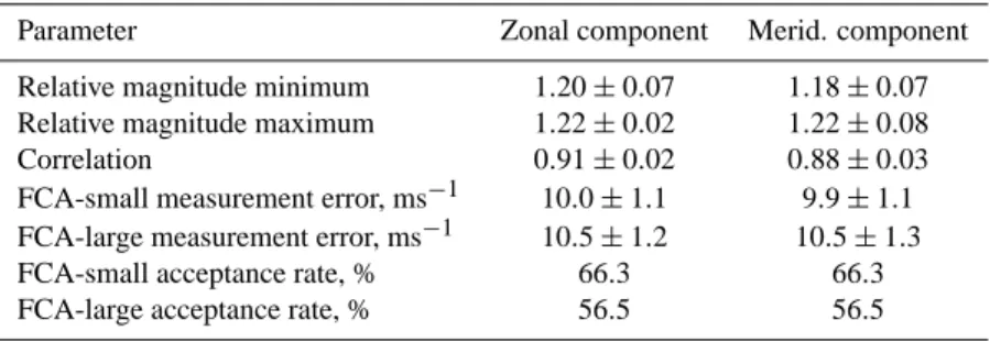
Table 3. Mean and standard deviation of daily relative magnitude minima and maxima, correlation, maximum measurement errors, and
acceptance rates for FCA-large relative to FCA-small from 2 March 1997 to 19 September 2003.
Parameter Zonal component Merid. component Relative magnitude minimum 1.20 ± 0.07 1.18 ± 0.07 Relative magnitude maximum 1.22 ± 0.02 1.22 ± 0.08 Correlation 0.91 ± 0.02 0.88 ± 0.03 FCA-small measurement error, ms−1 10.0 ± 1.1 9.9 ± 1.1 FCA-large measurement error, ms−1 10.5 ± 1.2 10.5 ± 1.3 FCA-small acceptance rate, % 66.3 66.3 FCA-large acceptance rate, % 56.5 56.5
Table 4. Mean and standard deviation of daily relative magnitude minima and maxima for “large-FCA” and “O-mode large-FCA” from 1
January 2001 to 25 July 2001.
Parameter Zonal component Merid. component Relative magnitude minimum 0.96 ± 0.02 0.96 ± 0.02 Relative magnitude maximum 0.96 ± 0.02 1.00 ± 0.02
could not eliminate: different configurations of combined an-tennas, and nonsimultaneous range sampling. The former is evident in Fig. 1, where antenna 3 has a different orientation from antennas 1 and 2. Selecting groups of antennas with identical orientations is unfeasible, given the dual require-ments of avoiding the use of bad antennas and maintaining satisfactory polar diagrams. The latter results from the dif-ferent feeder cable lengths used in the antenna array (e.g. Reid et al., 1995). Cable lengths of 0.5λ (4.5λ) feed the cen-ter (oucen-ter) antennas. The range gates sampled by the oucen-ter antennas are therefore 681 m lower than the center antennas. This represents a significant fraction (0.17) of the nominal transmit pulse half-power full-width (4 km) – although we note the different cable lengths will act to smear the trans-mitted pulse. Radar backscatter modeling (e.g. Holdsworth and Reid, 1995) of these effects suggested that the smaller spacing should produce an underestimation of at most 10%.
The FCA results have been used to investigate the TSE using the statistical comparison technique of Hocking et al. (2001), and the extension described by Holdsworth and Reid (2004). The daily mean relative magnitudes, correla-tions, “maximum” measurement errors and acceptance rates are shown in Table 3. The relative magnitudes indicate that FCA-small velocities are ≈20% smaller than FCA-large, in-dicating TSE. The FCA-small underestimation exceeds the expected value of 10%, suggesting a further unaccountable TSE source. The correlations are around 0.9, suggesting ex-cellent agreement. The estimated measurement errors for FCA-small are 5% smaller than those for FCA-large, which may only reflect the fact that the relative magnitudes are smaller. The FCA-large acceptance rate is 11% lower than FCA-small. The lower FCA-large acceptance rate results from large NTD and low cross-correlation maxima at heights
above 90 km, justifying the second motivation for our initial selection of the smaller spacing for FCA analysis.
Another source of TSE suggested by Holdsworth (1999b) is complex gain errors in the decomposition of the signals received by crossed dipoles into O- and E-mode circular po-larisation. Between 1 May 2001 and 25 July 2001 the FCA analysis was also applied to the O- and E-mode signals de-termined for the antennas used for FCA-large, as calculated for use in DAE analysis. The relative magnitude for O-mode winds in comparison with FCA-large are shown in Ta-ble 4, suggesting that the winds estimated using circularly polarised signals are slightly underestimated, which is con-sistent with the suggestions of Holdsworth (1999b). The BPMF routine analysis O- and E-mode signals are deter-mined post-receiver, which is not the case for most MF/HF radar systems. Regardless of the means by which circu-larly polarised signals are determined, there will be poten-tial sources of complex gain errors. The results of Table 4 suggest less biased velocity estimates may occur on apply-ing FCA usapply-ing linearly polarised antennas, as is the case for the BPMF routine analysis.
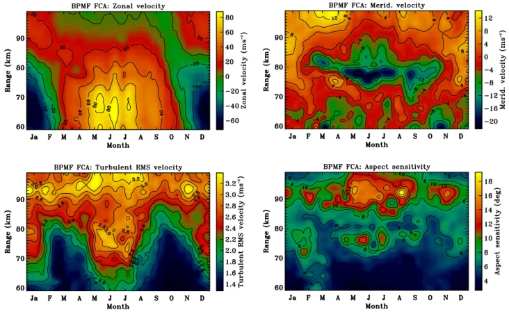
The annual variation of the FCA true velocity compo-nents, aspect sensitivity parameters (θs), and turbulent
ve-locities obtained using data from 07 July 1996 to 19 Septem-ber 2003 are shown in Fig. 6. These plots represent fort-nightly averages superposed into a single year: the 2-min data are averaged to produce hourly averages, which are then used to produce daily averages, which are then used to pro-duce fortnightly averages. FCA-small results are used until 2 March 1997, and FCA-large results thereafter. The aver-aging method used gives each hourly average equal weight in the daily average, and each daily average equal weight in the fortnightly average. This is preferred to a fortnightly
Fig. 6. Superposed annual variation of BPMF FCA parameters zonal velocity (top left), meridional velocity (top right), turbulent RMS
velocity (bottom left), and aspect sensitivity (bottom right).
average of the 2-min data, which would bias the averages towards the values obtained when the acceptance rates are largest. The zonal velocities above 84 km are predominantly eastwards except between mid-September to mid-November. The eastward/westward reversal height descends from 94 km in mid-September to 60 km in mid-November, a descent of approximately 0.56 km per day. Below 84 km the zonal ve-locities show the eastward winter jet and westward summer jet typically observed at mid-latitude stations (e.g. Manson et al., 1991). The winter jet shows greater variability than the summer jet, with peaks of 85 m s−1 at 68 km in late May, June and July, compared to a single summer jet peak of −68 m s−1. The winter peak times vary from year to year, but there are always two or three peaks each winter. The greater variability of the winter jet may be indicative of stratospheric warming (e.g. Manson et al., 1991), or possibly the failure of our averaging procedures to properly filter out planetary waves (e.g. Nakamura et al., 1996). The summer reversal height is around 84 to 85 km, consistent with pre-vious mid-latitude Southern Hemisphere observations (e.g. Manson et al., 1987). The meridional velocities are pre-dominantly northward above 70 km, with the exception of a strong southward peak extending from 82 km in March, to 77 km in June, and back up to 80 km in October, and weaker southward flows between the peak and 90 km in winter. Be-low 70 km the velocities are predominantly southward, and
show considerable variability. Turbulent velocities are es-timated as described by Briggs (1980), and increase with height. Solstice maxima and equinoctal minima are observed below 80 km. There is evidence of a maximum extending from 93 km in summer to above 98 km in winter. We at-tribute this to leakage from E-region total reflection, since harmonic analysis of BPMF turbulent velocities has been shown to yield turbulent velocities whose maxima peak at midday (e.g. Holdsworth et al., 2001). The aspect sensitiv-ity parameter θs is estimated using the “spatial correlation
technique” of Lesicar and Hocking (1992a), and increases with height, indicating less aspect sensitive scatter. The ex-ceptions are winter and summer maxima at 76 km, and weak maxima at all heights below 74 km in early March and Oc-tober. There is a weak minimum associated with the strong southward meridional velocity peak.
The above results are in qualitative agreement with the zonal and meridional velocities of Lesicar (1993) and the aspect sensitivities of Lesicar et al. (1992b), who presented a similar climatology using data from the previous BPMF radar, which used transmission on a separate 4-antenna dipole array with a large beam width, and an 8-bit data ac-quisition system. The main difference is that the veloci-ties presented in the current results are approximately 30% larger, and the aspect sensitivities are approximately 50% smaller. This is consistent with the hypothesis that the new
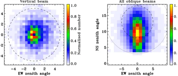
Fig. 7. Histograms of effective beam positions estimated during the 5-beam Doppler campaign July 1998. The left plot shows vertical beam,
while the right plot shows the combined results from the north, east, south and west beam directions, with the east, south and west beams results rotated to the north. The squares indicates the beam direction, and the diamonds indicates the zenith.
BPMF radar is less susceptible to TSE biases. The trans-mit beamwidths are considerably smaller than those usu-ally used for most MF/HF radar observations (20◦–40◦) (e.g. Vincent and Lesicar, 1991). FCA measurement er-rors have been shown to increase with decreasing beam-widths (e.g. Røyrvik, 1983; Kawano et al., 2002), as the resulting increase in the ground diffraction pattern scale in-creases the errors in the correlation parameters used in the analysis. However, the measurement errors in the corre-lation parameters decrease with increasing SNR. Since in-creasing the flux of power directed vertically (from which the strongest returns emanate) increases SNR, it is expected that any increase in measurement errors due to pattern scale increases are more than compensated for. The increased SNR also extends the lowest observation range – Holdsworth and Reid (1997) show regular winter daylight velocity estimates down to 52 km, considerably lower than that achieved using previous BPMF radar systems.
4 Differential absorption experiment
The Differential absorption experiment (DAE) (e.g. Gard-ner and Pawsey, 1953) was implemented in August 1996 for the estimation of electron densities and collision frequencies. Receiver outputs 1 to 5 are combined with receiver outputs 11 to 15 to form five pairs of ordinary (O-mode) and ex-traordinary (E-mode) signals. The five O-mode signals are combined to produce the O-mode signal used for analysis, and the five E-mode signals similarly are combined to pro-duce the E-mode signal. Detailed information regarding the BPMF DAE analysis and electron density estimates are pre-sented by Holdsworth et al. (2002), while collision frequency estimates are presented by Vuthaluru et al. (2002).
Table 5. Mean and standard deviation of daily relative magnitude
minima and maxima, correlation, maximum measurement errors, and acceptance rates for SCA relative to FCA-small from 18 Octo-ber 1996 to 1 May 1997.
Parameter Zonal component Merid. component Relative magnitude minimum 1.24 ± 0.08 1.30 ± 0.05 Relative magnitude maximum 1.32 ± 0.03 1.34 ± 0.04 Correlation 0.95 ± 0.01 0.91 ± 0.03 SCA measurement error, ms−1 10.7 ± 0.8 10.8 ± 0.7 FCA measurement error, ms−1 9.7 ± 0.4 9.7 ± 0.5 SCA acceptance rate, % 30.7 30.7 FCA acceptance rate, % 60.3 60.3
5 Spatial correlation analysis
The revised spatial correlation analysis (SCA) (e.g. Holdsworth, 1999a) was implemented on 18 October 1996. The SCA was applied to the square of receiving channels 1, 2, 4 and 5 shown in Fig. 3. Antenna degradation through-out the observations made maintaining the square configu-ration difficult, and SCA was discontinued on 1 May 1997. The major motivation for investigating SCA was that previ-ous implementation illustrated that the velocities compared well with FCA velocities estimated for large antenna spac-ings (e.g. Golley and Rossiter, 1970), suggesting a less biased velocity estimate than FCA, which is subject to the TSE. A detailed examination of the performance of the SCA is con-sidered beyond the scope of this paper, although some as-pects of the analysis performance are discussed below.
Table 5 shows the results of applying the aforementioned statistical comparison technique to the SCA and FCA-small velocities estimated from 18 October 1996 to 1 May 1997. The relative magnitude maxima suggest the SCA velocities are approximately 30% larger than the FCA-small
veloci-Table 6. Mean and standard deviation of daily relative magnitude
minima and maxima for HDI relative to DBS from 18 June 1998 to 29 June 1998.
Parameter Zonal component Merid. component Relative magnitude minimum 1.19 ± 0.06 1.36 ± 0.04 Relative magnitude maximum 1.52 ± 0.01 1.38 ± 0.06
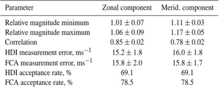
Table 7. Mean and standard deviation of daily relative magnitude
minima and maxima, correlation, maximum measurement errors, and acceptance rates for HDI relative to FCA-large from 18 June 1998 to 29 June 1998.
Parameter Zonal component Merid. component Relative magnitude minimum 1.01 ± 0.07 1.11 ± 0.03 Relative magnitude maximum 1.06 ± 0.09 1.17 ± 0.05 Correlation 0.85 ± 0.02 0.78 ± 0.02 HDI measurement error, ms−1 15.2 ± 1.8 16.0 ± 1.8 FCA measurement error, ms−1 15.8 ± 2.0 15.8 ± 1.7 HDI acceptance rate, % 69.1 69.1 FCA acceptance rate, % 78.5 78.5
ties, which, as described above, are underestimated due to the TSE. The correlations exceed 0.9, suggesting excellent agreement. The estimated measurement errors for the FCA-small are FCA-smaller than those for SCA. However, as per the FCA comparisons in Sect. 3, we cannot conclusively deter-mine the actual relative measurement errors, since the es-timated relative measurement errors are influenced by the relative magnitudes. The acceptance rate for the SCA is approximately half that of FCA-small. The majority of extra rejections for the SCA are associated with a criterion requir-ing the cross-correlations for antenna pairs with the same ori-entation (e.g. 14 and 25 in Fig. 3) agree to within 20% (e.g. Holdsworth, 1999a). This represents a test for spatial homo-geneity of the ground diffraction pattern, which is necessary for successful SCA velocity estimation. Investigation of both MF/HF and tropospheric VHF SCA analysed data shows this criterion occurs most frequently for either isotropic scatter (i.e. ground diffraction scales smaller than the antenna spac-ing) or specular scatter. It results in 23% of the rejections above 90 km for the BPMF data. The high occurrence may be exacerbated by the effects of unequal cable lengths, which can reduce cross-correlations as described in Sect. 3. Further work is intended to loosen this criteria without producing spurious velocity estimates, and to evaluate the implications of the apparent spatial inhomogeneity this criterion suggests upon the FCA.
For completeness we briefly mention that the SCA anal-ysis has also been applied using the Wakkanai MF radar (e.g. Hocke and Igarashi, 1997). This analysis differs from the BPMF analysis only in the application to antennas ar-ranged in a “Y” configuration. Application of the statis-tical comparison technique to this data yields correlations,
measurement errors and acceptance rates show similarity to the values shown in Table 4. The relative ratios of the SCA to FCA velocities are approximately 1.05, suggesting that the Wakkanai FCA velocities are less biased than the BPMF FCA-large velocities. This is most probably due to the Wakkanai MF radar using a smaller transmit array than the BPMF radar, such that the receive antennas are a better match to the pattern scale, and the FCA is therefore less in-fluenced by TSE biases.
6 Beam steering
The Doppler beam steering (DBS) and hybrid Doppler in-terferometry (HDI) techniques were implemented in April 1997. DBS is applied by combining all receiving channels to form a receive beam in the same direction as the transmit beam and applying standard Doppler analysis (e.g. Wood-man and Guillen, 1974), to estimate radial velocity, spec-tral width, SNR and power. HDI uses post-statistics steering (PSS) (e.g. Kudeki and Woodman, 1990), to estimate the “ef-fective beam position” (EBP), allowing correction for (and estimation of) aspect sensitivity, which reduces the mean an-gular position of backscatter for off-zenith beam directions (e.g. R¨ottger, 1981). PSS is used to form a receive beam which is steered through a grid of beam directions. The power for each beam direction is determined, and the EBP is found by applying a 2-D Gaussian to estimate the direc-tion of maximum power. The receive beam is then resteered in the direction of the EBP, and the standard DBS param-eters are estimated. The use of PSS allows the EBP to be determined more accurately (and to lower SNRs) than using the MAOA, since it uses combined receiver outputs, while the MAOA is estimated by cross-correlating single receiver outputs. The term “hybrid Doppler interferometry” is used as the technique is a hybrid of Doppler and interferometric techniques, and is used in preference to “time domain in-terferometry” (TDI) (e.g. Vandepeer and Reid, 1995), since the analysis can be applied in the time or frequency domain. For BPMF observations the technique is applied in the time-domain, since spectra obtained for mesospheric and lower thermospheric MF/HF radar observations are often irregular and non-Gaussian. Although HDI and DBS analyses are in-tended for off-vertical transmission, the vertical beam used throughout routine observations allows for HDI estimated MAOAs and radial velocities to be used for TDI, allowing dynamics estimates for durations ranging from hours (e.g. Berkefeld, 1994) to months (e.g. Thorsen et al., 1997).
HDI and DBS analyses were only intermittently applied throughout the routine observations until 19 March 1998, when DBS analysis was configured for application to re-ceiver 16 for investigations of E-region descending layers. However, both analyses have been applied during several 5-beam Doppler campaigns for momentum flux estimation us-ing the dual-beam technique (e.g. Vincent and Reid, 1983). The EBPs estimated for all four oblique from 18 to 29 June 1998 are shown in Fig. 7. The most common EBP is 9.5◦,
yielding twice as many estimates as at the actual beam po-sition of 13◦. Table 6 shows the statistical comparison of
the DBS and HDI techniques for 18 to 29 June 1998, while Table 7 shows the comparison for the HDI and FCA-large ve-locities. The HDI and FCA velocities show good agreement, while the standard Doppler velocities are underestimated due to the EBP being closer to zenith. A more extensive evalu-ation of the 5-beam Doppler results will be presented in a future paper.
7 Meteor analysis
Following the successful BPMF meteor observations of Tsut-sumi et al. (1999), the Atrad VHF meteor analysis software (e.g. Holdsworth et al., 2004) was modified for BPMF rou-tine analysis, and was implemented on 8 April 1999. While the background signal for VHF radars is usually noise, the background signal for MF/HF radars is often coherent iono-spheric echoes. Application for MF meteor studies therefore required the development of an improved detection algorithm and criteria to reject ionospheric echoes. The meteor analysis initially used receivers 1 to 5, requiring a complicated AOA estimation procedure which was often unsuccessful in re-solving AOA ambiguities. Analysis from 14 September 2000 was applied using the interferometer formed by receivers 6 to 10 shown in Fig. 3, allowing for application of a technique similar to that described by Jones et al. (1998), which greatly reduced AOA ambiguities. Since the smallest effective spac-ing attainable is 0.6λ the maximum unambiguous zenith an-gle is 56.4◦. In most cases AOAs ambiguities can be resolved
by calculating the echo height for each AOA candidate and assuming limits (70 to 140 km) for valid meteor heights.
Figure 8 shows distributions of various meteor parameters, while Fig. 9 shows comparison of superposed meteor and FCA zonal winds for March 2003. A total of 8924 meteors (average 287 per day) were observed. The height distribu-tion peaks at 105 km and extends from 80 to 140 km, com-paring well with previous BPMF meteor observations (e.g. Brown, 1976; Olsson Steel and Elford, 1987). The upper limit exceeds that of Tsutsumi et al. (1999) by 20 km, which we attribute to the larger sampling range maximum used in the present study (178 km compared to 148 km). The diurnal distribution shows very few meteors during the day. Those obtained are limited to heights below 100 km due to E-layer total reflection, as is evident from the zonal winds shown in Fig. 9. The AOAs are mostly located within 60◦ of zenith,
with the largest zenith angle being 66◦. Less than 6% of the
AOAs are detected within the main lobe of the transmit polar diagram. The decay time distribution shows good agreement with theoretical estimates obtained using CIRA86 tempera-ture and pressure estimates (e.g. Cervera and Reid, 2000), although they show significantly more scatter than typical VHF distributions (e.g. Hocking et al., 1997; Cervera and Reid, 2000). This appears to be typical of 2–10 MHz meteor observations (e.g. Tsutsumi et al., 1999; MacDougall and Li, 2001), and may result from the effects of wind shears (e.g.
Tsutsumi et al., 1999) and turbulence (e.g. Brown, 1976), which have potentially more influence on MF/HF decay time estimates due to the longer echo durations. The velocity comparison show qualitative agreement in the overlapping height range, with the meteor estimates being larger. A sim-ilar result was observed by Cervera and Reid (1995), who found MF/FCA winds underestimated meteor wind compar-isons above 90 km. The FCA and meteor velocities clearly exhibit a diurnal variation, as expected at Adelaide in March, where the diurnal tide maximises (e.g. Holdsworth et al., 2001).
It should be stressed that the meteor analysis is applied to data collected using experimental parameters optimal for at-mospheric observations, and that no parameter modification has been made to facilitate the meteor analysis. In particu-lar, the effective sampling time of 0.4 s reduces the ability to detect short-lived meteors at heights above 110 km. Thus, al-though the number of meteors detected is considerable lower than VHF meteor radars, Figs. 8 and 9 suggest useful obser-vations can be made.
8 Imaging Doppler interferometry
Imaging Doppler interferometry (IDI) analysis (e.g. Adams et al., 1986) was introduced in August 2000, providing com-parative dynamical estimates for the FCA. The fundamen-tal assumption of IDI is that the phase information at each Doppler frequency results from a single discrete scattering location. Although some authors apply criteria to reject Doppler frequencies where this does not appear to be the case from the analysis (e.g. Adams et al., 1986; Meek and Manson, 1987). Franke et al. (1990) have shown comparable velocity estimates to the FCA are obtained without the use of rejection criteria. The IDI analysis implemented for the BPMF closely follows that of Franke et al. (1990), using an-tennas with similar spacings to those connected to receivers 1, 2 and 3 shown in Fig. 3. This analysis and the results are described in the accompanying paper by Holdsworth and Reid (2004).
9 Summary and future work
The routine analysis scheme used by the new Buckland Park MF radar has been presented. The raw data collected is si-multaneously analysed by a number of different analyses for the estimation of winds, electron densities, and meteor pa-rameters.
Figure 10 represents an attempt to compare the relative velocities shown in Tables 3 to 7 and the IDI estimates of Holdsworth and Reid (2004) to a common reference, the FCA-large velocities. As this comparison includes veloc-ities estimated from different analyses applied over differ-ent observation periods and using differdiffer-ent antenna config-urations, it should be interpreted with some caution. The results suggest that the HDI and SCA velocities show rela-tively good agreement, while the DBS velocities are
under-Fig. 8. Meteor distributions for March 2003: height (top left), time (top right), decay times (bottom left) and angle of arrival (bottom right).
The dashed lines in the angle of arrival plot indicate zenith angles of 20◦,40◦,and 60◦. The solid line in the decay time plot indicates the theoretical value estimated using CIRA temperature and pressure.
Fig. 9. Superposed velocities estimated using meteor (top) and full
correlation analysis (bottom) for March 2003.
estimated. This underestimation results from EBP being bi-ased towards zenith. HDI is able to compensate for this ef-fect by estimating the EBP, and, therefore, provides a less biased velocity estimate than DBS. HDI is a relatively new technique, and there has been little investigation into
poten-Fig. 10. Relative velocity magnitudes for various analyses with
re-spect to ”FCA-large”. The red and blue bars denote the range of ratios for the zonal and meridional components, respectively.
tial biases. The SCA is expected to be independent of TSE biases, and is, therefore, expected to be a less biased veloc-ity estimate than the FCA. Given that SCA and HDI are in-dependent techniques whose relative magnitudes show good
agreement and appear less biased than FCA or DBS, we feel reasonably confident that both may well be unbiased – al-though further investigations will be needed to confirm this is the case. On the other hand, the FCA is susceptible to the TSE, as reflected in the FCA-large velocities being approxi-mately 5–10% smaller than the SCA and HDI velocities. The IDI relative velocity magnitudes also show good agreement with the SCA and HDI velocities, despite predictions that the IDI velocity is overestimated in the volume scatter sit-uation. Holdsworth and Reid (2004) suggest the agreement is due to a radial velocity threshold applied in the analysis, and that abolishing this threshold produces the volume scat-ter predicted overestimation.
There are a number of improvements and revised analy-ses intended to be implemented into the BPMF radar in the near future. One improvement involves the replacement of the DOS-based acquisition PC with a Linux PC. This will remove data transfer rate restrictions, allowing the radar to be operated with extended range maxima and reduced (or no) coherent integration. This will benefit meteor observa-tions, with the former allowing meteors to be detected at greater ranges, and the latter improving the detectability of short-lived meteors, and allow the application of meteoroid velocity estimation techniques reliant on short effective sam-pling times (e.g. Cervera et al., 1997; Grant, 2004). The former may also allow improved interference rejection (e.g. Hocking, 1997b). One revised analysis we intend to im-plement is polarimetric DAE analysis (e.g. von Biel, 1977), which will allow daytime electron densities to be calculated to greater heights by decomposing the signals received on crossed dipoles into “elliptical” polarisation, rather than cir-cular polarisation as used for simplicity in the current DAE analysis. The radar will continue to be used to test new anal-yses. A number of variations of the standard FCA are cur-rently being tested, and preliminary results from one such analysis are described in Holdsworth and Reid (2004).
Acknowledgements. Thanks to Rupa Vuthaluru, Masaki Tsutsumi,
Bob Vincent, Karen Berkefeld, Stephen Grant and Jonathan Woithe for their contributions to the work described in this paper, and Alex Didenko, Lesley Rutherford, Simon Ludbhorz, Stan Woithe and Malcolm Kirby for technical support. The Buckland Park MF radar was supported by Australian Research Council grants A69031462 and A69231890.
Topical Editor U.-P. Hoppe thanks two referees for their help in evaluating this paper.
References
Adams, G. W., Brosnahan, J. W., Walden, D. C., and Nerney, S. F.: Mesospheric observations using a 2.66 MHz radar as an imaging Doppler interferometer, J. Geophys. Res., 91, 1671–1683, 1986. Berkefeld, K. J.: Time domain interferometry wind estimations at mesospheric heights, Honours thesis, Univ. of Adelaide, Ade-laide, Aust., 1994.
Briggs, B. H.: Radar observations of atmospheric winds and tur-bulence: A comparison of techniques, J. Atmos. Terr. Phys., 42, 823–833, 1980.
Briggs, B. H.: The analysis of spaced sensor records by correlation techniques, in Handbook for MAP, SCOSTEP Secr., Univ. of Ill., Urbana, 13, 166–186, 1984.
Briggs, B. H.: On radar interferometric techniques in the situation of volume scatter, Radio Sci., 30, 1, 109–114, 1995.
Briggs, B. H., Elford, W. G., Felgate, D. G., Golley, M. G., Rossiter, D. E., and Smith, J. W.: Buckland Park aerial array, Nature, 223, 5213, 1321–1325, 1969.
Brosnahan, J. W. and Adams, G. W.: The MAPSTAR Imaging Doppler Interferometer: Description and first results, J. Atmos. Terr. Phys., 55, 203–228, 1993.
Brown, N.: Radio echoes from meteor trains at a radio frequency of 1.98 MHz, J. Atmos. Terr. Phys., 33(1), 83-87, 1976.
Cervera, M. A. and Reid, I. M.: Comparison of simultaneous wind measurements using colocated VHF meteor and MF spaced an-tenna radar systems, Radio Science, 30, 4, 1245–1261, 1995. Cervera, M. A. and Reid, I. M.: Comparison of atmospheric
param-eters derived from meteor observations with CIRA, Radio Sci-ence, 35, 3, 833–843, 2000.
Cervera, M. A., Elford, W. G., and Steel, D. I.: A new method for the measurement of meteor speeds: The pre-t0phase technique
Radio Science, 32, 2, 805–816, 1997.
Franke, P. M., Thorsen, D., Champion, M., Franke, S. J., and Kudeki, E.: Comparisons of time- and frequency-domain tech-niques for wind velocity estimation using multiple-receiver MF radar data, Geophys. Res. Lett., 17, 2193–2196, 1990.
Gardner, F. F. and Pawsey, J. L.: Study of the ionospheric D-region using partial reflections, J. Atmos. Terr. Phys., 3, 321–344, 1953. Golley, M. G. and Rossiter, D. E.: Some tests of methods of analysis of ionospheric drift records using an array of 89 aerials, J. Atmos. Terr. Phys., 32, 1215–1233, 1970.
Grant, S. I.: Radar studies of meteors at medium frequency, Ph. D. thesis, University of Adelaide, Australia, 2004.
Hocke, K. and Igarashi, K.: Variability and anisotropy of meso-spheric wind spectra Geophys. Res. Lett., 24, 22, 2725–2728, 1997.
Hocking, W. K.: System design, signal-processing procedures, and preliminary results for Canadian (London, Ontario) VHF atmo-spheric radar Radio Sci, 32, 2, 687–706, 1997a.
Hocking, W. K.: Recent advances in radar instrumentation and techniques for studies of the mesosphere, stratosphere and tro-posphere, Radio Sci, 32, 6, 2241–2270, 1997b.
Hocking, W. K., Thayaparan, T., Franke, S. J.: Method for statistical comparison of geophysical data by multiple instruments which have differing accuracies, Adv. Space Res., 27(6-7), 1089–1098, 2001.
Hocking, W. K., Thayaparan, T., and Jones, J.: Meteor decay times and their use in determining a diagnostic mesospheric temperature-pressure parameter: methodology and one year of data Geophys. Res. Lett., 24, 23, 2977–2980, 1997.
Holdsworth, D. A.: Spatial correlation analysis revisited: Theory, and application using “radar backscatter model” data, Radio Sci., 34, 3, 629–642, 1999a.
Holdsworth, D. A.: The influence of instrumental effects upon the full correlation analysis, Radio Sci., 34, 3, 643–656, 1999b. Holdsworth, D. A. and Reid, I. M.: A simple model of atmospheric
radar backscatter: Description and application to the full corre-lation analysis of spaced antenna data, Radio Sci., 30, 4, 1263– 1280, 1995a.
Holdsworth, D. A. and Reid, I. M.: Spaced antenna analysis of at-mospheric radar backscatter model data, Radio Sci., 30, 5, 1417– 1433, 1995b.
Holdsworth, D. A. and Reid, I. M.: An investigation of biases in the full correlation analysis technique, Adv. Space Res., 20, 6, 1269–1272, 1997.
Holdsworth, D. A. and Reid, I. M.: The Buckland Park meteor radar – description and initial results, Proceedings “Workshop on Ap-plications of Radio Science”, Leura, Australia, 2002.
Holdsworth, D. A. and Reid, I. M.: Comparisons of full correlation analysis (FCA) and imaging Doppler interferometry (IDI) winds using the Buckland Park MF radar, Ann. Geophys., 11, 3829– 3842 , 2004.
Holdsworth, D. A., Vincent, R. A., and Reid, I. M.: Mesospheric turbulent velocity estimation using the Buckland Park MF radar, Ann. Geophys., 19, 8, 1007–1017, 2001.
Holdsworth, D. A., Vuthaluru, R., Vincent, R. A., and Reid, I. M.: Differential absorption measurements of mesospheric and lower thermospheric electron densities using the Buckland Park MF radar, J. Atmos. Solar Terr. Phys, 64, 18, 2029–2042, 2002. Jones, J., Webster, A. W., and Hocking, W. K.: An improved
inter-ferometer design for use with meteor radars, Radio Science, 33, 1, 55–66, 1998.
Kawano, N., Tahara, Y., and Fukao, S.: Comparison of wind estima-tion errors for the spaced antenna technique: A case study for the MU radar, Radio Sci., 37, 5, doi:10.1029/2000RS002533, 2002. Kudeki, E. and Woodman, R. F.: A post-statistics steering technique for MST radar applications, Radio Sci., 25, 4, 591–594, 1990. Kudeki, E., S¨ur¨uc¨u, F., and Woodman, R. F.: Mesospheric wind
and aspect sensitivity measurements at Jicamarca using radar in-terferometry and poststatistics steering techniques, Radio Sci., 25, 4, 595–612, 1990.
Lesicar, D.: Study of the structure of partial reflection radar scat-terers and their application in atmospheric measurements, Ph.D. thesis, University of Adelaide, Adelaide, 1993.
Lesicar, D. and Hocking, W. K.: Studies of the seasonal behavior of the shape of mesospheric scatterers using a 1.98 MHz radar, J. Atmos. Terr. Phys., 54, 295–309, 1992a.
Lesicar, D., Hocking, W. K., and Vincent, R. A.: Comparative stud-ies of scatterers observed by MF radars in the polar summer hemisphere mesosphere, J. Geophys. Res., 97, 887–897, 1992b. MacDougall, J. W. and Li, X.: Meteor observations with a modern
digital ionosonde, J. Atmos. Terr. Phys., 63, 2–3, 135–141, 2001. Manson, A. H., Meek, C. E., Massebeuf, M., Fellous, J. L., Elford, W. G. Vincent, R. A., Craig, R. L., Roper, R. G., Avery, S. K., Balsley, B. B., Fraser, G. J, Smith, M. J., Clark, R. R., Kato, S., and Tsuda, T.: Mean winds in the upper atmosphere (70–110 km) from the global radar network: comparisons with CIRA 72, and new rocket and satellite data, Adv. Space Res, 7, 10 143–10 153, 1987.
Manson, A. H., Meek, C. E., Fleming, E., Chandra, S., Vincent, R. A., Phillips, A., Avery, S. K., Fraser, G. J, Smith, M. J., Fellous, J. L., and Massebeuf, M.: Comparisons between satellite derived gradient winds and radar derived winds from CIRA-86, J. Atmos. Sci., 48, 3, 411–428, 1991.
Meek, C. E.: Triangle size effect in spaced antenna wind measure-ments, Radio Sci., 25, 4, 641–648, 1990.
Meek, C. E. and Manson, A. H.: Mesospheric motions observed by simultaneous Medium-frequency Interferometer and Spaced Antenna experiments, J. Geophys. Res., 92, 5627–5639, 1987. Nakamura, T., Tsuda, T., and Fukao, S.: Mean winds at 60–90 km
observed with the MU radar (35◦N), J. Atmos. Terr. Phys., 58, 6, 655–660, 1996.
Olsson Steel, D. I. and Elford, W. G.: The height distribution of radio meteors: observations at 2 MHz, J. Atmos. Terr. Phys., 49, 243–258, 1987.
Reid, I. M., Vandepeer, B. G. W., Dillon, S. C., and Fuller, B. M.: The new Adelaide medium frequency Doppler radar, Radio Sci., 30, 4, 1177–1189, 1995.
Røyrvik, O.: Spaced antenna drift at Jicamarca, mesospheric mea-surements, Radio Sci., 18, 3, 461–476, 1983.
Thorsen, D., Franke, S. J., and Kudeki, E.: A new approach to MF radar interferometry for estimating mean winds and momentum flux, Radio Sci., 32, 2, 707–726, 1997.
Tsutsumi, M., Holdsworth, D. A., Nakamura, T., and Reid, I. M.: Meteor observations with an MF radar, Earth, Planets, Space, 51, 691–699, 1999.
Vandepeer, B. G. W.: A new MF Doppler radar for upper at-mospheric research, Ph.D. thesis, Univ. of Adelaide, Adelaide, Aust., 1993.
Vandepeer, B. G. W. and Reid, I. M.: Some preliminary results ob-tained with the new Adelaide MF Doppler radar, Radio Sci., 30, 4, 1191–1203, 1995.
Vincent, R. A. and Reid, I. M.: HF radar measurements of meso-spheric gravity wave momentum fluxes, J. Atmos. Sci., 40, 1321–1333, 1983.
Vincent, R. A. and Lesicar, D.: Dynamics of the equatorial meso-sphere: First results with a new generation partial reflection radar, Geophys. Res. Lett., 18, 5, 825–828, 1991.
Vincent, R. A., May, P. T., Hocking, W. K., Elford, W. G., Candy, B. H., and Briggs, B. H.: First results with the Adelaide VHF radar: Spaced antenna studies of tropospheric winds, J. Atmos. Terr. Phys., 49, 353–366, 1987.
von Biel, H. A.: The phase switched correlation polarimeter – a new approach to the partial reflection experiment, J. Atmos. Terr. Phys., 39, 769–778, 1977.
Vuthaluru, R., Vincent, R. A., Holdsworth, D. A., and Reid, I. M.: Collision frequencies in the D-region, J. Atmos. Solar Terr. Phys, 64, 18, 2043–2054, 2002.
Woodman, R. F. and Guillen, A.: Radar observations of winds and turbulence in stratosphere and mesosphere, J. Atmos. Sci., 31, 493–505, 1974.