HAL Id: hal-00317795
https://hal.archives-ouvertes.fr/hal-00317795
Submitted on 22 Dec 2004
HAL is a multi-disciplinary open access
archive for the deposit and dissemination of
sci-entific research documents, whether they are
pub-lished or not. The documents may come from
teaching and research institutions in France or
abroad, or from public or private research centers.
L’archive ouverte pluridisciplinaire HAL, est
destinée au dépôt et à la diffusion de documents
scientifiques de niveau recherche, publiés ou non,
émanant des établissements d’enseignement et de
recherche français ou étrangers, des laboratoires
publics ou privés.
Coordinated polar spacecraft, geosynchronous
spacecraft, and ground-based observations of
magnetopause processes and their coupling to the
ionosphere
G. Le, S.-H. Chen, Yunlin Jacques Zheng, C. T. Russell, J. A. Slavin, C.
Huang, S. M. Petrinec, T. E. Moore, J. Samson, H. J. Singer, et al.
To cite this version:
G. Le, S.-H. Chen, Yunlin Jacques Zheng, C. T. Russell, J. A. Slavin, et al.. Coordinated polar
spacecraft, geosynchronous spacecraft, and ground-based observations of magnetopause processes and
their coupling to the ionosphere. Annales Geophysicae, European Geosciences Union, 2004, 22 (12),
pp.4329-4350. �hal-00317795�
Annales Geophysicae (2004) 22: 4329–4350 SRef-ID: 1432-0576/ag/2004-22-4329 © European Geosciences Union 2004
Annales
Geophysicae
Coordinated polar spacecraft, geosynchronous spacecraft, and
ground-based observations of magnetopause processes and their
coupling to the ionosphere
G. Le1, S.-H. Chen2, Y. Zheng3, C. T. Russell4, J. A. Slavin1, C. Huang5, S. M. Petrinec6, T. E. Moore1, J. Samson7, H. J. Singer8, and K. Yumoto9
1Laboratory for Extraterrestrial Physics, NASA Goddard Space Flight Center, Greenbelt, MD 20771, USA
2Universities Space Research Association, NASA Goddard Space Flight Center, Greenbelt, MD 20771, USA
3NRC, NASA Goddard Space Flight Center, Greenbelt, MD 20771, USA
4Institute of Geophysics and Planetary Physics, University of California, Los Angeles, CA 90095-1567, USA
5MIT Haystack Observatory, Westford, MA 01886, USA
6Space Physics Laboratory, Lockheed Martin Advanced Technology Center, Palo Alto, CA 94304-1187, USA
7Department of Physics, University of Alberta, Edmonton, Alberta, T6G 2E1, Canada
8NOAA Space Environment Center, Boulder, CO 80305, USA
9Space Environment Research Center, Kyushu University, 6-10-1, Hakozaki, Higashi-ku, Fukuoka 812-8581, Japan
Received: 27 April 2004 – Revised: 28 September 2004 – Accepted: 6 October 2004 – Published: 22 December 2004
Abstract. In this paper, we present in-situ observations of processes occurring at the magnetopause and vicinity, including surface waves, oscillatory magnetospheric field lines, and flux transfer events, and coordinated observa-tions at geosynchronous orbit by the GOES spacecraft, and
on the ground by CANOPUS and 210◦Magnetic Meridian
(210 MM) magnetometer arrays. On 7 February 2002, dur-ing a high-speed solar wind stream, the Polar spacecraft was skimming the magnetopause in a post-noon meridian plane for ∼3 h. During this interval, it made two short excursions and a few partial crossings into the magnetosheath and ob-served quasi-periodic cold ion bursts in the region adjacent to the magnetopause current layer. The multiple magnetopause crossings, as well as the velocity of the cold ion bursts, indi-cate that the magnetopause was oscillating with an ∼6-min period. Simultaneous observations of Pc5 waves at geosyn-chronous orbit by the GOES spacecraft and on the ground by the CANOPUS magnetometer array reveal that these mag-netospheric pulsations were forced oscillations of magnetic field lines directly driven by the magnetopause oscillations. The magnetospheric pulsations occurred only in a limited longitudinal region in the post-noon dayside sector, and were not a global phenomenon, as one would expect for global field line resonance. Thus, the magnetopause oscillations at the source were also limited to a localized region span-ning ∼4 h in local time. These observations suggest that it is unlikely that the Kelvin-Helmholz instability and/or fluc-tuations in the solar wind dynamic pressure were the direct driving mechanisms for the observed boundary oscillations.
Correspondence to: G. Le
Instead, the likely mechanism for the localized boundary os-cillations was pulsed reconnection at the magnetopause oc-curring along the X-line extending over the same 4-h re-gion. The Pc5 band pressure fluctuations commonly seen in high-speed solar wind streams may modulate the recon-nection rate as an indirect cause of the observed Pc5 pul-sations. During the same interval, two flux transfer events were also observed in the magnetosphere near the oscillating magnetopause. Their ground signatures were identified in the CANOPUS data. The time delays of the FTE signatures from the Polar spacecraft to the ground stations enable us to esti-mate that the longitudinal extent of the reconnection X-line
at the magnetopause was ∼43◦or ∼5.2 RE. The coordinated
in-situ and ground-based observations suggest that FTEs are produced by transient reconnection taking place along a sin-gle extended X-line at the magnetopause, as suggested in the models by Scholer (1988) and Southwood et al. (1988). The observations from this study suggest that the reconnection occurred in two different forms simultaneously in the same general region at the dayside magnetopause: 1) continuous reconnection with a pulsed reconnection rate, and 2) tran-sient reconnection as flux transfer events.
Key words. Magnetospheric physics (Magnetopause, cusp and boundary layers; Magnetosphere-ionosphere interac-tions; MHD waves and instabilities)
1 Introduction
It has long been known that the motion of the magne-topause can excite long-period magnetospheric field line oscillations via field-line resonance (Southwood, 1974;
4330 G. Le et al.: Ground-based observations of magnetopause processes
Chen and Hasegawa, 1974a,b). The magnetopause oscil-lations typically have periods in the range of Pc5 pulsa-tions (∼1–10 min). They are regarded as the primary energy source for some of the geomagnetic pulsations and transients in the Pc5 band in the magnetosphere. The penetration of these waves from the magnetopause deep into the magneto-sphere is one of the most important mass and energy trans-port mechanisms in solar wind-magnetosphere-ionosphere coupling.
Since the earliest satellite in-situ observations were made at the magnetopause, it has been realized that the boundary position is constantly in motion, as evident by multiple mag-netopause crossings in a single passage (Holzer et al., 1966; Cahill and Patel, 1967; Aubry et al., 1971). In many cases, detailed analysis of the magnetopause structures showed that the motion was caused by surface waves traveling tailward and causing ripples in the magnetopause (e.g. Aubry et al., 1971; Williams, 1979, 1980; Chen et al., 1993; Chen and Kivelson, 1993). In other cases, the shape of the magne-topause during a series of closely-spaced multiple crossings was close to the model boundary and thus was not caused by the passage of a surface wave, and it was suggested that multiple crossings were the result of oscillations in the ero-sion rate due to the time-varying reconnection at the magne-topause (Cahill and Skillman, 1977; Kaufmann and Cahill, 1977).
Several mechanisms have been identified in observations and theories as the driving sources for the magnetopause mo-tion and coupled magnetospheric pulsamo-tions, including fluc-tuating solar wind dynamic pressure from various sources (e.g. Sibeck, 1989; Wright and Richard, 1995; Engebret-son et al., 1998; Kepko et al., 2002), the Kelvin-Helmholz (K-H) instability (e.g. Southwood, 1968; Pu and Kivelson, 1983; Miura, 1992), and time-varying reconnection, such as pulsed reconnection and flux transfer events (FTEs) (e.g. Southwood, 1987; Glassmeier et al., 1984). The issue of which is the dominant mechanism remains one of the major controversies in magnetospheric studies (Lui, 2001).
The role of reconnection on the magnetopause oscilla-tions and Pc5 pulsaoscilla-tions is a subject of increasing debate, although there is general agreement that the momentum and energy transfer from the solar wind to the Earth’s magneto-sphere is controlled primarily by reconnection of the magne-tospheric and magnetosheath magnetic fields at the Earth’s magnetopause. Observations have shown that the reconnec-tion process sometimes occurs in a quasi-continuous fashion but sometimes can be quite discontinuous, as with flux trans-fer events (FTEs). Even in quasi-continuous cases, recon-nection appears to be a very dynamic process, as evident by pulsed, accelerated plasma jets near the magnetopause and the pulsed reconnection rate inferred from cusp plasma ob-servations (Lockwood and Smith, 1992; Phan et al., 2001). There is no doubt that the reconnection process changes the magnetopause position since reconnection erodes the mag-netic flux in the dayside magnetosphere and results earth-ward motion of the magnetopause, even when the solar wind dynamic pressure is unchanged (Petrinec and Russell, 1993).
A pulsed reconnection rate can cause the magnetopause to be oscillatory even if the reconnection process is continuous over an extended time period. When reconnection occurs in a time-varying fashion, as in FTEs, it produces a localized, moving open-flux tube, which compresses the neighboring plasma and magnetic field and causes a tailward traveling surface wave at the magnetopause as the flux tube moves tailward. The statistical recurrence rate of FTEs is within the Pc5 band (e.g. Kuo et al., 1995).
In a statistical survey using in-situ observations, Song et al. (1988) found that the magnetopause is more oscillatory under southward interplanetary magnetic field (IMF) condi-tions than under northward IMF condicondi-tions. The amplitude of the magnetopause oscillation increases with increasing an-gle from the Sun-Earth line only for southward IMF con-ditions, but not for northward IMF conditions. They sug-gested that the reconnection-related phenomena rather than the K-H instability play a major role in causing surface waves at the magnetopause under southward IMF conditions. For northward IMF conditions, they found that the motion of the magnetopause could be accounted for solely by the solar wind dynamic pressure fluctuations. In a separate statistical study on the role of the foreshock pressure fluctuations and the IMF direction in causing magnetopause motions, it was
found that the IMF Bzcomponent controls the magnetopause
motion only in the afternoon side where it is free from fore-shock effects (Russell et al., 1997). On the morning side the foreshock plays a significant role in controlling the magne-topause motion for both northward and southward IMF.
However, statistical studies using ground-based observa-tions have long revealed a strong correlation between Pc5 pulsations and the solar wind speed, which can be readily explained by the K-H instability (e.g. Singer et al., 1977; An-derson et al., 1991; Miura, 1992; Engebretson et al., 1998). The magnetic field effect on the K-H instability also predicts that the pulsations are more likely to occur under northward IMF conditions and the wave power is higher in the dawn flank than in the dusk flank, which is indeed observed in a statistical sense. Nevertheless, a recent statistical study us-ing 10-year’s worth of CANOPUS data showed that the two classes of Pc5 pulsations, one that exhibits classic field line resonance (FLR) characteristics and one that does not, have different occurrence patterns (Baker et al., 2003). The K-H instability appears to be the primary driver for the FLR pul-sations that occur at the flanks away from local noon with a dawn/dusk asymmetry and under high-speed solar wind con-ditions. But the K-H instability is unlikely to be responsible for the non-FLR pulsations that occur symmetrically about local noon and have an energy source at the magnetopause nose. This suggests that there are two source mechanisms for Pc5 pulsations. Even for the ground-based Pc5 waves as-sociated with high-speed solar wind, the K-H instability is not the only mechanism at work, as suggested in the study by Kessel et al. (2004), who investigated the linkage of Pc5 wave power in the solar wind, magnetosheath, and on the ground during high-speed solar wind streams. They found a clear correlation between total Pc5 wave power outside and
G. Le et al.: Ground-based observations of magnetopause processes 4331
inside the magnetosphere. They suggested that the random boundary motion or surface waves associated with the com-pressional Pc5 wave power in the high-speed stream could be a source of magnetospheric Pc5 waves.
In recent years, several studies have been reported in the literature which used coordinated satellite in-situ observa-tions of the magnetopause boundary layer and conjugate ground-based observations of Pc5 pulsations to understand their driving mechanisms. In some cases, reconnection was ruled out and it was concluded that the K-H instability was the most likely excitation mechanism (Sarafoupoulos et al., 2001; Mann et al, 2002; Pitout et al., 2003). The rationale to rule out reconnection is that these observations were either during northward IMF, which does not favor reconnection, or during high-speed solar wind which favors the K-H insta-bility. Meanwhile, Pc5 pulsations were observed simultane-ously in both the dawn and dusk flanks, a likely consequence of the K-H instability. But in other cases, the magnetopause oscillation and coupled ground Pc5 pulsations appeared to
correlate with the IMF Bz variations in the Pc5 band, and
thus, likely to be driven by pulsed reconnection at the mag-netopause (Prikryl et al., 1998).
Previous studies clearly demonstrated that multiple mech-anisms are at work on the magnetopause that drive the bound-ary motion and surface waves. Many questions remain unan-swered such as whether there is a dominant mechanism or whether one mechanism will become dominant under cer-tain conditions. Answering these questions requires coordi-nated in-situ and ground-based observations in key locations to understand every step of the solar wind-magnetosphere-ionosphere coupling process. This paper presents a detailed analysis of the structures of the magnetopause and adjacent magnetosphere observed by the Polar spacecraft, the day-side magnetosphere at geosynchronous orbit by the GOES spacecraft, and ground-based magnetic field by the
CANO-PUS and 210◦Magnetic Meridian (210 MM) magnetometer
arrays during a high-speed solar wind stream on 7 February 2002. We present in-situ observations of the processes oc-curring at the magnetopause and vicinity, including surface waves, oscillatory magnetospheric magnetic field lines, and flux transfer events. In Sect. 2, we present an overview of the 7 February 2002 event. We then demonstrate that the Pc5 magnetospheric pulsations at geosychronous orbit and on the ground are directly driven by the oscillatory magne-topause (Sect. 3). We study the ground signature of the flux transfer events and its implication to the reconnection pro-cess (Sect. 4). We discuss the dominant mechanism respon-sible for the observed phenomena (Sect. 5). The data used in this study are from multiple instruments on board the Polar spacecraft including the Magnetic Field Experiment (MFE) (Russell et al., 1995), the Thermal Ion Dynamics Experiment (TIDE) (Moore et al., 1995) and the HYDRA instrument (Scudder et al., 1995), as well as the magnetometer data from the GOES 8 and 10 spacecrafts (Singer et al., 1996) and at the CANOPUS (Rostoker et al., 1995) and the 210 MM (Yu-moto et al., 1992; Yu(Yu-moto et al., 2001) ground magnetometer arrays.
2 Event overview
The event of interest occurred in the latter part of the day on 7 February 2002 (21:00–24:00 UT) in the magnetosphere as observed by the Polar and GOES spacecraft, as well as ground-based observatories. The ACE and Wind spacecraft were in the solar wind with both the IMF and plasma data available during the interval of interest. The ACE spacecraft
was near the L1 point, about 235 REupstream from the
cen-ter of the Earth and about 42 RE from the Sun-Earth line in
the –Y direction. The Wind spacecraft was ∼315 RE from
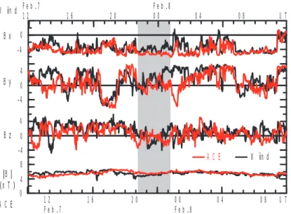
the Earth in the –Y direction and its X position was nearly zero. Figure 1 shows 20 days of hourly magnetic field in GSM and solar wind plasma data from ACE (red) and Wind (black), with 7 February shaded (no convection time delay is considered here). In general, both spacecraft observed the same large-scale heliospheric structure of high-speed solar wind streams, which commonly occur during the declining phase of the solar cycle. The data indicate that the event of interest occurred within a high-speed solar wind stream. The solar wind speed had increased to more than 600 km/s on 6 February. During the time interval of interest from 21:00–24:00 UT on 7 February, the solar wind speed was
∼560 km/s. The solar wind dynamic pressure had a nominal
value of ∼2 nPa.
Close examination of the high-resolution magnetic field data from ACE and Wind reveals that small-scale IMF fea-tures had very poor correlation at the two spacecraft. This is not surprising due to the large separation of the two space-craft, especially in the Y-direction. Figure 2 shows 24 h of higher resolution (92 s) IMF data in GSM from ACE (red) and Wind (black). The time has been shifted by 115 min from ACE to Wind, to match the large-scale structures. This time delay is much larger than the convection time delay from ACE to Wind, ∼44 min, estimated from the solar wind speed and the spacecraft separation along the solar wind flow di-rection. The shaded region corresponds approximately to the time interval of interest in the magnetosphere (21:00– 24:00 UT), as estimated by the solar wind convection time delay from ACE to the magnetosphere, showing very poor correlation between the ACE and Wind IMF observations. At
both spacecraft, the IMF Bzcomponent fluctuated between
north and south directions, but was southward on average for the whole interval of interest. Neither data set appeared to be a good representation of the near-Earth interplanetary conditions for the event, mainly because of the spacecraft’s large distances from the Sun-Earth line. The Polar space-craft entered the magnetosheath briefly during two intervals (22:09–22:10 and 23:18–23:19 UT), but we could not find an appropriate time delay from ACE to Polar so that there would be good correlations between the IMF clock angle and the magnetosheath magnetic field clock angle for both inter-vals. Based on the Polar data, the local magnetic field in the magnetosheath was southward for both intervals of brief magnetosheath excursions.
Figure 3 shows the spacecraft trajectories in the magneto-sphere during the time of interest on 7 February 2002. The
4332 G. Le et al.: Ground-based observations of magnetopause processes � � � � � � �� � � � � � � ��� � � � � � � ��� � � � � � � � ��� � � � � � � � ��� � � � � �� � � � � �� � � � � �� � � � � � � � � � � � � � � � � � � � � � � � � � � � � � � �� � �� � � �� � �� � ��� �� � �� � � � � �� � � �� � � � � � � ����������������������� �� �
� �� � � � ��
Fig. 1. Twenty days of hourly magnetic field and solar wind plasma data from ACE (red) and Wind (black), with the event day 7 February shaded.
left panel of Fig. 3 shows the orbits of Polar (blue), GOES 8 (red) and GOES 10 (green) projected in the GSM XY plane as viewed from the north. The time of interest is a 3-h in-terval from 21:00–24:00 UT on 7 February 2002, although a 13-h orbit segment for Polar is plotted. The Polar spacecraft moves from the Southern to the Northern Hemisphere with the orbit plane nearly in the 14:30 LT meridian plane (marked by the dashed line). The solid black trace is the model mag-netopause from the Petrinec and Russell model (Petrinec and
Russell, 1993) with a subsolar distance of 8.7 RE, which is
scaled by the average positions of the multiple magnetopause crossings observed by the Polar spacecraft (to be discussed in the next section). Thus, the size of the magnetopause ap-peared to be smaller than one would expect based on the nominal solar wind dynamic pressure of ∼2 nPa. In the right panel of Fig. 3, the Polar trajectory and the model magne-topause on the 14:30 LT meridian plane are shown. The solid symbols mark each 30-min interval along the trajectory dur-ing the time of interest, indicatdur-ing that the Polar spacecraft was ideally skimming the vicinity of the magnetopause dur-ing this time interval.
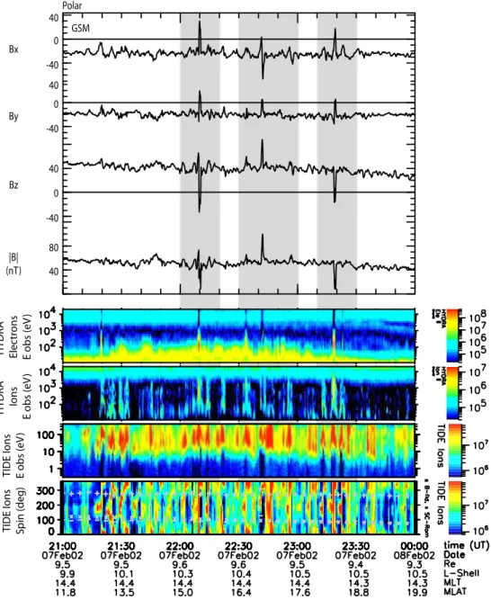
The overview of the 3-h Polar observations is displayed in Fig. 4 showing, from top to bottom, the three components and the magnitude of the magnetic field data in GSM coor-dinates at 6-s time resolution, the HYDRA electron and ion
energy spectrograms, and the TIDE ion energy and spin an-gle spectrograms, respectively. The HYDRA plasma data indicate that the spacecraft stayed inside the magnetopause in the magnetosphere for most of the time, as evident by the presence of hot magnetospheric electrons and ions with en-ergy above ∼2 keV, except for a few short intervals of ∼1– 3 min with marked magnetic deflections that were accompa-nied by the presence of lower energy magnetosheath plasma (a few 10 s eV to ∼1 keV) and the absence of hot magneto-spheric plasma, especially hot electrons. These short inter-vals appeared to be either short excursions into the magne-tosheath (22:09–22:10, 23:18–23:19), partial magnetopause crossings (21:19–21:20, 22:33–22:34) or flux transfer events (22:40–22:43, 22:54–22:57), and will be discussed in detail in the next sections. Starting from ∼21:10 UT, the mag-netic field within the magnetosphere exhibits irregular fluc-tuations of ∼20 nT with period of a few minutes in the Pc5 band. One notable feature in the TIDE data is the presence of cold dense ionospheric ions (∼10–300 eV) occurring as quasi-periodic bursts with periods ∼6 min throughout the interval, similar to the ionospheric ion flow bursts studied by Chen and Moore (2004). The TIDE spin angle spectro-gram indicates that each cold ion burst was associated with
a cycle of inward ( ∼180◦spin angle) then outward (∼0◦or
G. Le et al.: Ground-based observations of magnetopause processes 4333
� �� � � � ��
� � � � � ��� � � � � � � � � � ��� � � � � � � � � � � � � � � � ��� � � � � � ��� � � � � � � �� � � � ���������������� �� � � � �� � �� � � �� � � � � � � � � � � � � � �� � �� � �Fig. 2. High resolution IMF data from ACE (red) and Wind (black). The time has been shifted by 115 min to match the large-scale structures.
15 16 17 18 19 20 21 22 23 0 1 2 3 4 15 17 1819 21 23 0 1 4 X (RE) Y (R E ) 0 2 4 6 8 0 2 4 6 8 ρ (RE) 0 2 4 6 8 Z (R E ) To Sun To D usk
View from the North
0 2 4 6
-2
0230-1430 Local Time Meridian Plane
To N or th 1430 L T 2002 February 7-8 2002 February 7-8 23 22 21 Polar GOES 10 GOES 8 21 22 23 3 Polar MP MP
Figure 3
15 16 17 18 19 20 21 22 23 0 1 2 3 4 15 17 1819 21 23 0 1 4 X (RE) Y (R E ) 0 2 4 6 8 0 2 4 6 8 ρ (RE) 0 2 4 6 8 Z (R E ) To Sun To D uskView from the North
0 2 4 6
-2
0230-1430 Local Time Meridian Plane
To N or th 1430 L T 2002 February 7-8 2002 February 7-8 23 22 21 Polar GOES 10 GOES 8 21 22 23 3 Polar MP MP
Figure 3
Fig. 3. Spacecraft trajectories in the magnetosphere during the time of interest on 7 February 2002. The left panel shows the modelmagnetopause (black) and orbits of Polar (blue), GOES 8 (red) and GOES 10 (green) projected in the GSM XY-plane as viewed from the north. The right panel shows the Polar trajectory and the model magnetopause in the 14:30 LT meridian plane. The solid symbols mark each 30-min interval along the trajectory during time of interest.
Since these dense cold ions are frozen in the closed magnetic flux tubes inside the magnetosphere, their velocity provides a good measure for the motion of the magnetopause bound-ary and the magnetic field lines just inside the magnetopause. The TIDE data show that the magnetic flux tube just inside the magnetopause was oscillating quasi-periodically at pe-riod ∼6 min.
3 Observations of Pc5 magnetic pulsations
In this section, we present coordinated in-situ observations of oscillating magnetopause and magnetospheric magnetic pul-sations at geosynchronous orbit and on the ground that are directly driven.
3.1 Oscillating magnetopause and survace waves
As shown in Fig. 4, several short intervals accompanied no-ticeable magnetic field deflections, both in magnetic field
4334 G. Le et al.: Ground-based observations of magnetopause processes
Figure 4
0 0 0 40 -40 40 -40 40 40 80 -40 Bx By Bz |B| (nT) GSM Polar HYDR A Elec tr ons E obs (eV ) HYDR A Ions E obs (eV )TIDE Ions E obs (eV
)
TIDE Ions Spin (deg)
Fig. 4. A 3-h overview of Polar observations showing, from top to bottom, the three components and the magnitude of the magnetic field data in GSM at 6-s time resolution, the HYDRA electron and ion energy spectrograms, and the TIDE ion energy and spin angle spectrograms, respectively. The signs for flows parallel to the magnetic field direction (+), anti-parallel to the magnetic field direction (−), and opposite
to the spacecraft motion direction (×) are overlaid in the TIDE spin angle spectrogram in the bottom panel. The spin angle of 270◦(90◦)
corresponds to northward (southward) flow direction, and the spin angle of 180◦(0◦or 360◦) corresponds to earthward (sunward) flow
direction.
components and in the field strength. Two of them, at
22:09–22:10 UT and 23:18–23:19 UT, appeared to be netosheath excursions of the Polar spacecraft, as the mag-netic field turned southward and the magmag-netic field strength decreased within the magnetosheath. The details of the mag-netopause crossings are shown in Figures 5a and 5b, respec-tively. Shown in Figs. 5a and b are, from top to bottom, the highest time resolution (8 samples/s) magnetic field data, the HYDRA ion and electron energy spectrograms, the TIDE ion energy and spin angle spectrograms, and the TIDE ion veloc-ity moment data.
The TIDE data are the collapsed 3-D measurements of the cold plasma as 2-D velocity distributions in the spacecraft spin plane, which is nearly aligned with the meridian plane. A detailed description of the TIDE data can be found in Chen
and Moore (2004). The ion velocity components Vxyand Vz,
shown in the bottom panels, are the spin plane velocity pro-jected to the equatorial plane (nearly aligned to the radial direction) and along the Z-axis (north), respectively. They represent roughly the ion velocity perpendicular and paral-lel to the magnetic field, respectively. The positive
G. Le et al.: Ground-based observations of magnetopause processes 4335
Figure 5
HYDR A Ele . E (eV ) Bx GSM B y GSM Bz GSM B (nT ) HYDR A Ion E (eV ) TIDE Ion E (eV ) TIDE Spin (deg) TIDE Vx y (k m/s) TIDE Vz (km/s) -40 0 -40 0 -40 0 40 40 80Magnetosphere Magnetosheath Magnetosphere
40 40 HYDR A Ele . E (eV ) HYDR A Ion E (eV ) TIDE Ion E (eV ) TIDE Spin (deg) TIDE Vxy (km/s) TIDE Vz (km/s) -80 -40 0 40 -80 -40 0 -40 0 40 0 40 80 Bx GSM B y GSM Bz GSM B (nT )
Magnetosphere Magnetosheath Magnetosphere
(a)
(b)
Fig. 5. Magnetopause crossings during the intervals (a) 22:00–22:20 UT and (b) 23:10–23:30 UT. Shown, from top to bottom, are the highest time resolution (8 samples/s) magnetic field data, the HYDRA ion and electron energy spectrograms, the TIDE ion energy and spin
angle spectrograms, and the TIDE ion velocity moment data. The ion velocity components Vxyand Vzshown in the bottom panels are the
spin plane velocity projected to the equatorial plane (nearly aligned to the radial direction) and along the Z-axis (north), respectively.
perpendicular to the magnetic field. The magnetosheath,
marked by the shaded intervals, is characterized by the ab-sence of hot magnetospheric plasma and the preab-sence of magnetosheath plasma. The magnetosheath ions were seen in both the HYDRA and TIDE data, due to their large ther-mal spread from ∼10–1000 eV and the overlap of the instru-ments’ energy ranges.
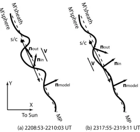
The magnetopause current layer in Figs. 5a and b is char-acterized by sharp southward turnings in the magnetic field at the magnetosphere-magnetosheath transition, occurring at both edges of the shaded intervals. By performing the
minimum variance analysis of the magnetic field data across both the outbound and inbound magnetopause current layer crossings, we find that the magnetopause boundary normal directions exhibited large deviations from the model normal direction in such a way that they were consistent with the passage of a tailward traveling surface wave, as illustrated in
Fig. 6. The vector nmodel is the boundary normal direction
predicted by the Petrinec and Russell magnetopause model, projected in GSM XY plane. The dashed line is
perpendicu-lar to nmodel and represents the local model magnetopause.
4336 G. Le et al.: Ground-based observations of magnetopause processes
Figure 5
HYDR A Ele . E (eV ) Bx GSM B y GSM Bz GSM B (nT ) HYDR A Ion E (eV ) TIDE Ion E (eV ) TIDE Spin (deg) TIDE Vx y (k m/s) TIDE Vz (km/s) -40 0 -40 0 -40 0 40 40 80Magnetosphere Magnetosheath Magnetosphere
40 40 HYDR A Ele . E (eV ) HYDR A Ion E (eV ) TIDE Ion E (eV ) TIDE Spin (deg) TIDE Vx y (k m/s) TIDE Vz (km/s) -80 -40 0 40 -80 -40 0 -40 0 40 0 40 80 Bx GSM B y GSM Bz GSM B (nT )
Magnetosphere Magnetosheath Magnetosphere
(a)
(b)
Fig. 5. Continued.
directions for the outbound and inbound magnetopause cur-rent layer crossings, respectively, obtained from the min-imum variance analysis across the corresponding current layer. In each pair of the magnetopause crossings, the
out-bound crossing occurred first with noutdeflected dawnward
from the model normal direction, and then the inbound
cross-ing with nindeflected duskward. Such a signature is as if an
indention of the magnetopause position caused by a tailward traveling surface wave passes by the Polar spacecraft, as the solid curves schematically illustrate.
We have pointed out the quasi-periodic occurrence of the cold ion bursts observed inside the magnetosphere observed in the TIDE data in Fig. 4. Figures 5a and b also show more details of these cold, dense ion bursts (marked by dashed
lines). These ions are of ionospheric source because of
their narrow thermal spread from ∼10–100 eV, in contrast to those of the magnetosheath proper. They occurred every
∼6 min throughout the interval when the spacecraft was near
the magnetopause in its skimming orbit. During the magne-topause crossings in Figs. 5a and b, the cold ions occurred in the shell immediately earthward of the magnetopause current layer. For the outbound crossings, which indicate that the velocity of the local magnetopause has an earthward com-ponent as the surface wave was passing by, the motion of the cold ions was also moving earthward perpendicular to the magnetic field in the spacecraft orbit plane, as shown
by their spin angle of ∼180◦ and negative velocity
G. Le et al.: Ground-based observations of magnetopause processes 4337
magnetopause was moving sunward, so were the cold ions,
as shown by a spin angle of ∼0◦or 360◦and positive
veloc-ity component Vxy. Thus, it is reasonable to believe that both
the magnetopause and adjacent magnetospheric flux tube os-cillated in phase in response to the surface wave. For all the other ion bursts observed (around the dashed lines) when the spacecraft did not encounter the magnetopause current layer, the ion spin angle showed the similar earthward-then-sunward motion of the flux tubes, presumably in phase with the oscillating magnetopause, and the maximum velocity reached ∼130 km/s. The whole oscillating magnetopause in-terval lasted for ∼3 h at Polar, corresponding to the orbit seg-ment when the spacecraft was skimming the magnetopause at ∼14:30 local time.
3.2 Magnetic pulsations at geosynchronous orbit
The Polar data have shown that the magnetopause and ad-jacent magnetospheric flux tubes were oscillating with an
∼6 min period over an extended time period of ∼3 h,
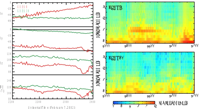
appar-ently in response to the surface wave at the magnetopause. Thus, we examine the GOES magnetic field data in the day-side magnetosphere at geosynchronous orbit to determine the spatial extent of the oscillating magnetospheric field lines. For the time interval of interest, GOES 8 and 10 were in the dayside magnetosphere. Their orbits are shown in Fig. 3 as a red trace for GOES 8 and a green trace for GOES 10. The geosynchronous spacecraft were mainly in the post-noon quadrant. GOES 10 was near local noon moving duskward from ∼11 to 14 local time. GOES 8 was moving duskward from ∼15 to 18 local time.
In the left panel of Fig. 7, the GOES 8 and 10 magnetic field data at 1-min time resolution are shown for the time in-terval of interest. Their dynamic power spectra are shown in the right panels of Fig. 7. Both of the geosynchronous space-craft observed magnetic pulsations in the Pc5 band, which appeared to be correlated to the oscillating magnetopause. First of all, the occurrence of the geosynchronous pulsations was coincident with the occurrence of the magnetic fluctu-ations near the magnetopause observed at Polar. The mag-netic field fluctuations at Polar started at ∼21:10 UT. Ac-cordingly, a noticeable onset of the geosynchronous pulsa-tions occurred immediately after ∼21:10 UT, first at GOES 10 and then at GOES 8 a few minutes later. Secondly, the pe-riods of the geosynchronous pulsations were consistent with the period of oscillating magnetopause of ∼6 min. GOES 10, which was in the subsolar region within 2 h of local noon, ob-served some low-frequency magnetic pulsations with a peak-to-peak amplitude of a few nT. The fluctuations were rather broad-banded in the range of ∼5–10 min with much reduced power. The magnetic pulsations observed by GOES 8, which was a few hours away from local noon, were stronger and much more monochromatic. Their power spectrum was nar-rowly peaked at 2.8 mHz, or 6 min in period, which is sim-ilar to the period of the occurrence of the cold ion bursts and oscillating magnetic flux tubes observed near the mag-netopause by Polar. Thus, strong geosynchronous pulsations
nmodel nin nout V nmodel nin nout V To Sun X Y (a) 2208:53-2210:03 UT (b) 2317:55-2319:11 UT
Figure 6
s/c s/c MP MP M‘ sh e at h M‘ sp he re M‘ sh e at h M‘ sp he reFig. 6. Surface waves at the magnetopause inferred from the
mag-netopause crossings. The dashed line and nmodelare the local
mag-netopause and boundary normal direction predicted by the Petrinec
and Russell magnetopause model. The vectors noutand ninare the
actual boundary normal directions for the outbound and inbound magnetopause current layer crossings, respectively, obtained from the minimum variance analysis. The solid curve illustrates schemat-ically the surface wave at the magnetopause.
occurred only in the limited local time range in the dayside post-noon sector. They were weak near local noon, and they do not appear to continue into the nightside, either. The strongest pulsations at GOES 8 were observed from ∼21:10 to 22:50 UT, or ∼15:55–17:35 LT.
3.3 Magnetic pulsations on the ground
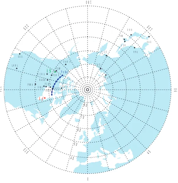
Next we examine coordinated ground-based magnetometer data to determine how the waves at the magnetopause are coupled into the magnetosphere and the ionosphere. Dur-ing the time of the event, the footprints of the Polar space-craft were in the same local time and latitudinal region as the CANOPUS magnetometer array. Meanwhile, the 210-MM array provided simultaneous observations in the morn-ing sector. Figure 8 shows the geographical locations of the ground stations (squares) and spacecraft footprints (dots). In the North American sector, the ground stations include 11 CANOPUS stations at high latitudes and two from the UCLA magnetometer array at mid-latitudes: one at Los Alamos Na-tional Laboratory (LANL) and the other at San Gabriel Dam (SGD) near Los Angeles. The green and red dots are the footprints of GOES 10 and 8 spacecraft, respectively. The connected blue dots are the 4-h ground track of the Polar spacecraft from 20:00 to 24:00 UT, moving westward and marked every 30 min. In the Asian/Pacific sector, 8 ground stations from the 210 MM array are shown.
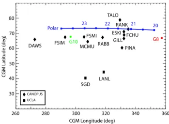
In Fig. 9, the ground stations and spacecraft footprints in the North American sector are shown in the Corrected Geo-Magnetic (CGM) coordinates. The spacecraft footprints are determined by tracing the Tsyganenko 1996 magnetic field
4338 G. Le et al.: Ground-based observations of magnetopause processes � � �� � �� � �� � � �� � �� � �� � � � � � � � � � � � � � � � � � � � � � � � � � � � � � � � � � � � � �� � � � � ��� �� � ��� � � � � � � � �� ��� � � � � � � � � � � �� � �� � � � � � � �� � � � � �� � � � � � Fr equenc y (mHz) Fr equenc y (mHz) 7 5 3 1 2100 2200 2300 2000 2400 7 5 3 1 2100 2200 2300 2000 2400 0 1 2 3 4 5 Log Power (nT 2/Hz) GOES 8 GOES 10
Figure 7
Fig. 7. The GOES 8 and 10 magnetic field data at 1-min time resolution (left panel) and their dynamic power spectra (right panels). The color bar shows the total power of the three components of the magnetic field in logarithm scale.
model under nominal solar wind conditions. For this event, the magnetopause standoff distance is found to be smaller than its nominal value, thus, the actual Polar footprints may be slightly higher in latitude. Since the Polar spacecraft was skimming the magnetopause during the interval of interest, its footprints are expected to be very close to the open-closed field line boundary.
The station TALO was clearly on the open field line that maps to the tail lobe. The station RANK is expected to be near or below the open-closed field boundary. All the other stations are expected to be on closed magnetospheric field lines.
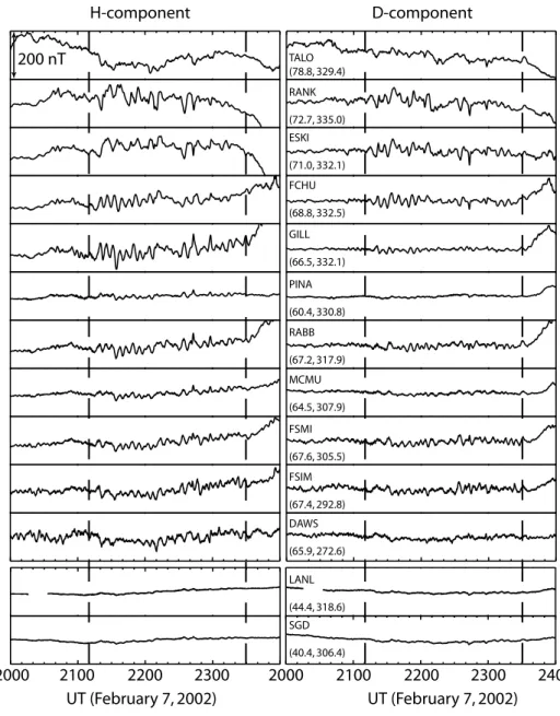
The stacked horizontal components (H and D) of the mag-netic field from the stations in the North American sector are shown in Fig. 10 for a 4-h period from 20:00 to 24:00 UT. In each right panel, the numbers next to the station name give the CGM latitude and longitude of the station. The top 6 panels correspond to those stations along the Churchill meridional line of the CANOPUS array, arranged from high to low latitudes. The next 5 panels are for stations in the east-west line, arranged by their longitudinal distance from the Churchill line. The bottom two panels are for the two mid-latitude UCLA stations. The vertical scale of each panel is 200 nT. The two vertical dashed lines mark the interval between 21:10 UT and 23:30 UT, the time when the oscillat-ing magnetopause and geosynchronous magnetic pulsations were observed. As evident in Fig. 10, geomagnetic pulsa-tions are seen at some CANOPUS stapulsa-tions that appear to be correlated.
Along the Churchill meridional line, strong geomagnetic pulsations with a peak-to-peak amplitude of ∼100 nT can be easily seen in four stations, RANK, ESKI, FCHU and GILL, and their occurrence characteristics are very similar to that of the geosynchronous pulsations at GOES-8, whose
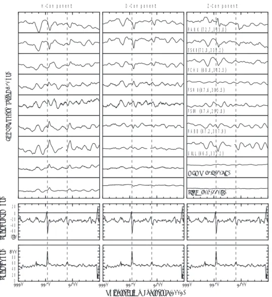
foot-print is ∼25◦ (or ∼01:40 in local time) eastward from the
line. In Fig. 11a, we show the stack plots of power spec-tra for all 6 stations along the meridional line, from high to low latitudes. Note each spectrum has a different base-line as the color-coded dashed base-lines indicate. To compare with the magnetopause oscillation and geosynchronous pul-sations, the power spectra of GOES 8 and GOES 10 magnetic
field data and the Polar TIDE ion velocity moment data (Vxy)
are also shown in Fig. 11.
Multiple spectral peaks are apparent at most stations along
the meridional line. Of special interest is the peak at
2.7 mHz, which appears at all the spectra across the mag-netosphere from the magnetopause, to geosynchrosnous or-bit, to the ground stations. The pulsations at FCHU and GILL are dominated by waves at this frequency. However, the strongest spectral power at this frequency occurred only
at 4 stations, all within ∼6◦ in latitude below the
open-closed field line boundary, namely RANK, ESKI, FCHU and GILL. The power of the spectral peak at 2.7 mHz is one order of magnitude smaller at TALO, the station on open field lines, and about two orders of magnitude smaller at
PINA, the station with the lowest latitude (60.4◦, or 12◦
be-low the open-closed field line boundary). Thus, strong pul-sations only occur at limited latitudes that map to the mag-netopause and outer magnetosphere. This is supported by
G. Le et al.: Ground-based observations of magnetopause processes 4339 � �� �� � �� � � � �� � �� � � �� � � � � � � � � � � � � � � � � � � � � � � �� � � � � � � � �� � � � �� � � � � � � � � � � � � � � � � �� � � � � � � � � � � � � � � �� � � � � � � � � � � �� � � � � � �
� �� � � � ��
G10 G8Fig. 8. Geographical locations of the ground stations (solid squares) and spacecraft footprints (dots). In the North American sector, the ground stations include 11 CANOPUS stations at high latitudes and two from the UCLA magnetometer array at mid-latitudes. The green and red crosses are the footprints of GOES 10 and 8 spacecraft, respectively. The connected blue dots are the 4-h ground track of the Polar spacecraft from 20:00 to 24:00 UT, moving westward and marked every 30 min. In the Asian/Pacific sector, 8 ground stations from the 210 MM array are shown.
the magnetograms of the two mid-latitude stations (two bot-tom panels of Fig. 10), in which we see little evidence of Pc5 pulsations. These observations suggest that the mag-netic pulsations are directly driven by the oscillation of the magnetopause and adjacent flux tubes in the magnetosphere. The stack plots of power spectra for the stations along the east-west line of the CANOPUS array are shown in Fig. 11b, arranged by the longitudinal distance from the Churchill line. The spectrum on the top is for station FCHU, a station in the Churchill line. In comparison, the power of the spectral peak at 2.7 mHz decreases with increasing longitudinal sep-aration from the Churchill line. The three closest stations, RABB, MCMU, and FSMI, all exhibit a similar narrow spec-tral peak at ∼2.7 mHz, and the same onset time and duration for the pulsations, but the spectral power is much reduced at MCMU, presumably due to its larger latitudinal distance
from the open-closed field line boundary (∼8◦). The stations
FSIM and DAWS have the largest longitudinal separation from the Churchill line. They are located westward of the footprint of GOES 10, and so were near local noon during the event. Their spectra seem to be dominated by other unre-lated pulsations, consistent with GOES 10 observations. At DAWS, the dominant pulsation had lower frequency and was present even before the event onset time of ∼21:10 UT.
The coordinated spacecraft and CANOPUS observations presented so far suggest that the correlated pulsations in space and on the ground occur only in a localized region lim-ited both in latitude and local time. The strongest pulsations directly driven by the oscillating magnetopause are limited
within ∼6◦ from the open-closed field line boundary, and
within a longitudinal range from station RABB to the foot-print of GOES 8. For the event interval of 21:10–23:30 UT,
4340 G. Le et al.: Ground-based observations of magnetopause processes
the combined local time range is ∼4 h, from ∼14:00–18:00 local time. To confirm that the pulsations indeed occur in this limited local time region, we examine simultaneous ground-based magnetic field observations from the 210 MM array in the morning sector, as shown in Fig. 12. The CGM latitudes of stations TIX and CHD are similar to that of MCMU and higher than that of PINA, but for the event interval, there is little evidence of coincidental pulsations that are related to those in the post-noon sector. The observations at mid-latitude stations do not show any Pc5 pulsations in the morn-ing sector. Instead, strong Pc3 pulsations are present.
4 Observations of flux transfer events and their foot-prints
4.1 Flux transfer events at the magnetopause
We have shown in Fig. 4 that Polar observed a very strong flux transfer event in the magnetosphere occurring at 22:40– 22:43 UT. This event had the classical FTE signature, which was distinctly different from those of the magnetosheath ex-cursions at 22:09–22:10 UT and 23:18–23:19 UT presented in Sect. 3.1. The strong bi-polar signature was mainly in the X-component in GSM. To display the data in boundary nor-mal coordinates, we found that the model boundary nornor-mal direction did not agree with the instantaneous local boundary normal direction, which is not surprising due to the presence of surface waves on the magnetopause. The local boundary
normal direction at the FTE is found to be deflected ∼37◦,
mainly dawnward, from the model boundary normal direc-tion. Figure 13 shows highest resolution magnetic field data and plasma data from 22:30 to 23:00 UT. The figure is in the same format as Figs. 5a and b except that the magnetic field data here are displayed in the local boundary normal coordinates. The FTE at 22:40–22:43 UT had a very strong bi-polar magnetic field signature of ∼80 nT peak-to-peak in the boundary normal direction. It also had a very strong core field, which at peak is substantially enhanced to about two times the ∼47 nT average magnetospheric field. Thus, the observed FTE has a flux rope structure with a helical mag-netic field inside the core. The observed strong core field combined with the characteristic bi-polar signature strongly argues that it is a reconnection-related phenomenon. It is very unlikely that such a strong core field could be produced by any process other than reconnection, such as magneto-sphere compression due to a pressure enhancement in the so-lar wind.
The HYDRA plasma spectrograms within the core of the FTE show that the magnetospheric hot electrons were almost completely depleted, which is an indication of open flux tube configuration, but the magnetospheric hot ions were only slightly depleted. Meanwhile, the cold ions of ionospheric source are present, but there is very little evidence of the presence of magnetosheath plasma inside the FTE. These ob-servations suggest that the FTE flux rope was just formed a
CANOPUS UCLA 80 70 60 50 40 30
Figure 9
DAWS FSIM G10MCMU FSMI RABB SGD LANL PINA FCHU ESKI GILL G8 Polar TALO RANK 21 20 22 23 CGM Longitude (deg) 260 280 300 320 340 360 CG M La titude (deg)
Fig. 9. The ground stations and spacecraft footprints in the North American sector in the Corrected GeoMagnetic (CGM) coordinates.
short time ago, so that only the hot magnetospheric electrons had time to escape since they are the most mobile species.
The plasma data suggest that this FTE was observed very close to the magnetopause boundary, thus the spacecraft passed through the core of the flux rope. Actually, the space-craft had just made a partial crossing of the magnetopause at 22:33–22:34 UT due to the oscillating magnetopause, as evident by the enhanced flux of the magnetosheath plasma, and earthward-then-sunward motion of the cold ionospheric ions. There was apparently another FTE observed at 22:54– 22:57 UT. This one had a typical bi-polar magnetic signature, but there was no evidence of escaping magnetospheric hot plasma from the flux tube. Thus, it is more likely that Polar did not encounter the core of the FTE flux rope, instead it was in the draping region outside the open flux rope where the magnetic field was compressed but remained closed with both ends connected to the ionosphere. This could happen when the distance between the spacecraft and the instanta-neous magnetopause was greater than the cross-section size of the FTE flux rope in the boundary normal direction,
typi-cally ∼1 RE (Saunders et al., 1984).
4.2 FTE footprints on the ground
Since the first observations of flux transfer events in the spacecraft data (Russell and Elphic, 1978), it has been of great interest to identify their possible ionospheric footprints in ground-based observations. Theories predict that the con-vection of the FTE flux tube generates an Alfv´en wave within the flux tube, which carries a helical magnetic field and a pair of field-aligned currents from the magnetopause to the iono-sphere (Cowley, 1982; Saunders et al., 1984; Southwood, 1987). The closure of the field-aligned currents is through Pedersen currents, and the associated electric field drives a Hall current (Southwood, 1987). The ground magnetic fields produced by the field-aligned currents and Pedersen current cancel each other, and the ground signatures of flux trans-fer events are expected to be transient magnetic perturbations
G. Le et al.: Ground-based observations of magnetopause processes 4341 TALO (78.8, 329.4) RANK (72.7, 335.0) ESKI (71.0, 332.1) FCHU (68.8, 332.5) GILL (66.5, 332.1) PINA (60.4, 330.8) RABB (67.2, 317.9) MCMU (64.5, 307.9) FSMI (67.6, 305.5) FSIM (67.4, 292.8) DAWS (65.9, 272.6) LANL (44.4, 318.6) SGD (40.4, 306.4) H-component D-component 2000 2100 2200 2300 2000 2100 2200 2300 UT (February 7, 2002) UT (February 7, 2002) 2400 200 nT
Figure 10
Fig. 10. The stacked horizontal components (H and D) of the magnetic field from the stations in the North American sector for a 4-h period from 20:00 to 24:00 UT. In each right panel, the numbers next to the station name give the CGM latitude and longitude of the station.
at the footprints associated with Hall current flowing in the ionosphere (Lanzerotti et al., 1986; McHenry and Clauer, 1987; Wei and Lee, 1990; Chaston et al., 1993).
Several theoretical works have been performed to model the ground magnetic signatures associated with traveling field-aligned current systems of FTEs (McHenry and Clauer,
1987; Wei and Lee, 1990; Chaston et al., 1993). In all
these models, the initial FTE open flux tube maps to a cir-cular cross section in the ionosphere as reconnection oc-curs only in a localized patch on the magnetopause. These models consider the motion and evolution of the flux tube footprint and current system in the polar ionosphere and predict that magnetic disturbances are present in all three
components of the geomagnetic field. However, the
de-tails of the predicted magnetic disturbances vary significantly with different models due to the different moving path of
the flux tube and evolving current systems in the model. For example, the magnetic disturbance exhibits a bi-polar signature in the north-south component and a unipolar sig-nature in the east-west and vertical components in McHenry and Clauer (1987). In Chaston et al. (1993), the magnetic disturbances are more complicated varying from bi-polar, unbalanced bi-polar, to unipolar forms in all three compo-nents depending on the ground station’s relative location to the flux tube footprint. In all the models, the predicted mag-netic signatures are traveling disturbances with a speed in the range of 0.5–3 km/s, and thus are best detected using an array of ground magnetic stations. Based on a ∼20-nT detection limit, these models predicted a detection range of ∼600 km in the ionosphere.
The search for FTE signatures in ground magnetic field data has not provided unambiguous results due to the lack
4342 G. Le et al.: Ground-based observations of magnetopause processes FCHU (68.8, 332.5) TALO (78.8, 329.4) RANK (72.7, 335.0) ESKI (71.0, 332.1) GILL (66.5, 332.1) PINA (60.4, 330.8) 2.7 mHz Log Frequency (Hz) 10-4 10-3 10-5 10-2 10-1
(a) CANOPUS Churchill Line
GOES-8 (66.9, 357.3)
Polar TIDE Vxy
GOES-10 (67.7, 296.5) 105 105 105 105 105 105 C ANOPUS Lo g P o w er (nT 2/Hz) 102 103 104 GOES 8 and 1 0 Lo g P o w er (nT 2/Hz) 105 P olar TIDE V elo cit y Lo g P o w er ((k m/s) 2/Hz) 103 102 104 105 2.7 mHz Log Frequency (Hz) 10-4 10-3 10-5 10-2 10-1 FCHU (68.8, 332.5) MCMU (64.5, 307.9) FSMI (67.6, 305.5) FSIM (67.4, 292.8) DAWS (65.9, 272.6) RABB (67.2, 317.9)
(b) CANOPUS East-West Line
GOES-8 (66.9, 357.3) GOES-10 (67.7, 296.5)
Polar TIDE Vxy
Figure 11
Fig. 11. Stack plots of power spectra for the CANOPUS magnetic field, GOES 8 and 10 magnetic field, and the Polar TIDE ion velocitymoment (Vxy). Note the power spectra of the CANOPUS stations have different baselines as indicated by the color-coded dashed lines. (a)
Stations along the Churchill line. (b) Stations along the east-west line. of direct correlation of FTE on the magnetopause and tran-sient signature on the ground (Glassmeier and Stellmacher, 1996). The ground observations were made either at a dif-ferent local time from the in-situ observation (Glassmeier et al., 1984; Elphic et al., 1990), or when there was a lack of in-situ observations (Goertz et al., 1985; Lanzerotti et al., 1986; Sandholt et al., 1992). More recently, a few cases of spacecraft-ground conjunctions were published to report the ionospheric flow response to FTEs (Neudegg et al., 1999, 2001; Wild et al., 2001), which show more conclusively that enhanced ionospheric flow is associated with the FTE at the expected position of the field-aligned current in the FTE.
In this paper, we present direct evidence of transient mag-netic disturbances at the footprint of the FTE flux tube. Two flux transfer events were observed by Polar near the magne-topause at 22:40–22:43 and 22:54–22:57 UT. A close exam-ination of the CANOPUS data in Fig. 10 at the FTE occur-rence times reveals that coincident transient magnetic pertur-bations are indeed evident at all stations except TALO (the station which maps to the tail lobe) and DAWS (the most westward station).
The ground magnetic field signatures associated with the FTEs appear to be a transient unipolar perturbation super-posed on top of the Pc5 pulsations discussed in Sect. 3.3. Fig-ure 14 shows an expanded view of the CANOPUS magnetic
field data as well as the simultaneous Polar Bx-component in
GSM and the field strength. The two dashed lines mark the central cores of the two flux transfer events. The CANOPUS data are arranged by the stations’ magnetic latitudes, from high to low. The FTE ground signatures occurred with a time delay of ∼1 min from the Polar observations. They appeared in the H -component from most stations, except FCHU, as southward unipolar perturbations at stations above FCHU latitude and northward unipolar perturbations below FCHU. The FTE ground signatures in the D-component appeared as a westward perturbation and were strongest in the higher lat-itude stations. In the Z-component, negative perturbations were apparent only in stations along the Churchill line. The amplitudes of the FTE ground perturbations are in the range of ∼15–70 nT, similar to the range predicted by the models
discussed earlier. But the detection range spans over ∼42◦
G. Le et al.: Ground-based observations of magnetopause processes 4343
Figure 12
� �� ��� � �� ��� � � �� � � � ���� � �� ��� � � �� � � �� ��� � �� ��� � � �� � � � � ��� � �� ��� � � �� � � � � ��� � �� ��� � � �� � � � � ��� � �� ��� � � �� � � � � ��� � �� ��� � � �� � � � � ��� � �� ��� � � �� � � �� � � � � � � � � � �� � � � � � � � � � � � � � � � � � � � � � � � � � � � � � � � � � � � � � � � � � � ��� � � � � � � � �� ��� � � � � � � ��� � � � � � � � �� ��� � � � � � � � �� �Fig. 12. The stacked horizontal components (H and D) of the magnetic field from the 210-MM array stations in the Asia/Pacific sector for a 4-h period from 20:00 to 24:00 UT. In each right panel, the numbers next to the station name give the CGM latitude and longitude of the station.
is much larger than the model predictions based on patchy reconnection on the magnetopause.
For the strong FTE observed at 22:40–22:43 UT by the Polar spacecraft, we have used its ground signatures in the
H-component to estimate the propagating time delay from
the spacecraft to CANOPUS ground stations. At Polar, the core of the FTE occurred at 22:41:20 UT, when the Polar
spacecraft mapped to 73.3◦CGM latitude and 310.6◦CGM
longitude at its footprint. The arrival time at the ground sta-tions is taken as the time of the most northward or southward perturbation in the H -component. A timing uncertainty of 5 s is possible since for the time resolution of the CANOPUS data we used 5 s.
We find that the arrival time at the ground station is or-dered by the station’s longitude. Figure 15 shows the time delays from Polar to CANOPUS stations as a function of the longitudinal distance from the Polar footprint. The time de-lay increases as the station’s longitude increases. Thus, the signal moves eastward, or duskward in local time. The solid line is the linear regression of the data, from which we esti-mate that the time delay from the Polar spacecraft to its foot-print is ∼80 s, and the eastward motion of the FTE ground
signature is ∼0.75◦/s. Using the dipolar field line length
from the Polar spacecraft to its footprint, we estimate that the
Alfv´en velocity at which the FTE signature propagates from Polar to its footprint was ∼560 km/s. Previous studies have given a much higher estimate of the Alfv´en velocity in the range of ∼1000 to 2000 km/s near the magnetopause based on the measurement of the magnetic field and thermal plasma (e.g. Burton et al., 1970). However, in this study, the Alfv´en velocity has been significantly reduced, consistent with the presence of cold, dense ion bursts of ionospheric origin near the magnetopause.
4.3 Longitudinal extent of FTE X-line
The longitudinal time delay of the FTE ground signature
shows a ∼0.75◦/s eastward motion, which corresponds to a
speed of ∼31 km/s in the ionosphere. Such a speed is much bigger than the ∼0.5–3 km/s traveling speed one would ex-pect in the ionosphere due to the anti-sunward convection of a FTE flux tube based on the patchy reconnection model of FTEs (McHenry and Clauer, 1987; Chaston et al., 1993). The large speed implies that the reconnection may occur simul-taneously over an extended X-line on the magnetopause and map to an extended longitudinal range in the ionosphere. In this case, at least two factors contribute to the observed large eastward (or duskward) motion of FTE ground signatures in the post-noon dayside sector. First, the ground signature of
4344 G. Le et al.: Ground-based observations of magnetopause processes Figure 13 HYDR A Ele . E (eV ) HYDR A Ion E (eV ) TIDE Ion E (eV ) TIDE Spin (deg) TIDE Vxy (km/s) 0 40 80 -40 0 -40 0 40 80 FTE FTE Partial Crossing BL BM BN B (nT ) 40 TIDE Vz (km/s)
Fig. 13. High-resolution magnetic field data and plasma data from 22:30 to 23:00 UT showing two flux transfer events. The format is the same as Figs. 5a and b, except that the magnetic field data here are displayed in the local boundary normal coordinates.
a duskward propagating perturbation at the equatorial mag-netopause will show similar duskward motion. Second, the length of the magnetic field line from the equatorial magne-topause to its footprint increases from noon to dusk. It takes longer time for a wave at a later local time to propagate along the field line from the equatorial region to the ionospheric footprint, assuming the Alfv´en velocity is the same. This ef-fect alone may result in an eastward time delay on the ground for a signature that simultaneously occurs over a large longi-tudinal range at the equatorial magnetopause.
Assessing the relative contribution of the above two fac-tors has important implications for the nature of FTEs, in particular the longitudinal extent of the reconnection X-line. Using the model magnetopause position scaled by the Polar
observations (shown in Fig. 3), the length of the magnetic field line from the equatorial magnetopause to its ionospheric
footprint is estimated to be ∼11.7 REat the Polar local time
based on a simple dipolar field model. The field line length
is ∼0.6 RE shorter at FSIM local time, and ∼1.3 RE longer
at Churchill line local time. Using the Alfv´en velocity of
∼560 km/s estimated earlier, the varying length of the
mag-netic field line will introduce a time delay of ∼7 s from FSIM to the Polar footprint, and ∼15 s from the Polar foot-print to the Churchill line, or a total of ∼22 s from FSIM to the Churchill line. Since the total observed time delay from FSIM to the Churchill line was ∼53 s (Fig. 15), only an
∼31-s time delay was due to the eastward (duskward)
G. Le et al.: Ground-based observations of magnetopause processes 4345 Figure 14 2240 2300 2220 � � � �� � �� � �� � � � � � � � � � � 100 � �� � � � � � � � � � �� � � � � � � � � � �� � � � � � � � � � � � � ��� � �� ��� � � �� � � � � ���� � �� ��� � � �� � � � � � ��� � �� ��� � � �� � � � � ���� � �� ��� � � �� � � � �� ��� � �� ��� � � �� � � � � � ��� � �� ��� � � �� � � �� � ��� � �� ��� � � �� � C ANOPUS D ata (Sc ale = 140 nT ) -80 2240 2300 2220 2220 2240 2300 PINA (60.4, 330.8) MCMU (64.5, 307.9)
Universal Time (February 7, 2002)
Polar |B| (nT
)
Polar Bx GSM (nT
)
Fig. 14. Expanded view of the CANOPUS magnetic field data, as well as the simultaneous Polar Bx-component in GSM coordinates and the field strength showing the ground signature of flux transfer events.
Figure 16 illustrates how we estimate the longitudinal ex-tent of the reconnection X-line where the flux transfer event occurred, using a simplified dipolar magnetic field model. At the time of the flux transfer event at 22:41:20 UT, mag-netic field lines from the equatorial magnetopause to the ionospheric footprints are drawn at three local times cor-responding to FSIM, the Polar footprint, and the Churchill
line. The longitudinal distance at the equatorial
magne-topause from FSIM to the Churchill line is estimated to be
∼6.6 RE. The flow velocity in the magnetosheath at these
local times ranges from ∼0.2 to 0.5 times the solar wind speed (Spreiter et al., 1966; Spreiter and Stahara, 1980), and we use 0.5 times the solar wind speed, or ∼280 km/s as an upper limit. Now, assume that the reconnection occurred simultaneously along the X-line with a longitudinal extent of X. Since the time delay at the magnetopause from the FSIM local time to the Churchill line local time is ∼31 s,
we have (6.6RE−X)/280 km/s=31 s, which results in a lower
limit of ∼5.2 RElongitudinal extent for the FTE X-line. The
Longitude from Polar Footprint (deg)
T ime D ela y (sec) 60 80 100 120 0 10 20 30 -10 -20 FSIM FSMI MCMU RABB GILL ESKI PINA RANK
Time Delay from Polar FTE at 2241:20 UT
Figure 15
Fig. 15. Time delays of the FTE signature from Polar to the CANO-PUS stations as a function of the longitudinal distance from the Po-lar footprint.
4346 G. Le et al.: Ground-based observations of magnetopause processes � ����� � ��� �� � � � � � � � � � � � � � �� � � �� �� � �� � ��� � � �� � � ���� ���� � � � �� � � � � �� � �� � � � �� ��� �
Figure 16
Fig. 16. Schematic showing the longitudinal extent of thereconnec-tion X-line where the flux transfer event occurred. At the time of the flux transfer event at 22:41:20 UT, magnetic field lines from the equatorial magnetopause to the ionospheric footprints are drawn at three local times corresponding to FSIM, Polar footprint, and the Churchill line, using a simple dipolar magnetic field line. The lon-gitudinal distance at the equatorial magnetopause from FSIM to the
Churchill line is estimated to be ∼6.6 RE.
estimated longitudinal extent is much larger than the scale
size of the flux tube in the boundary normal direction, ∼1 RE
(Saunders et al., 1984).
5 Discussion
Coordinated spacecraft and ground-based observations re-veal that magnetospheric Pc5 pulsations at geosynchronous orbit and on the ground on 7 February 2002, were directly driven by surface waves on the magnetopause boundary at the same frequency. They are the results of forced oscil-lations of the magnetospheric flux tubes in the shell ad-jacent to the magnetopause. Although the Polar observa-tions of the magnetopause and vicinity were made at one local time when it was skimming the magnetopause merid-ian plane at ∼14:30 LT, the simultaneous observations at geosynchronous orbit and on the ground show that the pulsa-tions were not a global phenomenon. Instead, they occurred in a limited local time range of ∼4 h in the post-noon dayside sector (∼14:00–18:00 LT). They did not appear to continue into the nightside sector, near noon, or in the morning sec-tor. The pulsations also occurred only in a limited latitude
range, within ∼6◦of the open-closed field line boundary on
the ground, which maps to a shell extending from the
mag-netopause (with ∼8.6 REstandoff distance) to ∼1 REinward
from the geosynchronous orbit. These observations suggest that the magnetopause oscillations did not occur everywhere
on the magnetopause, and the source mechanism responsible for the observed magnetopause oscillations and surface wave only acted in a limited local time range on the boundary.
Among the possible mechanisms, Kelvin-Helmholz insta-bility, excited when the magnetosheath flow velocity exceeds a certain threshold, is the most cited one for the genera-tion of surface waves at the magnetopause, especially for waves observed near the flanks (e.g. Chen and Kivelson, 1993; Sarafopoulos et al., 2001; Mann et al., 2002). How-ever, in our study, we do not consider the Kelvin-Helmholz instability to be the cause of the observed surface waves and magnetopause oscillations since their occurrence character-istics did not suggest so. Although the event occurred dur-ing a high-speed solar wind stream which favors the K-H instability, the Pc5 waves did not appear to be a global phe-nomenon as shown in other studies (Sarafoupoulos et al., 2001; Mann et al., 2002). They were absent in the dusk flank (past ∼18:00 LT) and in the morning flank, the region where the K-H instability is most effective. Instead, the Pc5 waves excited in the magnetosphere appeared to be a longitudinally localized dayside phenomenon. They were only seen in a limited dayside region within ∼14:00–18:00 local time.
The other possible mechanism for the surface wave and boundary oscillation is fluctuations of the solar wind dy-namic pressure in the same frequency range. During high-speed solar streams, large-amplitude fluctuations in the broad-band Pc5 range are very common in the solar wind (Burlaga and Ogilvie, 1970; Belcher and Davis, 1971). The Pc5 power in high-speed solar wind streams is found to correlate well with the total Pc5 power of the ground-based magnetic field (Kessel et al., 2004). The role of the solar wind dynamic fluctuations is twofold: it could directly drive the magnetopause boundary motion (Wright and Richard, 1995; Kepko et al., 2002) or it could serve as seed perturba-tions of boundary motion to be enhanced by the K-H insta-bility on the flanks (Engbretson et al., 1998). However, given the large-scale size of the high-speed solar wind streams in comparison with the size of the magnetosphere, the magne-tospheric response to the solar wind dynamic pressure fluctu-ations in the Pc5 band is expected to be global over the entire dayside magnetopause. It is unlikely that the observed mag-netopause oscillation on 7 February 2002, which was limited to the ∼14:00–18:00 LT range, was the boundary displace-ment directly driven by the dynamic pressure fluctuations in the high-speed solar wind stream.
Another source of fluctuations of the solar wind dynamic pressure is the localized pressure enhancement generated in the foreshock upstream from the quasi-parallel shock region (e.g. Sibeck et al., 1989; Sibeck, 1990). During the 3-h in-terval of the event, the IMF cone angle was small since the
IMF Bx was the dominant component with a steady,
nega-tive value at both ACE and Wind, and the IMF By
compo-nent fluctuated around zero with a slightly positive average
value (Fig. 2). For a negative IMF Bx, the foreshock region
is expected to be in the dawn side for a positive IMF Byand
the dusk side for a negative IMF By. Thus, for most of the