The Integrated Catchments model of Phosphorus dynamics (INCA-P), a new approach for multiple source assessment in heterogeneous river systems: model structure and equations

HAL Id: hal-00304711

https://hal.archives-ouvertes.fr/hal-00304711

HAL is a multi-disciplinary open access archive for the deposit and dissemination of sci-entific research documents, whether they are pub-lished or not. The documents may come from teaching and research institutions in France or abroad, or from public or private research centers.

L’archive ouverte pluridisciplinaire HAL, est destinée au dépôt et à la diffusion de documents scientifiques de niveau recherche, publiés ou non, émanant des établissements d’enseignement et de recherche français ou étrangers, des laboratoires publics ou privés.

dynamics (INCA-P), a new approach for multiple source

assessment in heterogeneous river systems: model

structure and equations

A. J. Wade, P. G. Whitehead, D. Butterfield

To cite this version:

A. J. Wade, P. G. Whitehead, D. Butterfield. The Integrated Catchments model of Phosphorus dynamics (INCA-P), a new approach for multiple source assessment in heterogeneous river systems: model structure and equations. Hydrology and Earth System Sciences Discussions, European Geo-sciences Union, 2002, 6 (3), pp.583-606. �hal-00304711�

The Integrated Catchments model of Phosphorus dynamics

(INCA-P), a new approach for multiple source assessment in

heterogeneous river systems: model structure and equations

A.J. Wade, P.G. Whitehead and D. Butterfield

Aquatic Environments Research Centre, Department of Geography, University of Reading, Reading, RG6 6AB, UK

Email for corresponding author: andrew.wade4@btinternet.com

Abstract

A new model has been developed for assessing the effects of multiple sources of phosphorus on the water quality and aquatic ecology in heterogeneous river systems. The Integrated Catchments model for Phosphorus (INCA-P) is a process-based, mass balance model that simulates the phosphorus dynamics in both the plant/soil system and the stream. The model simulates the spatial variations in phosphorus export from different land use types within a river system using a semi-distributed representation, thereby accounting for the impacts of different land management practices, such as organic and inorganic fertiliser and wastewater applications. The land phase of INCA-P includes a simplified representation of direct runoff, soilwater and groundwater flows, and the soil processes that involve phosphorus. In addition, the model includes a multi-reach in-stream component that routes water down the main river channel. It simulates Organic and Inorganic Phosphorus concentrations in the land phase, and Total Phosphorus (dissolved plus particulate phosphorus) concentrations in the in-stream phase. In-stream Soluble Reactive Phosphorus concentrations are determined from the Total Phosphorus concentrations and the macrophyte, epiphyte and algal biomasses are simulated also. This paper describes the model structure and equations, the limitations and the potential utility of the approach.

Keywords: modelling, water quality, phosphorus, soluble reactive phosphorus, basin management

Introduction

Most freshwater systems are phosphorus (P) limited and hence there are concerns that increased P loads to a water body can affect the composition and diversity of aquatic plant species and attached algae and phytoplankton by changing the competitive balance, both between the plants, algae and phytoplankton and between the different species of each (Mainstone et al., 2000). In addition, nitrogen (N), generally in the form of nitrate (NO₃), is of concern because it also contributes to nutrient enrichment and elevated concentrations render water unsuitable for drinking. Soluble Reactive Phosphorus (SRP) is derived from both point and diffuse sources, the relative contributions of which are highly variable in space and time. In contrast, NO₃ is derived predominantly from diffuse (agricultural) sources (Jarvie

et al., 2002).

Water quality lies at the centre of European Union (EU) environment policy and is intimately linked to the

hydrogeological and hydro-ecological functioning of river systems. As part of EU legislation that includes the Water Framework Directive, it is necessary to regulate the N and P loads entering lake and river systems considered sensitive to nutrient inputs. The purpose of such regulation is to help mitigate and prevent the problems associated with nutrient enriched water bodies, such as eutrophication and to reduce the water treatment costs for producing water suitable for industrial and public consumption (EC, 2000). Moreover, control measures to regulate the N and P sources are required at the local, regional and national scale to address spatial variations in water quality, whilst maintaining a viable local and national economy.

In the UK, such control measures are of major importance for lowland catchments, particularly in the south and east of England, where the land use is dominated by intensive agriculture and the growing population results in a greater input of nutrients into river systems from Sewage Treatment

Works (STWs). In this region, high evaporation rates coupled with low rainfall reduce the dilution capacity of the rivers, further compounding the enrichment problem (Marsh and Sanderson, 1997). Given the costs involved in reducing N and P loads, mathematical models are used to aid the understanding of freshwater N and P dynamics and to make predictions of future changes in the water quality and ecology under likely scenarios. However, though models of P dynamics have been created, these have tended to address the eutrophication problem in lakes or reservoir systems (Vollenweider, 1975; Kao et al., 1998), or simulate P transport and retention in small-scale, agricultural systems (Gburek and Sharpley, 1998). Moreover, of the models that do simulate P dynamics in both the land and stream components of a catchment, none simulates the impact of P on the aquatic ecology.

This paper describes a new model of P dynamics in river systems named The Integrated Catchments model for Phosphorus (INCA-P), designed to investigate the transport and retention of P in the terrestrial and aquatic environment, and the impacts of the P load on the in-stream macrophyte and algal biomass. This new model builds on the established Integrated Nitrogen in Catchments model, INCA which is a dynamic, process-based hydrochemical model that simulates N in river systems and plot studies, and the ‘Kennet’ model which simulates in-stream P and macrophyte/epiphyte dynamics (Whitehead et al., 1998a, b; Wade et al., 2002a). As such, INCA-P represents an advance towards a generalised framework for simulating water quality determinands in heterogeneous river systems, which started with nitrogen and the INCA model and which could be extended to other determinands.

The INCA-P model

MODEL OVERVIEW

INCA-P is a dynamic, mass-balance model which tracks the temporal variations in the hydrological flowpaths and P transformations and stores, in both the land and in-stream components of the river catchment. INCA-P provides the following outputs:

z daily and annual land-use specific organic and

inorganic-P fluxes (kg P ha–1 _yr–1_{) for all transformation} processes and stores within the land phase;

z daily time series of land-use specific flows (m3 _s–1_{), and} organic and inorganic-P concentrations (mg P l–1_{) in} the soil and groundwaters and in direct runoff;

z daily time series of flows, Total Phosphorus (TP),

Soluble Reactive Phosphorus (SRP) (mg P l–1_{) and}

chlorophyll-a concentrations (µg Chl ‘a’ l-1_{) and}

macrophyte biomass (g C m-2_{) at selected sites along a} river;

z profiles of flow and P concentrations along a river at

selected sites;

z cumulative frequency distributions of flow and P

concentrations at selected sites;

z detailed mass-balance checks.

Spatial data describing the major land use types are required in addition to time series inputs (Table 1). The required time series inputs are:

z the hydrology, namely the Soil Moisture Deficit (mm),

Hydrologically Effective Rainfall (mm day–1_{), Air}

Temperature (o_{C) and Actual Precipitation (mm day}–1_). These data are usually obtained from the MORECS model (Hough et al., 1997);

z data describing land management practices, namely

estimates of growing season for different crop and vegetation types, and fertiliser application quantities and timings which are derived from the Fertiliser Manufacturers’ Association (1994) and local knowledge, respectively;

z the flow rates and SRP concentrations of sewage

effluent inputs.

The model has an interface designed to permit the inclusion of detailed time series data describing growing seasons, fertiliser and STW effluent inputs if available, or alternatively to accept single lumped values thereby allowing the application of the model to systems that are data rich or poor, respectively. To describe the spatial variations in the rainfall, soil moisture deficit and air temperature within a catchment, multiple hydrological time series can be loaded if available.

There are four components to the INCA-P model:

z a GIS interface that defines the subcatchment

boundaries and calculates the area of each land-use type within each sub-catchment;

z a land-phase hydrological model that calculates the flow of effective rainfall through soil water and groundwater stores and as direct runoff. This component drives the water and P fluxes through the catchment;

z the land-phase P model that simulates P transformations and stores in the soil and groundwater of the catchment;

z the in-stream P model that simulates the dilution and

in-stream P transformations, and the corresponding algal, epiphyte and macrophyte growth response.

Table 1. The input data requirements of INCA-P, and examples of typical data sources. *The Centre for Ecology and

Hydrology subsumed the Institute of Terrestrial Ecology in 2000.

Data Description Example Source Reference

TP and SRP streamwater Spot samples taken at points Environment Agency Jarvie et al., 2002

concentrations. within river system. routine monitoring

research studies

Land use Classification at resolution Institute of Terrestrial Ecology* Barr et al., 1993

of 1 km2 _{grid. Land Survey of Great Britain}

Precipitation Daily time series Environment Agency,

Meteorological Office.

Discharge Daily time series Environment Agency

Flow velocity Occasional measurements Environment Agency

for flow ratings

MORECS rainfall, Daily time series (derived) Meteorological Office. Hough et al., 1997

temperature and soil moisture

Base flow index Derived for each flow gauge Centre for Ecology and Gustard et al., 1987

and extrapolated to other Hydrology

tributaries

Fertiliser Practice: Survey Fertiliser Manufacturers’ Fertiliser Manufacturers’

Application Association Association, 1994

Fertiliser Practice: Timing Survey Local knowledge

Growing season Survey Local knowledge

The land-phase component model was developed to

simulate a generic 1 km2 _{cell (Fig. 1). However, since}

INCA-P is semi-distributed rather than fully-distributed, the catchment is not decomposed into an array of cells on a grid basis: the flow of water and P is not routed between cells as with fully-distributed models such as the Système Hydrologique Européen (Abbot et al., 1986). Instead, the catchment is decomposed into three spatial levels (Fig. 2). At level 1, which equates to the largest spatial scale of the three, the catchment is decomposed into sub-catchments. At level 2, each sub-catchment is further decomposed into a maximum of six land use classes; this idea equates to that of a Functional Unit Network (FUN) (Neal, 1997; Wade et

al., 2001). At the third level, the generic cell is then applied

to each land-use type within each sub-catchment. Generalised equations define the P trans-formations and stores within the cell, and six user-defined parameter sets derived through calibration are used to simulate the differences between the land-use types, with one parameter

set mapping to one land-use type. Thus, by calibrating equation parameters using experimental or field data available in the literature, the P fluxes from each transformation is determined. The numerical method for solving the equations is based on the fourth-order Runge-Kutta technique, which allows a simultaneous solution of the model equations thereby ensuring that no single process represented by the equations takes precedence over another. To estimate the water and P outputs from each land-use type within each sub-catchment, the volume and load output from the cell model is multiplied by the land-use area, and the outputs from each land use are summed to provide a total sub-catchment volume and load. The resultant volume and load are then fed sequentially into a multi-reach river model.

The fertiliser, wastewater, slurry and livestock P inputs to the cell model vary with land-use type to simulate the variations in land management practice. In addition, the effective rainfall, soil moisture and temperature can also

Fig. 1. Phosphorus inputs, processes and outputs in the direct runoff, soil and groundwater stores in the cell model of the

land-phase component. TP = Total Phosphorus.

vary between sub-catchments. Thus, it is possible to simulate the spatial variations in land management practice and hydrological inputs to some degree although it is a necessary assumption of this model structure that:

z the fertiliser, wastewater, slurry and livestock inputs are the same for a particular land-use type, irrespective of the location within the catchment;

z the P process rates are the same irrespective of the

location within the catchment, although they can still vary according to spatial variations in the soil moisture and temperature;

z the initial stores of water and P associated with each

land-use type are the same irrespective of the location within the catchment.

This simplified representation of the P dynamics expected in a real river system was chosen to reduce the model’s complexity, the data requirements and the time taken for each model run. Given the complex and highly

heterogeneous nature of flow pathways, P processes and stores, it is uncertain if building a more realistic representation would improve model performance. Moreover, the hydrological and N process simulations produced by the INCA model, which uses the same assumptions and structure appear adequate (Whitehead et

al., 1998b; Wade et al., 2002b). Each of the four components

of INCA-P is described in detail below. THE GIS INTERFACE FOR LAND USE AND SUBCATCHMENT BOUNDARIES

To apply INCA-P to a river system, the main channel is divided into reaches, typically based on the locations of flow or water chemistry sampling locations, or other points of interest. In the case of UK applications, the land area draining into each reach is then derived using the Institute of Hydrology’s Digital Terrain Model and Geographical Information System (GIS) algorithms (Morris and Flavin, 1994). The sub-catchment boundaries are then overlaid onto

Fig. 2. The land-phase component model structure. At level 1 the catchment is decomposed into sub-catchments. At

level 2, the sub-catchments are sub-divided into a maximum of 6 different land-use types. At level three, the soil P transformations and stores are simulated using the cell model. The inset diagram also shows the link between the land-phase and in-stream components at level 1: the diffuse inputs to the stream from the land-phase are added to

STW point source input in each reach and routed downstream.

the Institute of Terrestrial Ecology’s (ITE) Land Cover Map of Great Britain, which is simplified into the six land-use categories: forest, short vegetation (ungrazed), short vegetation (grazed, but not fertilised), short vegetation (fertilised), arable and urban (Whitehead et al., 1998a). These classes were adequate in capturing the spatial variations when modelling nitrogen when using INCA, and therefore are used again in the initial development of INCA-P (Wade et al., 2002b). Moreover, the definitions of the six land use classes are not rigid, and may be changed for the INCA-P applications.

THE LAND-PHASE HYDROLOGICAL MODEL

The MORECS soil moisture and evaporation accounting model is used to convert the actual precipitation time series into an ‘effective’ rainfall time series (HER) (Hough et al., 1997). The effective rainfall is the water that penetrates the soil surface allowing for interception and evaporation loses. The advantage of the MORECS model is that a daily time series of soil moisture deficit is also derived at the same time as the HER, providing essential information for modelling the soil moisture dependent P transformations. The generic cell is split into three units that are defined

according to the major vertical and lateral hydrological pathways likely within a catchment: direct runoff, sub-surface drainage through the soils and groundwater drainage. The ‘direct runoff’ pathway accounts for overland flow, drain and ditch flows and flow over impermeable surfaces, thereby providing a mechanism for the rapid transfer of phosphorus into the main river channel. Direct runoff, in INCA-P, equates to the idea of saturation overland flow, and is assumed to occur when the flow from the soil store exceeds a user defined threshold, ∆. The soil reactive zone is assumed to leach water to the deeper groundwater zone and the river. The split between the volume of water stored in the soil and the groundwater is calculated using the Base Flow Index (Gustard et al., 1987; Wade et al., 2002b).

In INCA-P, the soil drainage volume represents the water stored in the soil that responds rapidly to water inflow. As such, it may be thought of as macropore or piston flow: the flow that most strongly influences a rising hydrograph limb. The soil retention volume represents the water stored in the soil that responds more slowly and may make up the majority of water storage in the soil. As such, this water may be thought of as stored in the soil micropores, and therefore dependent on the soil wetting and drying characteristics. The groundwater volume represents a deeper store in an aquifer, and the residence time may reflect a piston flow effect rather than a more typical groundwater turnover time. The principal residence times for each of the three stores are determined through model calibration.

The flow model is described by Eqns. (1) to (3), the equations that track the mass-balance are listed in Appendix A and the nomenclature is listed in Tables 2 to 5.

Flow change from direct runoff

1 1 2 1 T x x dt dx _{= α} − ₍₁₎

if x2 ≥∆ then input flow = αx2 or if x2<∆ then input flow = 0.

Flow change from soil

2 2 1 2 T x U dt dx ₌ − ₍₂₎

Flow change from groundwater

3 3 2 3 T x x dt dx − =β (3)

where x₁, x₂ and x₃ are the output flows (m3 _s–1 _km–2_{) from} the direct runoff, soilwater and groundwater stores, respectively and U₁ is the hydrologically effective rainfall (m3 _s–1 _km–2_{) as defined by Whitehead et al., (1998a). T}

1, T2 and T₃ are the time constants associated with the three stores (days), α is the proportion of the output soilwater flow

entering the direct runoff flowpath, β is the Base Flow Index and ∆ is the direct runoff threshold flow (m3 _s–1 _km–2_{). Any} input of direct runoff to the groundwater is assumed to occur via the soil water.

The soil retention volume per km2_{, V}

r (m3 km–2) is linearly

dependent on the Soil Moisture Deficit, U₅ (mm) at time, t such that: 1000 . 5 max , U V V_r = _r − (4) where 6 max , =d×p×10 Vr (5)

The factor of 106 _(m2 _km–2_{) is included to maintain the} dimensions of Eqn. (5) in which the units of V_r,max are (m3 _km–2_{). For a 1 km}2 _{cell, V} r can be expressed as ) 1000 . ( .V AV,max U5 A r = r − (6)

where A.V_r,max is the maximum size of the retention volume (m3_{), A is the cell area (km}2_{), d is the soil depth (m) and p is} the soil porosity (Ø). The soil water drainage volume, x₁₆ (m3 _km–2_{) is defined in Appendix A, Eqn. (A.5).}

THE LAND-PHASE P MODEL

The three hydrological stores that form the land-phase hydrological model also form the basis for simulating phosphorus storage within the catchment: INCA-P tracks the organic and inorganic P, within the direct runoff, soil and groundwater stores. The key processes determining the transformation and retention of P within the land-phase are shown in Fig. 1. INCA-P models plant uptake of organic and inorganic P mineralisation, immobilisation and the transformations between firmly bound and available P within each land-use type within each sub-catchment. The plant uptake process varies both in terms of rate and seasonal pattern of uptake to account for the physiological differences between semi-natural vegetation and more intensively managed forestry and farmland. In addition, the plant uptake, mineralisation and immobilisation are soil moisture and temperature dependent and can be set to vary with land-use type.

The inputs from inorganic P fertiliser, wastewater, slurry and the waste from grazing animals are represented as a daily time series of mass (kg P ha–1 _day–1_{) inputs and are} read from a file, if such data are available. Thus, it is possible to simulate multiple fertiliser applications within each year, and multiple plant-growth periods can also be specified. Alternatively, average input rates can be specified for defined time periods. In the groundwater zone, it is assumed that no biogeochemical reactions occur and that a mass

Table 2. Land-phase equation variables

Symbol Definition Units

dx₁/dt Change in direct runoff m3_s-1_day-1 _km-2

dx₂/dt Change in soil flow m3_s-1_day-1 _km-2

dx₃/dt Change in groundwater flow m3_s-1_day-1 _km-2

dx₄/dt Change in readily-available organic phosphorus mass in soil kg P day-1 _km-2

dx₅/dt Change in readily-available inorganic phosphorus mass in soil kg P day-1 _km-2

dx₆/dt Change in readily-available organic phosphorus mass in groundwater kg P day-1 _km-2

dx₇/dt Change in readily-available inorganic phosphorus mass in groundwater kg P day-1 _km-2

dx₈/dt Change in readily-available organic phosphorus mass in direct runoff kg P day-1 _km-2

dx₉/dt Change in readily-available inorganic phosphorus mass in direct runoff kg P day-1 _km-2

dx₁₀/dt Change in firmly-bound organic phosphorus mass in soil kg P day-1 _km-2

dx₁₁/dt Change in firmly-bound inorganic phosphorus mass in soil kg P day-1 _km-2

dx₁₂/dt Change in total organic phosphorus mass input into system kg P day-1 _km-2

dx₁₃/dt Change in total organic phosphorus mass output from system kg P day-1 _km-2

dx₁₄/dt Change in total inorganic phosphorus mass input into system kg P day-1 _km-2

dx₁₅/dt Change in total inorganic phosphorus mass output from system kg P day-1 _km-2

dx₁₆/dt Soil water volume change m3_day-1 _km-2

dx₁₇/dt Groundwater volume change m3_day-1 _km-2

dx₁₈/dt Direct runoff volume change m3_day-1 _km-2

dx₁₉/dt Total water flow input to the system m3_day-1 _km-2

dx₂₀/dt Total water flow output from the system m3_day-1 _km-2

dx₂₁/dt Change in organic phosphorus plant-uptake kg P day-1 _km-2

dx₂₂/dt Change in immobilisation kg P day-1 _km-2

dx₂₃/dt Change in mineralisation kg P day-1 _km-2

dx₂₄/dt Change in organic phosphorus plant-uptake kg P day-1 _km-2

x₁ Direct runoff m3_s-1_km-2

x₂ Soil outflow m3_s-1_km-2

x₃ Groundwater outflow m3_s-1_km-2

x₄ Readily-available organic phosphorus stored in soil kg P km-2

x₅ Readily-available inorganic phosphorus stored in soil kg P km-2

x₆ Readily-available organic phosphorus stored in groundwater kg P km-2

x₇ Readily-available inorganic phosphorus stored in groundwater kg P km-2

x₈ Readily-available organic phosphorus stored in direct runoff kg P km-2

x₉ Readily-available inorganic phosphorus stored in direct runoff kg P km-2

x₁₀ Firmly-bound organic phosphorus stored in soil kg P km-2

x₁₁ Firmly-bound inorganic phosphorus stored in soil kg P km-2

x₁₂ Accumulated total organic phosphorus input to the system kg P km-2

x₁₃ Accumulated total organic phosphorus output from the system kg P km-2

x₁₄ Accumulated total inorganic phosphorus input to the system kg P km-2

x₁₅ Accumulated total inorganic phosphorus output from system kg P km-2

x₁₆ Soil water volume m3 _km-2

x₁₇ Groundwater volume m3 _km-2

x₁₈ Direct runoff volume m3 _km-2

x₁₉ Accumulated water input to the system since simulation start m3 _km-2

x₂₀ Accumulated water output from the system since simulation start m3 _km-2

x₂₁ Accumulated mass associated with organic phosphorus plant-uptake kg P km-2

x₂₂ Accumulated mass associated with immobilisation kg P km-2

x₂₃ Accumulated mass associated with mineralisation kg P km-2

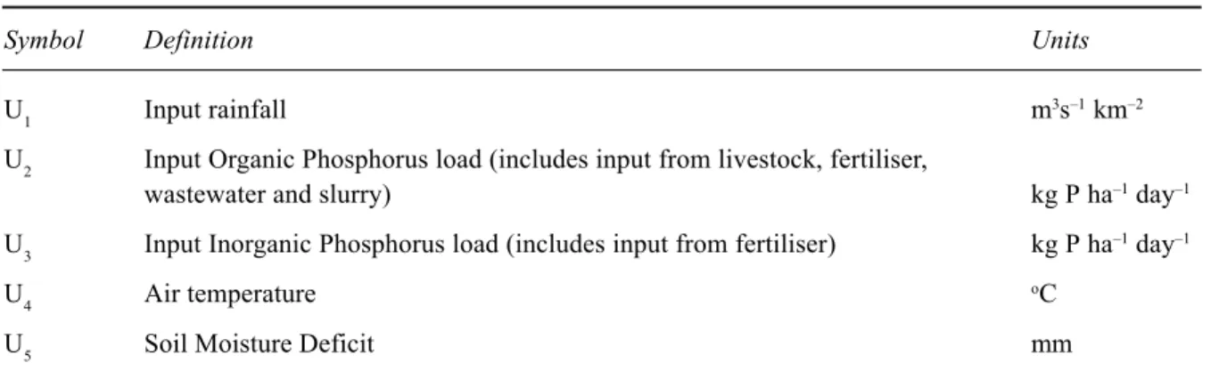
Table 3. Land-phase equations. User supplied inputs as time series.

Symbol Definition Units

U₁ Input rainfall m3_s–1 _km–2

U₂ Input Organic Phosphorus load (includes input from livestock, fertiliser,

wastewater and slurry) kg P ha–1 _day–1

U₃ Input Inorganic Phosphorus load (includes input from fertiliser) kg P ha–1 _day–1

U₄ Air temperature o_C

U₅ Soil Moisture Deficit mm

Table 4. Land-phase equations. User supplied inputs as parameters. *The initial conditions within the model

equations are in terms of kg P km–2_{. However, the user specifies the initial conditions in terms of mg P l}–1_{, and} these concentrations are converted to kg P km–2 _{in the model.}

Symbol Definition Units

α Direct runoff fraction (Ø)

β Base Flow Index (Ø)

∆ Direct runoff threshold m3_s–1 _km–2

T₁ Direct runoff residence time days

T₂ Soil water residence time days

T₃ Groundwater residence time days

C₁ Plant organic phosphorus uptake rate m day–1

C₂ Immobilisation rate m day–1

C₃ Mineralisation rate m day–1

C₄ Conversion rate of readily available organic phosphorus to firmly bound m day–1

C₅ Conversion rate of firmly bound organic phosphorus to readily available m day–1

C₆ Plant inorganic phosphorus uptake rate m day–1

C₇ Conversion rate of readily available inorganic phosphorus to firmly bound m day–1

C₈ Conversion rate of firmly bound inorganic phosphorus to readily available m day–1

C₉ Start of growing season daynumber

C₂₉ Maximum air temperature difference between Summer and Winter o_C

A Area of cell (1 km2_{) km}2

d Depth of soil m

p Soil porosity (Ø)

SMD_max Soil Moisture Deficit maximum value mm

x_4,0 Initial readily available organic phosphorus stored in soil* kg P km–2

x_5,0 Initial readily available inorganic phosphorus stored in soil* kg P km–2

x_6,0 Initial readily available organic phosphorus in groundwater* kg P km–2

x_7,0 Initial readily available inorganic phosphorus in groundwater* kg P km–2

x_8,0 Initial readily available organic phosphorus in direct runoff* kg P km–2

x_9,0 Initial readily available inorganic phosphorus in direct runoff* kg P km–2

x_10,0 Initial firmly bound organic phosphorus stored in soil* kg P km–2

balance of organic and inorganic P is adequate.

The stores of firmly bound P, in organic and inorganic forms are tracked separately from the P assumed to be more easily available for transportation or processing. The inorganic and organic P pools are tracked separately to account for the differences in biochemical cycling, retention and release via the hydrological flowpaths. This conceptualisation also fits in with other, more established models of the plant-soil system P dynamics such as ANIMO (Groenendyk and Kroes, 1999). Whilst it is recognised that P in particulate and soluble forms will move at different rates within the system, it is assumed that the soluble and particulate forms are in equilibrium. Given the uncertainty in the exchange mechanism between the two forms, this assumption was made to simplify the model structure and limit data requirements. The in-stream model requires the P input to be specified as TP and therefore the masses of organic and inorganic P are summed before input to the in-stream component.

Initial conditions are required for the direct runoff, soilwater and groundwater organic and inorganic P concentrations and the user supplies these conditions. To some extent, these initial conditions represent the history of the catchment and the land use at that point in time. The equations for the land-phase component are as follows:

Soil Store

Change in readily available organic P mass in soil

(7)

Change in readily available inorganic P mass in soil

(8)

where x₄ and x₅ are the respective organic and inorganic P

masses (kg P km–2_{) stored in the soil and available to}

microbes, x₁₀ and x₁₁ are the respective firmly-bound organic and inorganic P masses (kg P km–2_{), U}

2 and U3 are the respective organic and inorganic P mass inputs (kg P km–2_). The terms C₁, C₆, C₂, C₃ and are the process rate parameters linked to organic and inorganic P plant uptake, immobilisation and mineralisation, respectively. The terms

S₁ and S₂ are defined in the following paragraphs and the other terms are defined previously.

As for N in INCA, plant P uptake is assumed to be dependent upon the amount of P available, up to a threshold value that represents the maximum uptake needed by the plant. The threshold value can be set by the user and may vary between land-use types.

6 16 2 1 10 x V x S S C Uptake r m n + = (9)

where C_n is the uptake rate (days-1_{) and x}

m is the available

mass of P (kg P). S₁ is a seasonal plant growth index (Ø) (Hall and Harding, 1993), which simulates an increase and decrease in plant nutrient demand based on the time of year:

( )

(

)

where C₉ is the day number associated with the start of the growing season.

Table 5. Model parameters and output concentrations calculated within the land-phase of

the INCA-P model.

Symbol Definition Units

S₁ Seasonal plant growth index (Ø)

S₂ Soil moisture factor (Ø)

S₃ Soil temperature o_C

V_r Soil retention volume m3 _km-2

V_r,max Maximum soil retention volume m3 _km-2

a₁ Soil water organic phosphorus concentration mg P l-1

a₂ Soil water inorganic phosphorus concentration mg P l-1

a₃ Groundwater organic phosphorus concentration mg P l-1

a₄ Groundwater inorganic phosphorus concentration mg P l-1

a₅ Direct Runoff organic phosphorus concentration mg P l-1

a₆ Direct Runoff inorganic phosphorus concentration mg P l-1

dt dx x V x S C x V x S C x V x S S C x V x x U dt dx r r r r 10 6 16 4 2 3 6 16 5 2 2 6 16 4 2 1 1 16 4 2 2 4 10 10 10 86400 . 100 . − + − + + + − + − = dt dx x V x S C x V x S C x V x S S C x V x x U dt dx r r r r 11 6 16 5 2 2 6 16 4 2 3 6 16 5 2 1 6 16 5 2 3 5 10 10 10 86400 . 100 . − + − + + + − + − =

Plant uptake is also assumed to be dependent on the soil moisture where the soil moisture factor, S₂ (Ø) is defined as

max 5 max 2 _SMD U SMD S = − or S₂ = 0 if U₅ > SMD_max (11)

SMD_max (mm) is the maximum soil moisture deficit within a land-use type at which a plant can extract water or at which the soil microbes are active. As such, this point may equate to the wilting point. If the daily soil moisture deficit exceeds the maximum then no P transfers will occur, either because the plants cannot extract water or the microbial activity is suspended. When the soils are wet and equal to or below the threshold, then the process rate is modified by the degree of soil wetness.

Temperature dependency

In addition, it is assumed that all the rate co-efficients are temperature dependent, such that

) 20 ( 3 047 . 1 − = S n C C (12)

where S₃ is the soil temperature (o_{C), calculated from a} seasonal relationship dependent on air temperature, U₄ (o_C) where ) 365 2 3 sin( 29 4 3 dayno C U S = − π (13)

where C₂₉ is the maximum difference (o_{C) between the} summer and winter temperature (Green and Harding, 1979).

Mineralisation and immobilisation

The fluxes of P associated with mineralisation and immobilisation are defined as

6 16 4 2 3 _{V x} 10 x S C ion ineralisat M r + = (14) 6 16 5 2 2 10 x V x S C tion Immobilisa r + = (15)

where all the terms have been defined previously. Both terms are soil moisture and temperature dependent, and a function of P concentration.

Groundwater store

Change in mass of organic phosphorus in groundwater

17 6 3 16 4 2 6 .86400 .86400 x x x x V x x dt dx r − + = β (16)

Change in mass of inorganic phosphorus in groundwater

17 7 3 16 5 2 7 .86400 .86400 x x x x V x x dt dx r − + = β (17)

where x₆ and x₇ are the masses of organic and inorganic P

stored in the groundwater (kg P km–2_{) and x}

17 is the groundwater volume (m3 _km–2_).

Direct runoff

Change in mass of organic phosphorus in direct runoff

18 8 1 16 4 2 8 .86400 .86400 x x x x V x x dt dx r − + =α (18)

Change in mass of inorganic phosphorus in direct runoff

18 9 1 16 5 2 9 .86400 .86400 x x x x V x x dt dx r − + =α (19)

where x₈ and x₉ are the masses of organic and inorganic P associated with the direct runoff (kg P km–2_{) and x}

18 is the direct runoff volume (m3 _km–2_).

Firmly bound phosphorus in soil store

Change in mass of firmly-bound organic phosphorus in soil

16 6 10 5 16 6 4 4 10 10 10 x V x C x V x C dt dx r r + − + = (20)

Change in mass of firmly-bound inorganic phosphorus in soil 16 6 11 8 16 6 5 7 11 10 10 x V x C x V x C dt dx r r + − + = (21)

where x₁₀ and x₁₁ are the masses of organic and inorganic P associated with the firmly bound P stored in the soil (kg P km–2_{). C}

4 and C7 are the transfer rates of organic and in-organic P respectively, from the readily available store to the firmly bound store. C₅ and C₈ are the transfer rates of organic and inorganic P, from the firmly bound store to the readily available store.

Calculation of concentrations

The concentrations of inorganic and organic P in the three hydrological stores are calculated as the load divided by the volume of the store. For example, for organic phosphorus in the soil, a₁ (mg P l–1_): r V x x a + = 16 4 1 1000 . (22)

where x₄ is the mass output per day from the soil store, and (x₁₆ + V_r) is the volume of the soil store. The factor of 1000 arises because of the conversion units required to generate a concentration in mg P l–1_.

THE IN-STREAM P PROCESS MODEL

The in-stream P process model represents the major stores in the aquatic P cycle and the in-stream processes that determine the transfer of P between those stores (Fig. 3). This component is similar to the Kennet Model, though it has been written in terms of mass rather than concentration to overcome the mass-balance problems identified by Wade

et al. (2002b). The in-stream model is a multi-reach, dynamic

representation that operates on a daily time step. It simulates the mean daily flow, the Total Phosphorus (TP), Soluble Reactive Phosphorus (SRP), Boron and suspended sediment

streamwater concentrations in the water column, the SRP concentrations in the pore water and TP associated with the river bed sediments. Boron was modelled because it is a chemically conservative tracer of point source inputs, and therefore valuable for testing in-stream mixing relationships (Neal et al., 2000; Wade et al., 2002c). The equation used to simulate Boron could be applied equally to any other determinand assumed to behave conservatively. For example chloride could be used although a correction may be needed for atmospheric sources. In addition, the model simulates the re-suspension of bed sediment, the deposition of suspended sediment and the effects of the P concentrations on the growth of the macrophyte and epiphyte populations within the reach, and the subsequent feedback that such growth has on the water column TP and SRP concentrations. Inputs to the model are the flows and TP loads derived from the land phase component of INCA-P.

Streamwater TP and SRP concentrations are simulated in this first instance because TP is a measure of the total amount of P in the system, and therefore is useful for mass balance, whilst SRP is a measure of the dissolved P in the streamwater that is biologically available. It is assumed that TP is the sum of SRP+PP+SUP where PP is the particulate phosphorus and SUP is the soluble unreactive phosphorus. Mass-balance equations are used to quantify the amount of P (and carbon in the case of the macrophytes and epiphytes, and chlorophyll ‘a’ in the case of algae) associated with the different stores in the aquatic P cycle (Eqns. 23–48). The rates of mass transfer between the stores are modelled as first-order (linear) exchanges and these rates are represented as parameters in the equations. However, whilst the equations comprise linear exchanges, the combined response of feedbacks and temperature dependencies ensures the response is non-linear. The inputs, outputs, parameters and variables are listed in Tables 6 to 9 and the equations to check the mass-balance are presented in Appendix B. The terms P_in, B_in, S_in, L_in and D_in used in the following equations are defined in Appendix C.

If available, effluent time series describing the effluent flow (m3 _s–1_{), and TP (mg P l}–1_{) and boron (mg B l}–1₎ concentrations are used to describe the inputs from STWs entering each reach in the system. Alternatively, constant values for the effluent flow and TP and B concentrations can be used.

The changes in water storage in the reach are represented using a simple linear-reservoir routing method, modified to account for the lateral and STW flow inputs. The differential equation used to model the flow within the reach is

4 25 7 5 4 25 ( ) T x U S S dt dx ₌ + + − ₍₂₃₎

where x₂₅ = the flow out of the reach at time t (m3_s–1_{), S}

4 =

the upstream flow into the reach at time t (m3_s–1_{), S}

5 = the

lateral inflow into the reach at time, t (m3_s–1_{), U}

7 = the STW

flow into the reach at time t (m3_s–1_{) and T}

4 = the flow storage

time constant (days) defined as

86400 . 25 4 _axb L T = (24)

Thus, the time constant, T₄ is estimated from the reach length, L divided by the flow velocity, v which is itself estimated from the discharge using the expression _{v ax}b

25

= ,

where a and b are constants. The values of a and b can be determined from tracer experiments or from flow-velocity relationships derived at discharge gauging stations (Whitehead et al., 1979).

Given that P is attached to both the suspended and bed sediments, it is necessary to estimate the amount of sorption

and desorption between the P in the water and that associated with the suspended and bed sediments (Fig. 3). To achieve this, an estimate of the mass of bed sediment is calculated from estimates of the reach length and width, and an estimate of the depth of the material that could potentially be re-suspended. This bed mass is modified, at each time step, by an estimate of the amount of material re-suspended or deposited. This amount is determined from the change in grain size with flow: a cumulative frequency curve for bed sediment has been measured in the River Lambourn, S. England and, for a given grain size, the fraction of the bed that is held in suspension is estimated (Evans, 2002). The use of grain size data measured in the Lambourn is a starting strategy and, in the absence of similar data for other rivers, an assumption is made that the bed sediments of the Lambourn and other rivers are similar. This data extrapolation was made to permit the development of INCA-P and further work will be necessary to determine the importance of this assumption when the model is applied to other river systems.

The equation for the change in mean grain diameter of the bed material suspended at time t, x₂₆ (µm) is

    + + − = 4 25 7 5 4 10 26 T x U S S C dt dx (25) where C₁₀ = a constant relating the flow in the reach to the mean grain diameter re-suspended or deposited from the

overlying water column onto the stream bed (µm s m–3_).

Whilst the change in grain diameter that is re-suspended or deposited is a function of the shear velocity and the channel roughness (Chow et al., 1988; Miller et al., 1977), a simple linear relationship between flow and grain diameter was used as a first approximation to limit the model’s complexity. The change in grain size held in suspension was converted into a mass contribution to the suspended sediment mass at time t, x₂₇ (kg) using the following equation

dt dx dx dPM dt dx 26 26 27 ₌ (26)

where PM = the potentially movable bed mass (kg),

x₂₆ = the mean grain diameter of the bed material (µm). The change in the potentially available bed material with grain diameter is estimated as

wLf x CV dx dPM 28 26 . ∆ = (27)

where ∆CV is the slope of the curve relating the cumulative fraction of the bed material to the grain size (µm-1_{), x}

28 is

Table 6. Model parameters and output concentrations calculated within the in-stream phase of the INCA-P model.

Symbol Definition Units

dx₂₅/dt Change in the in-stream flow m3_s-1_day-1

dx₂₆/dt Change in the mean grain diameter kg day-1

dx₂₇/dt Change in the suspended sediment deposited or resuspended kg day-1

dx₂₈/dt Change in reach bed mass kg day-1

dx₂₉/dt Change in suspended sediment stored in the reach kg day-1

dx₃₀/dt Change in Boron stored in reach kg B day-1

dx₃₁/dt Change in macrophyte biomass stored in water column in reach g C day-1 _m-2

dx₃₂/dt Change in epiphyte biomass stored in water column in reach g C day-1 _m-2

dx₃₃/dt Change in Total Phosphorus stored in water column in reach kg P day-1

dx₃₄/dt Change in Total Phosphorus stored in pore water in reach kg P day-1

dx₃₅/dt Change in live algae stored in water column in reach µg Chl ‘a’ day-1

dx₃₆/dt Change in dead algae stored in water column in reach µg Chl ‘a’ day-1

dx₃₇/dt Change reach volume m3 _day-1

dx₃₈/dt Change in flow volume into reach m3 _day-1

dx₃₉/dt Change in flow volume out from reach m3 _day-1

dx₄₀/dt Change in Total Phosphorus input to reach kg P day-1

dx₄₁/dt Change in Total Phosphorus output from reach kg P day-1

dx₄₂/dt Change in epiphyte uptake in reach kg P day-1

dx₄₃/dt Change in Total Phosphorus due to water column/pore water SRP exchange kg P day-1

dx₄₄/dt Change in Total Phosphorus co-precipitated with calcite kg P day-1

dx₄₅/dt Change in Total Phosphorus in water column due to PP re-suspension from bed kg P day-1

dx₄₆/dt Change in Total Phosphorus in water column due to PP deposition on bed kg P day-1

x₂₅ In-stream reach outflow m3_s-1

x₂₆ Mean grain diameter µm

x₂₇ Suspended sediment deposited or resuspended kg

x₂₈ Reach bed mass kg m-2

x₂₉ Suspended sediment stored in the reach kg

x₃₀ Boron stored in reach kg B

x₃₁ Macrophyte biomass stored in water column in reach g C m-2

x₃₂ Epiphyte biomass stored in water column in reach g C m-2

x₃₃ Total Phosphorus stored in water column in reach kg P

x₃₄ Total Phosphorus stored in pore water in reach kg P

x₃₅ Live algae stored in water column in reach µg Chl ‘a’

x₃₆ Dead algae stored in water column in reach µg Chl ‘a’

x₃₇ Reach volume m3

x₃₈ Flow volume into reach m3

x₃₉ Flow volume out from reach m3

x₄₀ Accumulated Total Phosphorus input to reach kg P

x₄₁ Accumulated Total Phosphorus output from reach kg P

x₄₂ Accumulated epiphyte uptake in reach kg P

x₄₃ Accumulated Total Phosphorus due to water column/pore water SRP exchange kg P

x₄₄ Accumulated Total Phosphorus co-precipitated with calcite kg P

x₄₅ Accumulated Total Phosphorus in water column due to PP deposition on bed kg P

Table 7. Input time series, constants and time series calculated within the model.

Input variable Description Units

TIMESERIES

U₇ STW flow into reach at time, t m3 _s-1

U₈ Suspended sediment at time, t mg Sed l-1

U₉ Boron concentration in sewage effluent at time, t mg B l-1

U₁₀ TP concentration in sewage effluent at time, t mg P l-1

U₁₁ Solar Radiation at time, t Normalised 0-1

CONSTANTS

L Reach length m

w Reach width m

a Velocity-discharge parameter m-2

b Velocity-discharge parameter (Ø)

DCV Change in grain size suspended µm-1

f Fraction of the total bed material that is available for resuspension (Ø)

PM Change in potentially moveable bed mass with respect to grain diameter kg

CALCULATED

S₄ Upstream flow into reach at time, t m3 _s-1

S₅ Lateral inflow into reach m3 _s-1

S₆ Upstream Total Phosphorus concentration at time, t mg P l-1

S₇ Upstream Boron concentration in water column at time, t mg B l-1

S₈ Upstream concentration of live algae at time, t µg Chl ‘a’ l-1

S₉ Upstream concentration of dead algae at time, t µg Chl ‘a’ l-1

B_in Total Boron input to reach at time, t kg B day-1

P_in Total Phosphorus input to reach at time, t kg P day-1

S_in Suspended sediment input to reach at time, t kg day-1

L_in Live algae input to reach at time, t µg Chl ‘a’ day-1

D_in Dead algae input to reach at time, t µg Chl ‘a’ day-1

material that is available for re-suspension (Ø) and w is the reach width (m).

The change in moveable bed mass at time t, x₂₈ (kg m-2_{) is} expressed using the following equation

dt dx Lw dt

dx28 ₌ 1 27 (28)

where all the terms have been defined previously. The equation is an expression of the mass of sediment that is gained or lost from the bed following the re-suspension or deposition of sediment.

The in-stream suspended sediment concentration is assumed to depend on the material that enters the reach, plus or minus that material which is resuspended or deposited, respectively. When Eqn. (26) is negative then the grain size held in suspension falls and the term becomes negative, thereby allowing the simulation of deposition in Eqn. (29), which represents the suspended sediment, x₂₉ (kg)

in the reach dt dx x x x S dt dx in 27 37 25 29 29 _{= −} 86400_{+ (29)}

where S_in = the upstream suspended sediment mass at time,

t (kg day-1_{) and x}

37 is the reach volume (m3).

The equation for the change in the mass of Boron, x₃₀ (kg B) in the reach is 37 25 30 30 86400 x x x B dt dx in− = (30)

where B_in = the total mass of B entering the reach at time, t (kg B) and x₃₀ = the B mass in the water column (kg B).

It is assumed that the B within the reach is entirely STW derived and there is no B in the lateral inflow (Neal et al., 2000). Boron is also assumed to be conservative; as such it does not take part in any reactions within the river reach and can be modelled using a simple input-output

mass-Table 8. Model parameters.

Parameter Description Units Value or range Reference

given in or derived from the literature

C₁₀ Sediment resuspension/ settling µm s m–3 _{1–10 Est.}

C₁₁ Macrophyte growth rate day–1 _{0.1–0.8 Dawson, 1976;}

Wright et al.,1982

C₁₂ Self-shading for macrophytes gC m–2 _{74 Dawson, 1976}

C₁₃ Half-saturation of P for macrophyte growth mg P l–1 _{0.0002–0.496 Bowie et al., 1985}

C₁₄ Macrophyte death rate s m–1 _{g C}–1 _day–1 _{0.01–0.3 Chapra, 1997}

C₁₅ Epiphyte growth rate m2 _{g C}–1 _day–1 _{0.004–0.04 Chapra, 1997}

C₁₆ Half-saturation of P for epiphyte growth mg P l–1 _{0.0002–0.496 Bowie et al., 1985}

C₁₇ Epiphyte death rate s m-3 _day–1 _{0.01–0.05 Bowie et al., 1985}

C₁₈ Proportion of P in epiphytes g P g–1 _{C 0.0054 Dawson, 1976}

C₁₉ P exchange (water column\ pore water) m3 _day–1 _{0.4–86.4 Wagner and}

Harvey, 1997

C₂₀ Precipitation of P in water column m3 _day–1 _{0.68 House et al., 1995}

C₂₁ Bed (bulk) sediment depth m 0.1–1.0 Est.

C₂₂ Proportion of P in macrophytes g P g-1 _{C 0.0054 Dawson, 1976}

C₂₃ Algal death rate day–1

C₂₄ Algal growth rate day–1

C₂₅ Half-saturation of P for algal growth mg P l–1

C₂₆ Self-shading for algae µg Chl ‘a’ m-2

C₂₇ Settling rate of dead algae day–1

C₂₈ K_dbed_{for bed sediment (as a fraction of K}

dsus) (∅) 0.1–1.0 Jarvie et al., 2002

K_dsus _K

d for suspended sediment dm3 kg–1 200 Jarvie et al., 2002

θM Macrophyte temperature dependency (∅) 1.01–1.066 Bowie et al., 1985

θE Epiphyte temperature dependency (∅) 1.01–1.066 Bowie et al., 1985

θA Algal temperature dependency (∅) 1.01–1.066 Bowie et al., 1985

n Porosity (∅) 0.3 Chow et al., 1988

ρs Bulk sediment density kg m–3 2.65 Chow et al., 1988

Table 9. Output concentrations calculated within the in-stream phase of the INCA-P model.

Symbol Definition Units

a₇ Water column suspended sediment concentration mg l–1

a₈ Water column total phosphorus concentration mg P l–1

a₉ Water column Boron concentration mg B l–1

a₁₀ Pore water total phosphorus concentration mg P l–1

a₁₁ Water column soluble reactive phosphorus concentration mg P l–1

a₁₂ Pore water soluble reactive phosphorus concentration mg P l–1

a₁₃ Water column live algae concentration µg Chl ‘a’ l–-1

+ + − − = − a C Lw a U x x C C x x x P dt dx U E in 11 16 11 11 31 32 ) 20 ( 15 18 37 25 33 33 1 1000 ). ( 86400 _θ 4 ( )       + − − loss gain a C a a C 11 20 11 12 19 1000 1000 balance equation.

The differential equation used to model the change in the macrophyte biomass, x₃₁ (g C m–2_{) flow within the reach is} (31) where

θM = macrophyte temperature dependency (Ø),

C₁₁ = the macrophyte growth rate (day–1_),

C₁₂ = the constant associated with macrophyte self-shading (g C m–2_),

C₁₃ = the half saturation constant associated with the macrophyte growth (mg P l–1_),

C₁₄ = the macrophyte death rate (s m–1 _{g C}–1 _day–1_),

U₁₁ = solar radiation,

a₁₂ = the pore water SRP concentration (mg P l–1_{) and}

U₄ = water temperature (O_C).

The general form of Eqn. (31), which simulates the interactions between the macrophytes and the epiphytic algae, is based on the Lotka-Volterra model of predator-prey interactions (Lotka, 1926; Volterra, 1926). In this case, the macrophytes are considered as the “prey” and the epiphytic algae as the “predator”. Whilst the coexistence of macrophytes and epiphytes is not a true predator-prey relationship, the Lotka-Volterra model does generate the expected relational changes in biomass. Unmodified formulations of the original Lotka-Volterra predation model produce peak biomass estimates that are mainly dependent on the initial conditions (Hastings, 1997). As such, the basic Lotka-Volterra model has been modified as follows. The first order growth rate, C₁₁ is dependent upon the substrate (pore water) SRP concentration (Thornley, 1976). This dependency is described by the Michaelis-Menten

formulation, in which the half-saturation constant, C₁₃

represents the substrate concentration at which growth is half the maximum. As such, the parameter, C₁₃ dictates at what level the substrate becomes limiting. The term for the macrophyte growth also is modified to account for the seasonal variations in solar radiation and water temperature. The second term, which includes the product of the macrophyte and epiphyte biomass, x₃₂x₃₁, on the right hand side of Eqn. (31) quantifies the effect the impact of the epiphytic algae has on the macrophyte mortality. This term is also flow dependent to account for the wash out of macrophytes from the reach under high flow conditions.

The change in epiphyte biomass stored in reach at time t,

x₃₂ (g C m-2_{) is represented by the following equation} 25 32 17 11 16 11 11 31 32 ) 20 ( 15 32 4 _{C x x} a C a U x x C dt dx U E ₋ + = − θ ₍₃₂₎ where

θE = epiphyte temperature dependency (Ø), C₁₅ = the epiphyte growth rate (m2 _{g C}–1 _day–1_),

C₁₆ = the half saturation constant associated with the epiphyte growth (mg P L–1_),

C₁₇ = the epiphyte death rate (s m-3 _day–1_{) and}

a₁₁ is the water column SRP concentration (mg P l–1_).

The term ( ) 11 16 11 11 20 15 a C a U C T E + −

θ _{from Eqn. (32) quantifies the}

epiphyte growth. As in the case of the macrophytes, it is based on the Michaelis-Menten formulation but with a dependency upon the SRP available in the water column in addition to the water temperature and the solar radiation. The death rate of the epiphytes is also flow dependent. The change in the TP in the water column at time t, x₃₃ (kg P) is represented by the following equations

(33) where dt dx x wLC n gain s 27 34 21 ) 1 ( 1 − = ρ , if dt27>0 dx ₍₃₄₎ and dt dx K a loss SUS D 27 11 6 10− = , if 27 _≤0 dt dx ₍₃₅₎ where

P_in = the total mass of P entering the reach at time,

t (kg P),

C₁₈ = the ratio of phosphorus to carbon in epiphytes (g P g C-1_),

C₁₉ = the constant associated with the exchange of SRP between the pore water and the overlying water column (m3 _day-1_),

C₂₀ = the constant associated with the co-precipitation of P with calcite in the water column (m3 _day-1_),

C₂₁ = the bulk sediment depth (m),

x₃₄ = the TP mass associated with the bed sediment

(kg P),

Sus D

K = K_d for suspended sediment (dm3 _kg-1_),

Bed D

K = K_d for bed sediment (dm3 _kg-1_),

n = the porosity (∅),

r_s = the bed sediment bulk density (kg m-3_).

The K_d values are a measure of the affinity of the solid phase for sorbing P from the surrounding substrate (House et al., 1995; House and Warwick, 1999).

25 31 32 14 31 12 12 13 12 12 11 31 ) 20 ( 11 31 ) )( ( 4 x x x C x C a C a C U x C dt dx U M ₋ + + = θ −

It is assumed that the TP concentration of the water column is determined by the amount of phosphorus entering the reach (from both upstream and the STW), epiphyte uptake, sorption/desorption of P to and from the suspended sediment, exchange of P between the pore water and water column and the precipitation of P (Fig. 3). As such, the estimate of the change in the TP concentration is based only on changes in the PP and SRP: it is assumed that any SUP present, by definition, does not take part in any reactions.

The TP concentration input to the reach is calculated from the mass balance of all the known P sources: upstream, STW and lateral flow inputs. The first and second terms on the right hand side of Eqn. (33) represent the input and output of TP to and from the reach, respectively. The third term represents the uptake of SRP by the epiphytic algae. As such, the term is described in more detail with reference to epiphyte biomass Eqn. (32). The fourth term on the right hand side of Eqn. (33) represents the exchange of SRP between the pore water and the overlying water column. When the pore water concentration is greater than that of the overlying water column then there is a net transfer of SRP to the overlying water column. Conversely, if the SRP concentration is greater in the overlying water column compared to the pore water, then SRP is transferred to the pore water. The fifth term represents the loss of SRP from the water column by co-precipitation with calcite. The final term represents the loss of total phosphorus from the water column to the stream bed by sediment deposition or the gain of PP from the bed during periods of resuspension. Given

dt

dx27 _{can be both positive and negative, then the sign}

represents the addition or subtraction of PP from the TP store in the water column. It is assumed that PP in suspension in the water column is in equilibrium with the surrounding SRP in the water column and that the PP associated with the stream bed is in equilibrium with the surrounding SRP in the pore water. The gain and loss terms reflect these equilibrium conditions, which are expressed in terms of K_d values. It is assumed that Bed

D

K ≤ Sus D

K , since the sediment

in suspension will sorb more SRP than the bed sediment. For the purposes of estimating suitable values for Bed

D

K and

Sus D

K both are assumed to lie in the range 100 to 300 dm3

kg–1_{, which is the range specified for bed sediment by Jarvie}

et al., (2002). As such, Sus D

K is chosen from this range

and Bed D K is estimated as a fraction, C₂₈ (0.1 to 1.0) of Sus D Bed D C K K = ₂₈ (36)

The equation for the change in the TP associated with the river bed, x₃₄ (kg P) in the reach is

(37) where dt dx x wLC n loss s 27 34 21 ) 1 ( 1 − = ρ , if _dt27 >0 dx ₍₃₈₎ and dt dx K a gain SUS D 27 11 6 10− = , if 27 _≤0 dt dx (39) where C₂₂ = the ratio of phosphorus to carbon in macrophytes (g P g C-1_).

It is assumed that the TP associated with the river bed is affected by three factors.

z The mass of phosphorus sorbed on the bed sediment.

As such, the gain and loss term on the right hand side of Eqn. (37) represents the movement of PP between the stream bed and the overlying water column due to deposition (a gain of PP to the stream bed) and re-suspension (a loss of PP from the stream bed).

z The interaction between the SRP associated with the

pore water and the overlying water column. The conversion ratio of P:C relates the mass of P removed from the pore water to the changes in macrophyte biomass, which is measured in terms of carbon (Dawson, 1976).

z The uptake of SRP from the pore water during periods

of macrophyte growth.

The pore water depth, p cannot be greater than the bulk sediment depth. As such, the pore water depth is estimated as a fraction, n of the bulk sediment depth, C₂₁. The fraction equates to the porosity, namely,

21

nC

p = (40)

The equations for the change in live and dead biomass of algae within the reach are those developed by Whitehead and Hornberger (1984). The change in live algae stored in the water column of the reach, x₃₅ (µg Chl ‘a’) is given by

(41)

and the change in dead algae stored in the water column of the reach , x₃₆ (µg Chl ‘a’) is estimated as

) ( 1000 12 11 19 34 C _{a a} loss gain dt dx − − −       − = 1000 ) )( ( 13 12 12 31 12 12 11 31 ) 20 ( 11 22 4 x C a C Lw a C U x C C U M + + − θ + − − = 23 35 37 25 35 35 86400 _{C x} x x x L dt dx in     +     + + − 35 26 26 25 11 11 11 ) 20 ( 35 24 4 _{C x} C C a a U x C U A θ Sus D K

23 35 27 36 37 25 36 36 86400 _{C x C x} x x x D dt dx in− + − = (42) where

L_in and D_in are the masses of live and dead algae input to the reach from the upstream flow,

θA = algal temperature dependency (Ø), C₂₃ = the algal death rate (day–1_),

C₂₄ = algal growth rate (day–1_),

C₂₅ = the P half-saturation for algal growth (mg P l–1_),

C₂₆ = the self-shading factor (µg Chl ‘a’ m–2_{) and}

C₂₇ = the settling rate for dead algae (day–1_).

Calculation of concentrations

The concentrations of suspended sediment, B, water column and pore water TP are calculated as the load divided by the volume of the store. For example, for water column TP,

a₈(mg P l–1_): 37 33 8 1000 . x x a = ₍₄₃₎

Based on data gathered in the River Lambourn, it is assumed that 25% of TP is SUP (Prior, 1998). Whilst this percentage is known to change with the prevailing flow conditions, the assumption was made so that SUP concentration data (which are generally unavailable) are not required to apply the model, whereas TP and SRP data tend to be collected by the Environment Agency at routine monitoring sites throughout England and Wales. Thus,

TP SRP PP TP= + +0.25 (44) Substitute _{PP SRP.10} 6_KSus_a7 D −

= into Eqn. (44) and

re-arrange to give the following expression for the water column SRP concentration, a₁₁ (mg P l-1_{), where TP = water} column TP concentration, a₈ (mg P l-1_{) and a}

7 = the water column suspended sediment concentration (mg l–1_):

7 6 8 11 10 1 75 . 0 a K a a _Sus D − + = (45)

By the same arguments used to derive Eqn. (45), the equation

for the change in the SRP pore water concentration, a₁₂

(mg P l–1_{) in the reach is} 21 28 3 10 12 10 1 75 . 0 nC x K a a _Bed D − + = (46) where 28 3 21 12 10 x nC K a PP Bed D −

= in this case and a₁₀ = pore water

TP concentration (mg P l–1_{). If SUP (or the equivalent}

dissolved hydrolysable P, DHP) concentration data are available, then the values could be substituted in Eqn. (44). The concentration of live algae, a₁₃ (µg Chl ‘a’ l–1_{) in the} water column is given by:

1000 . 37 35 13 _x x a = (47)

and the concentration of dead algae, a₁₄ (µg Chl ‘a’ l-1_{) in} the water column by:

1000 . 37 36 14 x x a = (48)

Discussion and conclusions

INCA-P attempts to model all the key processes affecting the transport and retention of P within a river system. As the model is based on mass-balance, it is applicable at a broad range of spatial and temporal scales. When coupled with high quality data, the model provides:

z A methodology for formalising the concepts and

assumptions relating to the behaviour of P within the plant/soil and in-stream systems.

z A methodology for testing hypothesies regarding

different processes.

z A learning tool for examining the dynamics of water

quality both in terms of spatial variations in highly heterogeneous systems and daily flow events and long-term changes in catchment P stores.

Thus, INCA-P represents a significant step towards a complete model of P and biological dynamics. The model is transparent, providing estimates of both annual and daily P fluxes, soil and streamwater P concentrations and the impacts on the biological biomass. However model applications, covering a broad range of P issues and plot and catchment types are required to build confidence in the model’s ability to simulate P dynamics and the associated biological response. Since the model is based on the same hydrological, land use and land management data used in INCA, which has been applied to many catchments throughout the UK and Europe, then it is assumed that INCA-P can be applied to a similar, broad range of catchments to gain knowledge regarding its utility as a modelling tool (Wade et al., 2002b).

Since INCA-P is semi-distributed then it is impossible to simulate the small-scale transport of P across the land