Development of a floating piston expander control algorithm for a Collins-type cryocooler

(1)

Development of a Floating Piston Expander Control Algorithm for a

Collins-Type Cryocooler

by

Jake Hogan

MAS SACHUSEm INSTTUTEn OF TECHNOLOGYj"I

FEB1

_LE

uBRAR I

B.S., Mechanical Engineering, Electrical Engineering

ARCHNES

Colorado School of Mines, Colorado, 2009

Submitted to the Department of Mechanical Engineering in Partial

Fulfillment of the Requirements for the Degree of Master of Science in

Mechanical Engineering

at the

Massachusetts Institute of Technology

February 2012

©2012 Massachusetts Institute of Technology

All Rights Reserved

/ I

Signature of Author...hna

Hogan

mnt of Mechanial Engineering

/",--e embe'r 21, 2011

C ertified by

...

....

...

John G. Brisson

Pr fessor of echanical Engineering

- AThosi-q'upngwisor

Accepted by...

David E. Hardt

Chairman, Department Committee on Graduate Students

(2)

(3)

Development of a Floating Piston Expander Control Algorithm for a Collins-Type Cryocooler

by

Jake Hogan

Submitted to the Department of Mechanical Engineering on November 21, 2011 in Partial Fulfillment of the Requirements for the Degree of Master of Science in Mechanical Engineering

ABSTRACT

The multi-stage Collins-type cryocooler uses a floating piston design for the working fluid expansion in each stage. The piston floats between a cold volume, where the working fluid is expanded, and a warm volume. The piston's motion is controlled by opening and closing valves connecting several reservoirs at various pressures to the warm volume. Ideally, these pressures should be distributed between the high and low system pressure to gain good control of the piston motion. In past prototypes, helium flow through the piston-cylinder gap resulted in a loss of pressure in the reservoirs causing the piston to become immobile. A more complex control algorithm is required to maintain a net zero helium flow through this gap to allow for steady expander operation.

A numerical quasi-steady thermodynamic model is developed for the piston cycle. The model

determines the steady state pressure distribution of the reservoirs for an ideal expander with no helium flow through the piston-cylinder gap. This pressure distribution is dependent on the total mass of helium in pressure reservoirs as well as the points at which the warm helium intake as well as the cold helium exhaust end. The pressures in the pressure reservoirs show varying

levels of dependence on the lengths of the intake and exhaust strokes.

The model is extended to include helium flow through the gap and the inertia of the piston. The model is then used to determine how helium can be added to or removed from the reservoirs in the case that there is too much helium flow through the gap. These results are then integrated into a control algorithm that maintains zero net mass flow through the gap in each expander stage.

Thesis Supervisor: John G. Brisson

(4)

ACKNOWLEDGEMENTS

I would like to thank Professor Brisson for his support and guidance throughout my

research. He always made himself available and taught me so much. I would also like to thank Chuck Hannon and AMTI for their support of this research. Chuck was a great resource

throughout the project.

I would also like to thank my lab mates for their friendship and support over the last

couple of years. It was great to have a group of people to ask for help with a problem. I'll always remember our Friday tradition. A special thank you goes to Kevin and Cristi for graciously giving up their second bedroom to me while I was finishing up this thesis.

Lastly, I must thank my family for all of their support. They were constantly there with words of encouragement to keep me going. Most of all I have to thank my wife, Keri. You were always there for me when I thought I couldn't make it and for that I will always be grateful.

(5)

-LIST OF FIGURES

Figure 1.1 The standard Collins-type helium liquefier...- 10

-Figure 1.2 Collins cycle T-s diagram ... - 11

-Figure 1.3 Modified Collins cryocooler for current design...- 12

-Figure 1.4 Expander schematic with pressure reservoirs...- 13

-Figure 1.5 Expander used by Hannon et al with bleed line throttles ... 16

-Figure 2.1 Expander cycle dimensionless indicator diagram ... 19

-Figure 2.2 Ideal Expander Cycle Samples... 29

-Figure 2.3 High Vrec expander cycle samples ...- 30

-Figure 2.4 Low Vco expander cycle samples. ... 30

-Figure 2.5 Reservoir pressure vs. cutoff volume ...- 31

-Figure 2.6 Reservoir pressure vs. recompression volume. ...- 32

-Figure 2.7 Average reservoir pressure vs. steady state reservoir pressure. ...- 34

-Figure 2.8 Average pressure indicator diagrams. ...- 36

-Figure 2.9 Cold V alve Schem atics...-38

-Figure 2.10 Reservoir V olum e Flow . ... 42

-Figure 3.1 G ap flow m odel... 50

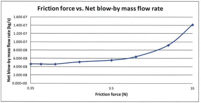
-Figure 3.2 Effect of friction force coefficient on net blow-by mass flow rate.. ...-.... 57

-Figure 3.3 Sample first stage expander model with piston inertia... 58

-Figure 3.4 First stage acceleration and velocity during intake.. ... 59

-Figure 3.5 Sample second stage expander model with piston inertia...- 60

-Figure 3.6 First stage expander model with no touchdown after 100 cycles...- 62

-Figure 3.7 Second stage expander after 100 iterations.. ...- 63

-Figure 3.8 First stage indicator diagram for low mean reservoir pressure.. ...- 66

-Figure 3.9 Second stage indicator diagram for no addition with low mean pressure...- 67

-Figure 3.10 First stage indicator diagram for early helium addition.. ...- 68

-Figure 3.11 Second stage indicator diagram for early helium addition... 68

-Figure 3.12 First stage indicator diagram for helium addition near target pressure ...- 69

-Figure 3.13 Second stage indicator diagram for helium addition near target pressure...- 70

-Figure 3.14 First stage indicator diagram after helium addition... 71

-Figure 3.15 Second stage indicator diagram after helium addition ... 71

-Figure 3.16 First stage reservoir pressures plotted over time ...- 72

-Figure 3.17 Second stage reservoir pressures plotted over time...-73

-Figure 3.18 First stage high pressure model...-75

-Figure 3.19 Second stage high pressure model...-76

-Figure 3.20 First stage helium reduction expander model...-77

-Figure 3.21 Second stage helium reduction expander model. ... 77

-Figure 3.22 First stage helium reduction normal operation... 78

(7)

-Figure 3.24 First stage reservoir pressures plotted over time ...- 80

Figure 3.25 Second stage reservoir pressures plotted over time...- 80

Figure 3.26 Indicator diagram for the switch state constants.. ...- 81

Figure 3.27 Indicator diagram for switch states when two reservoir pressures are switched. -83 Figure 3.28 The reservoir pressures plotted over time.. ...- 84

Figure 3.29 Control diagram for steady state expander operation...- 86

Figure 3.30 First cycle of expander start up.. ...- 89

Figure 3.31 Expander startup after 10 cycles...- 89

Figure 3.32 Expander startup after 20 cycles...- 90

(8)

LIST OF TABLES

Table 2.1 Reservoir Tem perature Results...- 45

-Table 3.1 Simple control scheme for expander model. ...- 61

-Table 3.2 Reservoir switch conditions for expansion and recompression...- 62

-Table 3.3 Switch states for expander operation. ...- 87

-Table B. 1 The nondimensional cutoff and recompression volumes...- 104

-Table B.2 Reservoir A pressures and corresponding recompression and cutoff volumes...- 104

-Table B.3 Reservoir B pressures and corresponding recompression and cutoff volumes...- 105

-Table B.4 Reservoir C pressures and corresponding recompression and cutoff volumes...- 106

-Table B.5 Reservoir D pressures and corresponding recompression and cutoff volumes...- 107

-Table C. 1 Assumptions applying to the pressure reservoirs...- 108

-Table C.2 Assumptions applying to the expander intake, expander exhaust, the warm volume, and the cold volum e ...- 108

(9)

-Chapter 1:

Introduction and Background

1.1 Background

NASA's future plans include long distance missions that will require the storage of cryogenic fuels (liquid oxygen and liquid hydrogen) in low earth orbit. Temperatures in low earth orbit can be as high as 250 K [1], well above the atmospheric boiling points of oxygen (90 K) and hydrogen (20 K). It becomes apparent then that the long term storage of cryogenic fuels in low earth orbit will require active cooling and management.

The modified Collins cryocooler, discussed in this work, is being developed by AMTI and MIT in response to this need. The most significant innovation in this machine over previous Collins-type machines is the use of a floating piston in the expander. The floating piston design eliminates the mechanical linkages in the expander and utilizes electronic "smart valves" for piston actuation. In previous work on this type of expander gas flow around the floating piston reduced the performance of the expander and, on occasion, contributed to the stopping of the expander's cyclic operation. In this work expander models have been developed to investigate the effects of leakage across the piston and to develop control algorithms to permit steady operation of the expander.

In what follows, the differences between the Collins cycle and the modified Collins cycle as well as the benefits of using a modified Collins machine over a traditional Collins machine are clarified. The significance of the floating piston expander design is also explained.

(10)

Additionally, previous work on the modified Collins cryocooler and the performance of the previous prototype are discussed.

1.2 The Collins Cycle

In 1946, Dr. Samuel C. Collins developed an efficient cryostat that, for the first time, produced liquid helium in a safe and cost effective manner [2]. The machine is safer because it eliminates the need to use hazardous cryogenic hydrogen as a precooling fluid. Additionally, hydrogen has a freezing point at roughly 14 Kelvin so helium is the only feasible working fluid below this temperature. The Collins liquefier uses multiple stages of heat exchangers and expanders to cool high pressure helium as shown in Figure 1.1. High pressure helium is passed through a series of heat exchangers that are in counter flow with low temperature and low pressure helium. At each expander stage, some of the helium in the high pressure line is expanded and re-circulated into the low pressure helium return. This increases the pre-cooling of

/Com

pressor

Heliu iIst _Expander

SupplyWV

2nd Expander

J-Tvalve Liquid H eliu m

(11)

the helium toward the boiling point before liquefaction is achieved. A final expansion occurs through a Joule-Thomson valve (J-T valve). Unlike nitrogen or oxygen, helium has a negative Joule-Thomson coefficient at room temperature; the temperature of the fluid increases with a

decrease in pressure at constant enthalpy. Neon and hydrogen also have negative J-T coefficients at room temperature but neon's melting point is too high for this application (24.5 K) and hydrogen is too unstable for a working fluid. The machine continues to cool and recycle the helium until the inversion temperature (45 K) is reached; at which point the J-T coefficient becomes positive. Below the inversion temperature the J-T valve can be used to liquefy the helium. A T-s diagram for the Collins liquefaction cycle is shown in Figure 1.2.

The cryocooler developed here is a modified version of this Collins machine. The J-T valve is eliminated and the machine functions as a refrigerator with the helium flow in a closed loop as shown in Figure 1.3. The key difference between this and a traditional Collins machine is that the system is designed in a modular fashion. Each cooling stage is connected to the

T

1st

Expansion

J-T

2nd

Expansion

S

Figure 1.2 Collins cycle T-s diagram

(12)

Helium Heat

Compressor

t

f

Rejection

Recuperative aHeat Exchanger Plenum 1 2nd Stage 1st Stage Expander ExpanderE 4Plenum Qtoxygen at 100 K Qhydrogen at 20 K

Figure 1.3 Modified Collins cryocooler for current design. The first stage is designed for 100 W at 100 K with a liquid oxygen based heat load and the second stage is designed for 25 W at 20 K with a liquid hydrogen based heat

load.

compressor in parallel (as opposed to the traditional Collins machine shown in Figure 1.1 where all cooling stages are connected in series) with a small pre-cooling flow from the high temperature stage to the low temperature stage. Additional stages can be added for new heat loads or to achieve lower temperatures. Segado et. al. [3] showed that adding a second expander to each stage could increase the efficiency of the machine but the increased difficulty of constructing two expanders in each stage outweighs the added benefit.

Each stage has a separate recuperative heat exchanger that, with the exception of the precooling flow from the first stage to the second stage, does not interact with any other stage.

(13)

In the first stage, helium that is exhausted from the expander is passed through a heat exchanger in contact with the liquid oxygen heat load to provide cooling. Before reaching the liquid oxygen load, a portion of the helium is bled off to the second stage recuperative heat exchanger. In the second stage, expanded helium is passed through a heat exchanger to cool the liquid hydrogen heat load. The cryocooler is designed to provide 100 Watts of cooling at 100 K to the liquid oxygen and 25 Watts of cooling at 20 K to the liquid hydrogen.

1.3 The floating piston expander

The expander utilizes a novel floating piston design, shown by the sample diagram of a single stage in Figure 1.4. A feature of this design is that there are no mechanical linkages to the

a) Heat b Helium Rejection Compressor Recuperative Heat Exchanger Plenum-Heat Load ReservoirsD_ReseroirsPA>_{PB> PC> PD:} PA B C D .ar Snvolume Reservoir valves Floating piston

Intake valve Exhaust valve

(D -1 AkD~~

rCold

volume (P _(P m=0 1 Mnn

( max L)

Figure 1.4 Expander schematic with pressure reservoir A schematic of the floating piston design for the expander.

a) A single stage of the modified Collins design. mi

(14)

piston. The piston resides inside a cylinder attached to four pressure reservoir valves, a high pressure intake valve and a low pressure exhaust valve.

From the discharge port of the compressor and after the heat exchanger used for heat rejection to the environment, high pressure helium is cooled in the recuperative heat exchanger (shown in Figure 1.3 and Figure 1.4). The cooled, high pressure helium then fills a plenum which is connected to the cylinder's cold volume. The plenum ensures a constant supply of high pressure gas in the steady state. In the operation of the expander, the motion of the piston is controlled during the expansion and recompression of the working fluid by selectively and cyclically connecting the piston-cylinder's warm volume to four pressure reservoirs (shown in Figure 1.4) while the opening and closing of the intake and exhaust valves also control the piston motion during the intake and exhaust processes, respectively. These valves allow for computer control of the expander. In the steady state, the pressures in the pressure reservoirs are distributed between the discharge pressure (1 MPa) and suction pressure (0.1 MPa) of the compressor. A more thorough description of the expander cycle can be found in Chapter 2.

A feature of the floating piston design is that there is no sliding seal between and piston

and cylinder. This is an intentional feature because a contact seal in this gap would require maintenance that is unacceptable in a space flight application. Unfortunately, this feature comes at a cost as there can be a net flow of helium around the piston during the operation of the cryocooler. This flow can disrupt or modify the pressure distribution in the pressure reservoirs. As a consequence, the control of the piston can be compromised to the point where the expander is rendered inoperable.

(15)

1.4 Previous Work

Earlier work on the floating piston expander includes Jones and Smith [4] who demonstrated the feasibility of the floating piston concept. Traum et al. [5] developed electromagnetic smart valves that operate at cryogenic temperatures. The significance of this work was that these cryogenic valves eliminated the need for mechanical actuation in the cold volume of the expander. Additionally this allowed for computer control of the valve actuation and valve timing adjustments during expander operation. Hannon et al. [6] demonstrated single stage operation of the modified Collins machine and floating piston expander. This was a smaller scale prototype designed to achieve 1 Watt of cooling at 10 K. The prototype demonstrated cooling to 60 K with the single stage as well as cooling to 20 K with a precooling flow to simulate the first stage expander. In their initial measurements, Hannon et al. found that there was leakage past the piston between the warm and cold volumes (blow-by), and, as a consequence, the pressures in the reservoirs would slowly decrease to a point where the piston could not be moved in the necessary way. Their solution was to add a small bleed flow into the high-pressure reservoir from the discharge port of the cycle's compressor and a similar bleed from the low-pressure reservoir to the suction port of the cycle's compressor (shown in Figure 1.5).

(16)

Reservoirs

A B C D

PA >PB C PD

Compressor PA PB PC PD Compressor

discharge bleed line suction bleed

throttle line throttle

Warm volume Reservoir

valves

Floating piston

Figure 1.5 Expander used by Hannon et al with bleed line throttles

1.5 Motivation

The bleed lines implemented by Hannon et al. improved expander operation by stabilizing the reservoir pressures at levels that would allow the expander to operate. Unfortunately, the bleed lines did not eliminate the problem of blow-by from the warm volume to the cold volume past the piston. The introduction of a bleed flow into the reservoirs can augment the flow between the warm end and cold end of the piston and, as a consequence, increase the heat load to the cold volume of the expander. In addition, the flow through the two bleed valves is a parasitic flow from the discharge port to the suction port of the compressor which does not provide any additional refrigeration effect. An improved design of this expander then, is to eliminate the need for a bleed flow through the implementation of a better expander control algorithm that maintains a net zero mass flow past the piston in the steady state.

(17)

1.6 About this thesis

To this end, this thesis describes work on a model designed to understand the effects of a control algorithm on the long-term pressure distribution of the pressure reservoirs in the cryocooler. An initial model is developed to determine the dependence of expander operation on various control parameters. The model is then extended by using the piston inertia to predict the helium flow through the gap. The piston control scheme uses the new piston-inertia based model to accurately predict helium blow-by and maintain a net zero flow in the steady state.

(18)

Chapter 2:

Expander Modeling

A thermodynamic model for the expander is developed here to explore the effect of

various control parameters on the performance of the expander. This model allows a direct investigation of valve timings on the mass flows between and the pressure distributions of the pressure reservoirs. From this model a performance map can be created for controlling the motion of the floating piston.

2.1 Expander Cycle Description

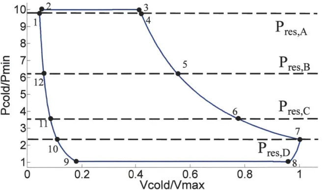
The targeted (ideal) cycle for the expander is shown in Figure 2.1 as a non-dimensional indicator diagram. The abscissa of this plot is the cold volume, normalized by the maximum volume; whereas, the ordinate is the cold volume pressure normalized to the compressor suction pressure. The steady state pressures of the reservoirs are also indicated as dashed lines.

The cycle begins in state 1 where the cold volume pressure is equal to the pressure in reservoir A and the cold volume is at a minimum. In state 1, the intake valve, exhaust valve, and all reservoir valves are closed.

(19)

res,A

S7-res,B

~

12---0

5-0

_P

CL

4 -6

res,C

3 -n

3- 7

2~

10 _P

res,D

1- 9 I so,

0

0.2

0.4

0.6

0.8

1 VcoldNmax

Figure 2.1 Expander cycle dimensionless indicator diagram. The normalized pressure versus the normalized volume is plotted for each state. The horizontal dotted lines represent the steady state pressures of each reservoir (Pmin = 100 kPa, Vma= 0.1 liters).

As part of the blow-in process, the intake valve opens and high pressure helium flows through the intake valve into the cold volume. The pressure in the cold volume rises and forces the piston up toward the warm volume until the cylinder pressure is equalized with the intake pressure at state 2.

At state 2 the intake process begins, the intake valve remains open and the reservoir A valve opens. Due to the pressure difference across the reservoir A valve, helium from the warm volume begins to fill reservoir A and the piston continues to advance into the warm volume. As the piston advances, more high pressure helium is drawn into the cold volume through the intake valve until the piston reaches the predetermined cutoff volume (Veo) and the intake valve closes (state 3).

(20)

The expansion process begins with the closing of the intake valve. Gas continues to flow into reservoir A and the helium in the cold volume expands until the pressure in the warm volume matches the pressure in reservoir A (state 4) when the reservoir A valve closes. This is immediately followed with the opening of the reservoir B valve so that the expansion process is continued. The gas in the cold volume continues to expand as the helium from the warm volume flows into reservoir B until the pressure in the warm volume matches the pressure in reservoir B (state 5). At this point the reservoir B valve closes and the reservoir C valve opens. The cold volume helium expansion continues as the gas from the warm volume flows into reservoir C until the pressure in the warm volume matches the pressure in the reservoir (state 6). At this point the reservoir C valve closes and the reservoir D valve opens. The cold volume gas continues to expand as the helium from the warm volume flows into reservoir D until the pressure in the warm volume matches the pressure in the reservoir or until the maximum cold

volume is reached (state 7). At this point the reservoir D valve closes.

All valves are closed at state 7. The exhaust valve opens beginning the blow-out process

where the helium from the cold volume flows out of the cylinder through the exhaust valve. The gas in the warm volume expands as the piston moves toward the cold volume. The pressure in the cold volume continues to decrease until the cold volume pressure matches the exhaust pressure of the expander (state 8), ideally the compressor suction pressure.

In the exhaust process, from state 8 to state 9, the exhaust valve remains open and the reservoir D valve opens. Since the pressure in reservoir D is greater than the expander exhaust pressure, helium from reservoir D fills the warm volume and the piston advances into the cold volume. As the piston advances, more low pressure helium is forced out of the cold volume

(21)

through the exhaust valve until the piston reaches the predetermined recompression volume

(Vrec) and the exhaust valve closes (state 9).

The closing of the exhaust valve at state 9 initiates the recompression process. The helium in reservoir D continues to fill the warm volume, compressing the helium in the cold volume until the pressure in the warm volume matches the pressure in reservoir D (state 10) when the reservoir D valve closes and the reservoir C valve opens. Gas from reservoir C fills the warm volume compressing the helium in the cold volume as the piston moves into the cold volume. When the pressure in the warm volume matches the pressure in reservoir C (state 11), the reservoir C valve closes and the reservoir B valve opens. Gas from reservoir B now fills the warm volume continuing the cold volume gas compression as the piston moves into the cold end of the cylinder. When the pressure in the warm volume matches the pressure in reservoir B (state 12), the reservoir B valve closes and the reservoir A valve opens. Gas from reservoir A fills the warm volume compressing the helium in the cold volume until the pressure in the warm volume matches the pressure in reservoir A (state 1), when the reservoir A valve closes and the cycle is complete.

2.2 Development of an ideal model for each process

The cycle was modeled to understand expander behavior as a function of the cutoff and recompression volumes. In this model the cylinder and piston are assumed to be adiabatic while the gas in the reservoirs is assumed to remain at constant temperature. Mass flow through the piston-cylinder gap is assumed to be zero in this model. As a consequence, the total mass in the reservoirs and the warm volume remains fixed in this model. This total mass is set by setting each reservoir volume, pressure, and temperature to fixed values (5 liters, 500 kPa, and 300 K,

(22)

respectively) at the beginning of the simulation. Additional assumptions made in this model are tabulated in Appendix C.

The reservoir, intake, and exhaust valves were each modeled with fixed flow resistances so that the mass flow rate through each valve was the product of its flow resistance and the pressure drop across the valve. The piston mass in this model is set to zero so that the pressures in the cold and warm volumes are always equal and the entire cylinder is at uniform pressure. In each process the work done by the gas in one volume on the floating piston is assumed to be equal to the work done on the gas by the floating piston in the other volume. Helium is modeled as an ideal gas.

In the blow-in process (states 1 to 2), the initial pressure (state 1) in the cold volume (Pcold) is the high pressure reservoir pressure (PA). The intake valve opens and the mass flow

through the valve is determined as the product of the valves flow resistance and the pressure difference across the valve,

rnvalve = Kvalve (APvaive) (2.1)

where Kvaive is the flow resistance of the valve and APvalve is the pressure difference across the valve. The process is then modeled using the First Law for an open system with a control volume enclosing all of the gas in cylinder. Due to the zero piston mass assumption the pressure is equal on either side of the piston and all helium within the cylinder can be modeled at a uniform pressure.

The First Law for an open system: dEcv

dt = - V + (rIh)in - (inh)out (2.2)

(23)

where E, is the energy state of the gas in the control volume and h is the enthalpy of the gas carried across the control volume boundary. In this case there is no mass flow (1h) out of the control volume and the cylinder is assumed adiabatic therefore the heat transfer into the control volume (Q) is zero. There is also no work (W) because the cylinder volume is fixed. Assuming perfect mixing in the cold volume, the First Law for the cold volume is re-written as

d(mcVT)c.ld = (Kintake(Fintake - Pc)CpTintake) _(2.3)

dt i

where Kintake is the intake valve flow resistance, Pintaje is the compressor discharge pressure, Pc is the pressure in the cold volume, Tintake is the temperature of the intake gas, c, is the specific heat of helium at constant volume and c, is the specific heat of helium at constant pressure. Since the temperature is not uniform in the cylinder (temperatures differ between the warm and cold volume), the ideal gas assumption is used to manipulate the left hand side of equation 2.3 for the uniform pressure in the cylinder (due to the zero mass piston assumption). The result is

1 d(PcVtot) ( ₂₄

y - 1 dt =

(Kintake(Pintake

- Pc)CpTintake)in9

where Vtot is the volume of the cylinder and y is the ratio of the specific heat at constant pressure and the specific heat at constant volume (1.66 for helium). Since the total volume of the cylinder is fixed it can be pulled out of the differential. Separating the differential and integrating with a fixed time step results in the next pressure state of the cylinder.

Separating the differential equation 2.4:

Vtot (dPc) = (Kintake(Pintake - Pc)cpTintake). dt _(2.5)

Descritizing for the fixed time step during integration:

APc = v (Kintake(Pintake - Pc)CpTintake)intstep (2.6)

(24)

Solving for the new pressure state:

Pc,2 = Pc,1 + (Kintake(intake - Pc)CpTintake)intstep (2.7)

Vtot

where tstp is the fixed time step used to numerically integrate each process throughout the cycle. Since the piston is assumed massless, this new pressure is the pressure in both the warm and cold volumes. The displacement of the piston is then determined by assuming that the gas in the warm volume undergoes an isentropic compression.

Applying the Second Law to the warm volume,

dS = cV In (w,2 + cp ln (Vw2 = 0 (2.8)

and simplifying, the volume can be related to the new pressure as

(Vw,2)

_\VW,1 = (p _\ _{w,1 iw,} P = ₂

yCV/C

(2.9)

Vw,I and Pw,I refer to the initial state of the gas in the warm volume while Vw,2 and Pw,2 refer to

the state of the gas in the warm volume after the time step. The new volume of gas in the cold volume is Vc,2 = Ytot - Vw,2 and the new helium temperature is found using the ideal gas

assumption.

The intake process (process 2-3) is modeled using the same control volume as the blow-in process (process 1-2). In this case, however, there is now helium flowblow-ing from the warm volume into reservoir A. Writing the First Law for the cylinder

dEcv =

nh)n

- (ihh)out

(2.10) dt

where the enthalpy flow rate through the cold valve, (riih)in, is

(25)

and the enthalpy flow rate from the warm volume into reservoir A, (rih)out, is

(rhh)out = Kres,A(Pw - Pres,A)CPTW (2.12)

where Kres,A is the flow resistance through the valve connecting the warm volume to reservoir A,

Pres,A is the helium pressure in reservoir A. The temperature of the helium remaining in the

warm volume, Tw, is assumed to be constant. This comes from modeling the mass remaining in the warm volume with no entropy generation

dS

=

c In

(w3)

-

R In

(')

=

0 (2.13)

Tw,2 \ w,2/

where R is the ideal gas constant. During intake (process 2-3), the pressure is constant at the intake pressure, therefore the temperature of the gas in the warm volume must remain constant to satisfy equation 2.13. The new piston position is determined using the First Law for each volume. The First Law for the cold volume is

dEcv_

dt =

-W

ec

+ (ihh) ;u (2.14)

where

Wc

is the work done by the gas in the cold volume. This work is determined by setting the work done by the gas in the cold volume equal to the work done on the gas, by the piston, in the warm volume. The First Law for the warm volume is

dEcv_

dt - N , - (rhh)out (2.15)

where

W,

is the work done on the gas in the warm volume. Simplifying the left hand side (recall T, is fixed during intake) and solving for the work gives

dm~

-N, = (rhh)out + cTw dt. (2.16)

(26)

Substituting equation 2.16 into equation 2.14 and using the ideal gas law on the left hand side of equation 2.14 gives

1 d(PcVc) ₌_-c_PV dmW_d _{+ (rhh);n}_- _(ihh)out. _(2.17)

y -1 dt dt

When equation 2.17 is integrating for the fixed time step, the equation is solved for the new cold volume

Vc,3 = p [Pc,2Vc,2 + (y - 1)(-cvTw(m 3,w - m2,w)+(rhh)intstep - (ihh)outtstep].

c,3

(2.18)

Each expansion process (process 3-4, process 4-5, process 5-6, and process 6-7) is modeled in a manner similar to blow-in. The difference between the blow-in and expansion processes is that helium is only flowing out of the warm volume into each reservoir and there is no flow into the cold volume. The fixed mass in the cold volume is modeled with no entropy generation. The First Law for the entire cylinder volume with no work (zero displacement) and no heat transfer (adiabatic) is

dE~_

dc = -(rhh)out _(2.19)

dt where

(ih)out = Kres(Pw,3 - Pres)CpTw,3 (2.20)

and Kres is the flow resistance of the open reservoir valve, Pw,3 is the initial pressure in the warm volume, Pres is the pressure in the reservoir, and T,,3 is the initial temperature of the warm

volume. The First Law result is similar to that of the blow-in and the new warm volume pressure is defined as

w,4 - rw - 1_-(.1

Pw,4 = Pw,3 - (Kres(Pw,3 - Pres)CpTw,3)tstep. (2.21)

(27)

Since the pressure is equal across the piston and the gas in the cold volume is assumed to expand with no entropy generation, the Second Law gives the new piston position with

V cPc,4c pc,3 (2.22)

k

c,

3 )

C,3

c,4

where Ve,3 and P,,3 refer to the initial volume and pressure of the gas in the cold volume while Ve,4 and P,,4 refer to the state of the gas in the cold volume following the time step.

The blow-out process (process 7-8) is modeled in a manner very similar to the blow-in process with the only difference being the flow direction. During blow-out the cool, low pressure helium flows out of the cold volume through the exhaust valve. The warm volume is modeled as an isentropic expansion.

The exhaust process (process 8-9) is similar to the intake process. The differences are that helium flows out of the cold volume (cold volume helium temperature is modeled as constant with no entropy generation assumed for the gas remaining in the cold volume) and that helium flows into the warm volume from reservoir D. The work done by the gas in the warm volume on the piston is reflected as the work done by the piston on the gas in the cold volume as well.

Each recompression process (process 9-10, process 10-11, process 11-12, and process

12-1) is modeled as a reversible compression in the cold volume and an open system for the entire

cylinder with helium flow out of each reservoir into the warm volume. A complete list of the model for all processes in the expander cycle can be found in Appendix A.

2.3 Cutoff and Recompression volume study

In the expander control model the cutoff volume Voo, which corresponds to the state 3 volume in Figure 2.1, and the recompression volume Vrec, which corresponds to the state 9

(28)

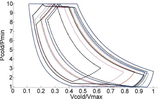
volume in Figure 2.1, are chosen fixed points in the cycle. They mark the end of the intake process and the end of the exhaust process, respectively. Increasing the intake stroke (increased Voo) will increase the total helium mass in the cold volume. The larger volume of gas in the cold volume raises the likelihood that during expansion, with less distance for the piston to travel to reach the top of the cylinder and more gas for expansion, the piston will touch down on the top of the cylinder. When the piston dwells on the top or the bottom of the cylinder, mass flow through the piston cylinder gap increases due to the increased pressure difference across the piston. Hence, when the piston dwells at the top of the cylinder, gas from the cold volume will flow up into the warm volume to add mass to the reservoirs in the case that the total mass in the reservoirs is too low. Similarly, a longer exhaust stroke (reduced Vrec) will reduce the total mass in the cold volume. A smaller volume of gas in the cold volume raises the likelihood that during recompression, with less distance for the piston to travel to reach the bottom of the cylinder and less gas for recompression, the piston will touch down on the bottom of the cylinder. With the piston dwelling on the bottom of the cylinder, the pressure difference across the piston will increase blow-by from the warm volume to the cold volume to remove mass from the reservoirs in the case that the total mass in the reservoirs is too high. The model discussed in the previous section was run with varying cutoff and recompression volumes to see what the impact was on the shape of a steady state cycle. A sampling of stable cycles with a large P-V span as

determined by the simulation is shown in Figure 2.2. A good (or ideal) cycle is defined as those that close with a large swept volume (roughly 90% of Vmax or greater).

These plots suggest that the ranges of acceptable cutoff and recompression volumes are limited. The suggested values for the normalized cutoff volume can vary only from 0.33 to 0.5 whereas the values for the normalized recompression volumes

(29)

Cutoffvolume range

- 5 E % .4%%% 6 .4 % % \ .% .% % %2. % %% %%%4

o

\End of

C

-

%%

%4 Nansion 3 %\ % % % % Recompression

2-1

\

%%..olume

range

(j --- --- t.4' O

0 ---

--

-fr420.

0.6

0.81 Vcold/Vmax

Figure 2.2 Ideal Expander Cycle Samples. The normalized pressure versus normalized volume diagrams

for various cutoff and recompression volumes are plotted for the cold volume gas (Pma = 100 kPa, Vm, = 0.1

liters).

can vary from 0 to 0.5. If the simulation is run with values outside of this range, the cycles degenerate into cycles that do not span the entire range of available volumes or pressures. Figure

2.3 is a sample of indicator diagrams for cycles in which the recompression volumes are chosen

to be too large. In this case, the large recompression volume ends the exhaust stroke so early that a large portion of the gas that was cooled during expansion is recompressed instead of being exhausted, thus reducing the cooling power of the expander. As a result, the piston resides primarily in the warm volume throughout the cycle. Figure 2.4 is a sample of indicator diagrams for cycles in which the cutoff volumes are too low. The shortened intake stroke reduces the mass in the cold volume and consequently the gas is expanded without taking full advantage of the maximum volume in the cylinder. This results in a piston that resides primarily in the cold end of the expander throughout the cycle, thereby reducing the total cooling.

(30)

6- 1 \ % - 5 . 4 3-

2-0

0.1 0.2 0.3 0.4 0.5 0.6 0.7 0.8 0.9

1 VcoldNmax

Figure 2.3 High Vee expander cycle samples. The normalized pressure versus the normalized volume diagrams for various cutoff and recompression volumes are plotted for the cold volume gas. In this sample all of the recompression volumes are too large and the maximum swept volume of the expander is not achieved (Pmm=100 kPa, Vm&=O. 1 liters).

10-

9-

8-.C7

E

o.6-1

-o

5-0 4- 3-

2-0

0.1

0.2

0.3 0.4 0.5

0.6

0.7

0.8

0.9

1 VcoldNmax

Figure 2.4 Low Ve, expander cycle samples. The normalized pressure versus the normalized volume diagrams for various cutoff and recompression volumes are plotted for the cold volume gas. In this sample all of the cutoff volumes are too small and the maximum swept volume of the expander is not achieved (Pmin=100 kPa, Vma=O. liters).

(31)

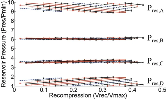
The steady state pressures that are attained by each of the reservoirs as a function of recompression and cutoff volumes are shown in Figures 2.5 and 2.6. More specifically, Figure 2.5 is a plot of the normalized reservoir pressures as a function of a normalized cutoff volume (Vco). Each line in Figure 2.5 corresponds to a specific and fixed recompression volume. Similarly, Figure 2.6 is a plot of the normalized reservoir pressures as a function of the normalized recompression volume (Vree). Each line in Figure 2.6 corresponds to a specific and fixed cutoff volume. Both plots represent a collection of cycles that close and operate smoothly. In both plots, the variations of the pressure in the high and low pressure reservoirs are larger than the variation in the intermediate reservoirs which is consistent with the observed performance of previous prototypes [7]. Therefore, given that the maximum and minimum pressures are 1 MPa and 0.1 MPa respectively, it can be expected that reservoir B and reservoir C will settle to

9 p-res,A

8-6 - res,B CO)

C 5

CL 4

4L

pres,C

0

3-0 2-

_pe,

(3

0.35

0.4

0.45

0.5 Cutoff (VcoNmax)

Figure 2.5 Reservoir pressure vs. cutoff volume. The normalized reservoir pressures for a fixed recompression volume are displayed as a function of the normalized cutoff volume (Pmin = 100 kPa, Vm, = 0.1 liters).

(32)

1 9res,A

CL) c 5-a)

-4

.

6 -

_PresBc

Lo -4-P

2 3res,C

~

I

.... -...- 4 PresP

0

0.1

0.2

0.3

0.4

0.5 Recompression (VrecNmax)

Figure 2.6 Reservoir pressure vs. recompression volume. The normalized reservoir pressures for a fixed cutoff volume are displayed as a function of the normalized recompression volume (Pmin = 100 kPa, Vma = 0.1 liters).

approximate pressures of 600 kPa and 350 kPa regardless of the cutoff and recompression volumes selected. The numerical results shown in Figure 2.5 and Figure 2.6 are tabulated in Appendix B. The cutoff and recompression volumes for the indicator diagrams shown in Figure

2.2 are also tabulated in Appendix B.

The sensitivity of the low pressure reservoir (D) to the recompression volume can be understood by considering the specifics of the intake and discharge processes to that reservoir. In steady state the mass flow into reservoir D occurs during process 6-7 in Figure 2.1; whereas the mass flow out of reservoir D occurs during processes 8-9-10. If the recompression volume is increased slightly (state 9 is moved to the right in Figure 2.1) the mass flow out of reservoir D is reduced. As a consequence, mass begins to accrue in reservoir D and the pressure in reservoir D slowly increases over many cycles. As the pressure rises in reservoir D the volume of state 10

(33)

decreases which, in turn, increases the net mass flow out of reservoir D. The increased pressure in reservoir D also reduces the net mass flow into reservoir D during process 6-7. These changes in the net mass flow act as a negative feedback to drive the reservoir pressure to a new equilibrium where the mass flow into reservoir D during expansion is equal to the mass flow out of reservoir D during exhaust and the first recompression.

Analogously, the sensitivity of the high pressure reservoir (A) to the cutoff volume can be understood by considering the specifics of the intake and discharge processes to that reservoir. In steady state the mass flow into reservoir A occurs during processes 2-3-4 in Figure 2.1; whereas the mass flow out of reservoir A occurs during process 12-1. If the cutoff volume is

decreased slightly (state 3 is moved to the left in Figure 2.1) the mass flow into reservoir A is reduced. As a consequence, the mass in reservoir A and hence the pressure in reservoir A slowly decreases over many cycles. As the pressure decreases in reservoir A the volume of state 4 increases which, in turn, increases the net mass flow into of reservoir A. The reduced pressure in reservoir A also results in a reduced mass flow out of reservoir A during process 12-1. These changes in the net mass flow act as a negative feedback to drive the reservoir A pressure to a new equilibrium where the net mass flow into and out of the reservoir is equal.

The intermediate pressure reservoirs (reservoirs B and C) are less sensitive to changes in the cutoff and recompression volumes because the mass flow in and out of these reservoirs are not directly tied to the length of the intake and exhaust strokes. No mass flow into or out of the reservoirs takes places at constant pressure as observed with reservoirs A and D. Any change in the mass flow into the reservoir during expansion is reflected as a change in mass flow out of the reservoir during recompression. This reflection stabilizes the pressure in both of the intermediate

(34)

reservoirs. As a result, only the volumes at which the reservoir B and reservoir C valves open and close change with new cutoff and recompression volumes but the pressures do not.

2.4 Total warm helium mass study

The analysis above fixed the mass in reservoirs such that the average pressure ratio (Paverage/Pmin where Pmin =100 kPa) of the reservoirs was 5.0. The impact of the average pressure ratio on the steady state reservoir pressures for the expander was modeled by running simulations with different average reservoir pressures. Figure 2.7 shows the steady state reservoir pressures as a function of the average reservoir pressure ratio ranging from 1.5 to 8.0 for three different cutoff and recompression volumes. The steady state pressure in reservoir A monotonically

10 PresA-9 8

S

7 .-- ~resB.---.--- 6 -~4 4e, 2 -res,D) 1.5 2.5 3.5 4.5 5.5 6.5 7.5

Paverage/Pmin

Vco/Vmax , Vrec/Vmax _{-0.405, 0.255 -- 0.462, 0.340 ---0.371, 0.127}

Figure 2.7 Average reservoir pressure vs. steady state reservoir pressure. The normalized reservoir pressures versus the normalized average reservoir pressures are plotted for three cutoff and recompression volumes (Pm. =

(35)

increases with the average pressure and then saturates at the compressor discharge pressure for average reservoir pressures above 5.5. Similarly the reservoir D pressure is fixed at the compressor suction pressure up to an average reservoir pressure of roughly 4. The reservoir D pressure then monotonically increases with average pressure above 4. The pressures for the intermediate reservoirs show no such saturation behavior for the ranges shown in Figure 2.7. The simulations show that for good control of the piston motion, the distribution of pressures in the pressure reservoirs would, ideally, be distributed evenly between the compressor discharge

and suction pressures in the machine. In Figure 2.7 this distribution occurs when the average pressure ratio for the reservoirs is between 4.5 and 5.5.

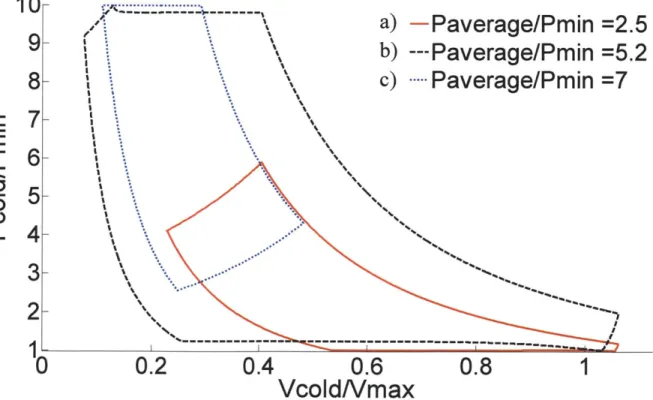
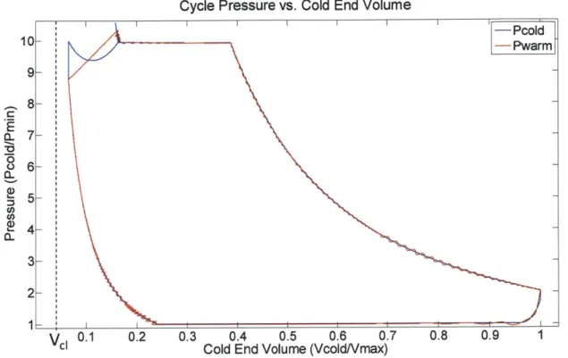
Figure 2.7 shows reservoir pressure distributions for cycles that closed. Some of these cycles, however, did not sweep the entire available volume or pressure ranges. For example, the three cycles shown in Figure 2.8 correspond to normalized average pressures of 2.5, 5.2, and 7 (the normalized cutoff and recompression volumes for the cycles shown in Figure 2.8 are 0.405 and 0.255, respectively). In the case when the normalized average pressure is 2.5, due to the lower reservoir pressures, the piston is forced to reside in the warm end of the cylinder throughout the cycle. In the case when the normalized average pressure is 7, due to the higher reservoir pressures, the piston is forced to reside in the cold end of the cylinder throughout the cycle. In the case when the normalized average pressure is 5.2, the cycle spans the entire P-V space maximizing the work per cycle and hence the cooling power per cycle. This cycle is in the ideal range suggested earlier. The three dotted vertical lines in Figure 2.7 correspond to the three cycles shown in Figure 2.8. In retrospect these results are not surprising when the extreme limits are considered. In the case of an infinite initial pressure in the reservoirs, the high pressures in the reservoirs drive and hold the piston to the cold end of the cylinder throughout the cycle. In

(36)

the zero initial pressure limit, the piston is forced to the top of the cylinder by both the compressor discharge and suction pressures in the cold volume throughout the cycle. In either of these extreme cases the piston is immobile.

Although the model assumes there is no leakage past the piston, the results of Figure 2.7 and Figure 2.8 can be used to determine the expected behavior of the floating piston expander with a small leak across the piston. A net average flow of helium from the warm volume to the cold volume will decrease the mass (and pressure) in the reservoirs. The average pressure in the reservoirs will decrease and the pressure distribution of the reservoirs will begin to concentrate towards the minimum pressure in the expander (as shown in Figure 2.7 for values of Paverage/Pmin< 4.0). The cycle the expander executes will be restricted only to larger cold volumes

10 a)

-Paverage/Pmin =2.5

9 _{b) --- Paverage/Pmin =5.2}

8 c)

Paverage/Pmin

=7

E

a

6

-5 0

Q4-

3-2

-- - --- - --- --1 0 0 0.2 0.4 0.6 0.8 1 VcoldNmax

Figure 2.8 Average pressure indicator diagrams. The resultant normalized indicator diagrams for the varying

average pressure (Pmin = 100 kPa, Vmax= 0.1 liters). a) A cycle with an average reservoir pressure that is too small.

b) A cycle with an average reservoir pressure that allows the full cycle to occur (ideal range). c) A cycle with an

(37)

and lower pressure as shown by the red (Paverage/Pmin = 2.5) cycle in Figure 2.8. A net average flow of helium from the cold volume to the warm volume would increase the mass (and pressure) in the reservoirs. The average pressure in the reservoirs will increase and the pressure distribution of the reservoirs will begin to concentrate towards the maximum pressure in the expander (as shown in Figure 2.7 for values of Paverage/Pmin> 5.5). The cycle the expander executes will be restricted only to smaller cold volumes and higher pressures as shown by the blue (PaveragelPmin = 7) cycle in Figure 2.8.

The model used up to this point depicts the performance of an idealized expander. For integrating these results into a physical prototype, some of these idealizations must be reconsidered. However, the conclusions of this study remain valuable for predicting expander behavior. In what follows here and in Chapter 3, the model is augmented to include more accurate flow characteristics for the intake, exhaust, and reservoir valves. Additionally, the sizes of the reservoirs used up to this point are quite large (5 liters per reservoir). In fact, the study here shows that significantly smaller reservoirs can be used.

2.5 Valve Flow

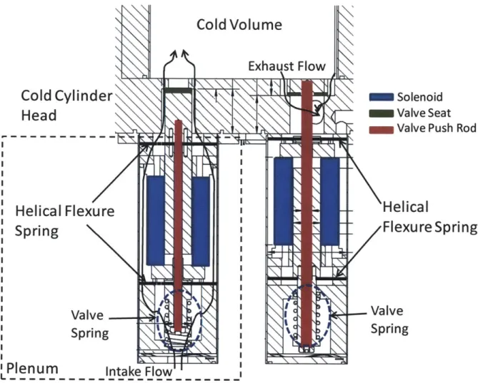
The K values used for the impedances of the valves in the study above were arbitrarily assigned and adjusted to make the operating frequency of the expander 1 Hz. These valves can be better approximated to the actual values by considering the simplified drawing of the valve design shown in Figure 2.9. The intake valve is mounted on the cold cylinder head inside a pressurized plenum. In Figure 1.3 the plenum sits between the intake valve and the high pressure side of the recuperative heat exchanger. In the physical cryocooler the intake valve is mounted directly in the plenum and the intake flow passes through the entire valve assembly as shown in Figure 2.9. The plenum acts as a pressure stabilizer for the flow to the intake port. The exhaust

(38)

Cold Cylinder

Solenoid

Head Valve Seat

Valve Push Rod

Helical

Flexure

Helical

Spring

Flexure Spring

Valv .---

--...Valve

gSpring

Plenum

Intake Flow

Figure 2.9 Cold Valve Schematics. When activated, the high pressure intake valve (left) pulls down from the seat and the low pressure exhaust valve (right) pushes up into the cold volume.

valve is mounted directly to the exhaust port of the cold cylinder head. The exhaust gas flows out through a port just below the valve seat. In both valves, current is supplied to the solenoid, pushing the valve rod against the spring force (the force that normally holds the valve closed).

To get a better prediction of the helium flow through the intake and exhaust valves. The valves were modeled by assuming that the helium was incompressible through the duct for the small, fixed time step. Minor losses were taken into account as well. The state of the gas downstream of the valve is adjusted for every time step. In the case that the pressure ratio across

(39)

the valve exceeds that of the critical pressure ratio, then the mass rate flow through the valve is determined based on the critical pressure ratio. White [8] defines the critical pressure ratio as

P*critical =

(

2

1/Yl

(2.23)

where y is the specific heat ratio for helium (1.66). The critical pressure ratio for helium is

0.488. Consequently, the helium mass flow rate through the valve is never greater than the mass

flow rate achieved by this critical pressure ratio. With the correct pressure ratio, the helium flow through the intake and exhaust valves, is

P 2 P 2

+

v

= + 2

+hf+Ehm

_(2.24)

pg 2g pg 2g

where Pi and P2 are the upstream and downstream pressures, respectively. Vi and V2 are the upstream helium velocity (assumed to be zero) and the downstream helium velocity, respectively. The variable g is the gravitational constant, p is the instantaneous helium density, hf is the head loss due to friction and Zhm is sum of the minor losses in the valve. Additionally,

hf + Ehm - -- + EK (2.25)

2 g ( Dh

where

f

is the friction factor through the valve opening, L is the length of the valve opening, Dh

is the hydraulic diameter of the pipe and JK is the sum of the loss coefficients for each valve. With

f

<< 1 and L/Dh<l in each valve,

f

L/Dh is assumed to be negligible. Therefore,

substituting equation 2.25 into equation 2.24, the resulting flow equation is

V 2(P

1

-

P2)

G

1 ) (2.26)

(40)

The valves that will connect between the warm volume and each reservoir are purchased off the shelf and have a rated flow coefficient (Cv) of 0.210. The flow through these valves is determined using the formulas provided by Gems Sensors and Controls [9]. If P2 > 0.5P,

V Cv= (P12 - P2 2₎ (2.27) 605 F (SG) T or if P2< 0.5P1, V cv= ₁ (2.28) 13.61 P1 (SG) T

Where V is the gas velocity through the valve, P1 is the upstream gas pressure, P2 is the downstream gas pressure, SG is the specific gravity of the gas (compared to air density at STP), and T is the gas temperature.

Equations 2.26, 2.27, and 2.28 are added to the expander model described in section 2.2. Instead of using an equivalent flow resistance for each valve, the total helium flow through each valve over the fixed time period is determined. The resulting impedance of the real valves is much smaller than that of the valves from the previous study. However, because each reservoir valve has the ability to be throttled, the flow through the valve can be adjusted to slow down the expander operating frequency. With the each reservoir valve throttle down to roughly 35% of its fully open flow rate, the expander again operates in the 1 Hz to 2 Hz range with behavior similar to the previous study. This updated valve flow model is then incorporated into the First and Second Law equations for each process. It is important to use the accurate model for the valve flow because, when blow-by is considered, the valve flow will impact the dynamics of the piston

(41)

motion. The piston motion produces a pressure difference across the piston that drives the

blow-by flow.

2.6 Reservoir Volume Size

In the model described above the volume of each reservoir was assumed to be five liters; a value that is far too large to be practical in the real device. The question becomes then, how small can the volumes of the reservoirs be made and still achieve the desirable performance found in that model?

One of the simplifications that the large reservoir assumption affords is that the surface area of the reservoir is large and hence the heat transfer to the environment is large. Any dissipation that occurs in these reservoirs is immediately dissipated to the environment, keeping the temperature of the gas in the reservoir constant and near the assumed environmental temperature of 300 K. As the reservoir volume is reduced, the work dissipated in the gas in the reservoir is (roughly) the same as that of the large reservoir. Since the heat transfer rate is proportional to the surface area and the temperature of the reservoir, it is expected that the average temperature of the gas in the reservoir will increase as the surface area (volume) of the reservoir is reduced. More explicitly, the heat transfer is

Q

= heffAsurf(Treservoir - Tambient) (2.29)

where heff is the effective heat transfer coefficient, Asurf is the surface area of each reservoir, Treservoir is the average gas reservoir temperature and Tambient is ambient temperature; solving for Treservoir gives shows an estimated 20 K temperature difference.

_ Q

Treservoir - + Tambient- (2.30)

heffAsurf

To approximate the reservoir temperature, heff is assumed to be 20 W/m2-K due to natural convection and radiation, Asurf is estimated from a 1 liter cube, and Tambient is set to 300 K. The

(42)

total energy dissipated in the reservoirs is roughly equal to the cooling power (100 W) of the cryocooler. Presuming that this dissipated energy is evenly distributed across all four reservoirs,

Q

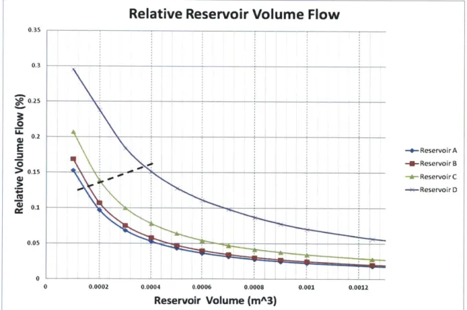
is set to 25 Watts for each reservoir. Substituting these values into equation 2.30, the temperature of the reservoir is approximately 320 K, or 20 K above ambient temperature. Every reservoir temperature was therefore set at 320 K and treated as isothermal for this updated expander model used to determine the reservoir sizes. Each reservoir was set to the same volume and the expander model was cycled with a fixed cutoff and recompression volume selected from the results shown in Figure 2.5 and Figure 2.6. The reservoir volume size was reduced until the P-V span in the steady state began to diminish. In Figure 2.10 the reservoir size

Relative Reservoir Volume Flow

0.35 0.3 0.25 0 LL _0. E --- Reservoir A -A- Reservoir B +Reservoir C -i+-Reservoir D 4) 0.1 _ _ _ 0 0 0.0002 0.0004 0.0006 0.0008 0.001 0.0012

Reservoir Volume (mA3)

Figure 2.10 Reservoir Volume Flow. The x-axis represents the volume of each pressure reservoir and the y-axis

represents the helium volume flow in each reservoir as a percentage of the total helium volume in each reservoir. The data points at 0.0001 m3

are cases that resulted in a diminished P-V span. The dotted line represents the smallest combination of reservoir volumes.

Development of a floating piston expander control algorithm for a Collins-type cryocooler