Technical Note: Impact of nonlinearity on changing the a priori of trace gas profiles estimates from the Tropospheric Emission Spectrometer (TES)

(1)

HAL Id: hal-00303267

https://hal.archives-ouvertes.fr/hal-00303267

Submitted on 25 Jan 2008

HAL is a multi-disciplinary open access

archive for the deposit and dissemination of sci-entific research documents, whether they are pub-lished or not. The documents may come from teaching and research institutions in France or abroad, or from public or private research centers.

L’archive ouverte pluridisciplinaire HAL, est destinée au dépôt et à la diffusion de documents scientifiques de niveau recherche, publiés ou non, émanant des établissements d’enseignement et de recherche français ou étrangers, des laboratoires publics ou privés.

Technical Note: Impact of nonlinearity on changing the

a priori of trace gas profiles estimates from the

Tropospheric Emission Spectrometer (TES)

S. S. Kulawik, K. W. Bowman, M. Luo, C. D. Rodgers, L. Jourdain

To cite this version:

S. S. Kulawik, K. W. Bowman, M. Luo, C. D. Rodgers, L. Jourdain. Technical Note: Impact of nonlinearity on changing the a priori of trace gas profiles estimates from the Tropospheric Emission Spectrometer (TES). Atmospheric Chemistry and Physics Discussions, European Geosciences Union, 2008, 8 (1), pp.1261-1289. �hal-00303267�

(2)

ACPD

8, 1261–1289, 2008

Linearly exchanging the prior vector for

TES estimates S. Kulawik et al. Title Page Abstract Introduction Conclusions References Tables Figures ◭ ◮ ◭ ◮ Back Close

Full Screen / Esc

Printer-friendly Version Interactive Discussion Atmos. Chem. Phys. Discuss., 8, 1261–1289, 2008

www.atmos-chem-phys-discuss.net/8/1261/2008/ © Author(s) 2008. This work is licensed

under a Creative Commons License.

Atmospheric Chemistry and Physics Discussions

Technical Note: Impact of nonlinearity on

changing the a priori of trace gas profiles

estimates from the Tropospheric

Emission Spectrometer (TES)

S. S. Kulawik1, K. W. Bowman1, M. Luo1, C. D. Rodgers2, and L. Jourdain1

1

Jet Propulsion Laboratory, California Institute of Technology, Pasadena, CA 2

University Oxford, Clarendon Lab, Oxford OX1 3PU, UK

Received: 18 October 2007 – Accepted: 5 December 2007 – Published: 25 January 2008 Correspondence to: S. S. Kulawik (susan.kulawik@jpl.nasa.gov)

(3)

ACPD

8, 1261–1289, 2008

Full Screen / Esc

Printer-friendly Version Interactive Discussion

EGU

Abstract

Non-linear optimal estimates of atmospheric profiles from the Tropospheric Emission Spectrometer (TES) may contain a priori information that varies geographically, which is a confounding factor in the analysis and physical interpretation of an ensemble of profiles. A common strategy is to transform these profile estimates to a common prior

5

using a linear operation thereby facilitating the interpretation of profile variability. How-ever, this operation is dependent on the assumption of not worse than moderate non-linearity near the solution of the non-linear estimate. We examines the robustness of this assumption when exchanging the prior by comparing atmospheric retrievals from the Tropospheric Emission Spectrometer processed with a uniform prior with those

pro-10

cessed with a variable prior and converted to a uniform prior following the non-linear retrieval. We find that linearly converting the prior following a non-linear retrieval is shown to have a minor effect on the results as compared to a non-linear retrieval using a uniform prior when compared to the expected total error, with less than 10%of the change in the prior ending up as unbiased fluctuations in the profile estimate results.

15

1 Introduction

Optimal estimation is a powerful technique for performing atmospheric retrievals be-cause of its capability to characterize errors and sensitivity (Rodgers, 2000; Bowman et al., 2006). This characterization allows data to be assimilated into chemistry and transport models (Jones et al., 2003) compared to other datasets (Rodgers and

Con-20

nor, 2003; Worden et al., 2007), and prior vectors to be changed (Rodgers and Con-nor, 2003). However, these approaches are based on the assumption that the retrieved atmospheric state is spectrally linear with respect to the “actual” atmospheric state, i.e. that a linear expansion of the forward model is accurate to significantly better than noise between the retrieved and true atmospheric states. We test the impact of this linearity

25

(4)

ACPD

8, 1261–1289, 2008

Full Screen / Esc

Printer-friendly Version Interactive Discussion priori profile.

Using the most accurate prior will lead to the most accurate results; however con-version to a uniform prior can be useful for scientific analysis, such as highlighting seasonal cycles, comparing observations from two different regions that may have dif-ferent priors, or comparing results from difdif-ferent satellites. Recent papers which have

5

used TES data linearly converted to a uniform prior include Zhang et al. (2006) which examined the global distribution of TES ozone and carbon monoxide correlations in the middle troposphere, Logan et al. (2007) which studied the effects of the 2006 El Nino on carbon monoxide, ozone, and water, and Luo et al. (2007) which compared TES and The Measurements of Pollution in the Troposphere (MOPITT) instrument

(MO-10

PITT) carbon monoxide results and explores the influence of the a priori. MOPITT processing currently uses a uniform prior to reduce artefacts arising from the prior and maximize the impact of the satellite data (Deeter et al., 2003).

The Tropospheric Emission Spectrometer (TES), on the Earth Observing System Aura (EOS-Aura) platform, obtains high spectral resolution nadir infrared emission

15

measurements (650 cm−1–2260 cm−1, with spectral sampling distance of 0.06 cm−1for nadir viewing mode) with about 3500 observations every other day (Beer, 2006). The TES data provides profile retrievals for atmospheric temperature (Herman et al., 2007), water (Shephard et al., 2007), HDO (J. Worden et al., 2007), ozone (H. Worden et al., 2007; Nasser et al., 2007; Osterman et al., 2007; Richards et al., 2007),

car-20

bon monoxide (Rinsland, 2006; Luo et al., 2007a, b), and methane, as well as sur-face temperature, emissivity, and cloud information1. For details on the TES instru-ment, see Beer et al., 2006, and for information on the retrieval process see Bow-man et al. (2006) and Kulawik et al. (2006a). TES products and documentation are publicly available from the Langley Atmospheric Science Data Center (ASDC),

25

http://eosweb.larc.nasa.gov/PRODOCS/tes/table tes.html.

1

Eldering, A., Kulawik, S. S., Worden, J., Bowman, K. W., and Osterman, G. B.: Implemen-tation of Cloud Retrievals for TES Atmospheric Retrievals – part 2: characterization of cloud top pressure and effective optical depth retrievals, J. Geophys. Res., submitted, 2007.

(5)

ACPD

8, 1261–1289, 2008

Full Screen / Esc

EGU A retrieved profile can be expressed as a first order expansion in (x − xa)

(Rodgers, 2000; Bowman et al., 2002):

ˆ

x=x

a+A(x−xa)+ε (1)

where xa, ˆx, and x are the prior, retrieved, and true profile state in log(volume mixing ratio (VMR)), A is the averaging kernel which describes the sensitivity of the retrieval to

5

the true state, and ε represents the error resulting from spectral noise, spectroscopic errors, cross-state error, and inaccuracies of non-retrieved species, as discussed in Worden et al. (2004).

Adjustment to a new prior can be done using the following equation (Rodgers and Connor, 2003):

10

ˆ

x= ˆx+(A−I)(x

a−xa) (2)

where xa and xaare the original and new priors, respectively, ˆxis the original retrieved value, and ˆx is the retrieved value with the new prior. Equation (2) shows that when averaging kernel matrix, A, is unity then changes to the prior have no effect on the retrieved value. Conversely when the averaging kernel matrix is zero, Eq. (1) shows

15

that the retrieved state is equal to the prior. The averaging kernel is almost always somewhere in between these two extremes for atmospheric retrievals.

Equation (1) assumes not worse than moderate non-linearity between the retrieved state and the true state while Eq. (2) assumes not worse than moderate non-linearity between the two retrieved states (Rodgers 2000). As a consequence, the averaging

20

kernel derived from a non-linear optimal retrieval with a priori, xa, should be sufficiently close to an averaging kernel derived from a non-linear optimal retrieval with a priori, x

a. This linearity assumption is tested with a day’s worth of TES data. For non-linear optimal estimates, the initial guess used in the minimization does not affect the solution as long as that solution represents the global minimum. On the other hand, if a local

25

minimum is reached, then neither Eq. (1) nor Eq. (2) may be valid and the estimated profile will depend on the choice of the initial guess. The dependency of the retrieval

(6)

ACPD

8, 1261–1289, 2008

Full Screen / Esc

Printer-friendly Version Interactive Discussion on the initial guess is tested as well by also comparing standard retrievals to those that

are retrieved using a globally constant initial guess.

2 Method

One day’s worth of data from the TES instrument, consisting of 1152 globally dis-tributed profiles taken 20–21 September 2004, was processed in three different ways

5

with the dataset designation shown in parentheses:

1. standard processing with variable initial guess and prior (SS) 2. processing with variable initial guess and uniform prior (SU) 3. processing with uniform initial guess and variable prior (US)

4. standard processing converted linearly to a uniform prior using Eq. (2) (SSC)

10

The data was processed with prototype software which created products equivalent to the publicly available v003 product, with tightened convergence criteria which will be in-cluded in v004 processing. For dataset SS, the initial guess and the prior are the same and vary by latitude and longitude as described below. For dataset SSC, the standard processing (SS) result is converted to a global uniform prior using Eq. (2). Datasets

15

SSC and SU should be equivalent; assuming Eq. (2) is valid. Similarly, datasets SS and US should be equivalent since, as seen in Eq. (1), the initial guess should not impact the final answer. For the global uniform prior or initial guess, the global av-erage was created by taking a linear avav-erage over all priors or initial guesses for the run. The initial guess and prior for atmospheric temperature, surface temperature, and

20

water are taken from the Global Model Assimilation Office (GMAO) (Rienecker et al., 2006). For ozone, carbon monoxide, and methane, the prior/initial guess are taken from a climatological MOZART-3 run (Brasseur et al., 1998; Park et al., 2004) which has averages binned by latitude and longitude bands (typically 10–30 degree latitude bands and 60 degree longitude bands).

(7)

ACPD

8, 1261–1289, 2008

Full Screen / Esc

EGU To compare datasets quantitatively, histograms were made of the fractional

differ-ences defined as:

fractional, difference= ˆx₁_{− ˆ}x₂ (3)

Since ˆxrepresents Log(VMR), a value of 0.10 for the fractional difference indicates a 10% difference.

5

We also plot differences between (SSC-SU) versus the amount of change in the prior, which shows whether there is a breakdown in the accuracy of the results if changes to the prior are too large, and shows whether changes in the prior introduce biases in the result. Linear regression is used to calculate the slope of differences between (SSC-SU) versus the change in the prior.

10

Finally, averaging kernels at the result state are compared between the SSC and SU datasets to see if the reported degrees of freedom are consistent when the prior is swapped. This gives an indication of the relative Jacobian strengths, and whether the error analysis is cross-applicable.

3 Results

15

A TES global survey (Run ID 2147) consisting of 1152 globally distributed targets from 20–21 September 2004 was run for three different configurations for the prior and initial guess, as described in the methods section. Following the non-linear retrievals, the standard retrieval dataset (SS) was converted to the fixed prior dataset (SSC) using Eq. (2).

20

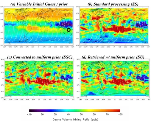
Figures 1 and 2 show the initial and retrieved values at 681 hPa for ozone and carbon monoxide, respectively, for datasets SS, SU, and SSC. The TES target locations are shown with white +’s and interpolation is done between the TES targets. The TES stan-dard prior for both figures (panel a) is taken from a climatological run of the MOZART-3 model binned by 60 degrees longitude, and 10 degrees latitude. For the ozone prior,

25

(8)

ACPD

8, 1261–1289, 2008

Full Screen / Esc

Printer-friendly Version Interactive Discussion and an enhanced band from South America through southern Africa to Australia (the

biomass burning region (discussed iiin Bowman et al., 2007)), and a minimum is seen north of Australia. The standard retrieval shown in Fig. 1b represents these same pat-terns with a marked enhancement in the biomass burning region. The constant prior cases (panels c and d) agree remarkably well with each other indicating that the linearly

5

converting the prior is valid throughout most of the data. The features in panels c and d can be confidently attributed to the TES data without preconceptions introduced by the prior; however large differences between panels b and c or d indicate a dependence on the prior rather than the data. The absence or presence of particular points passing quality flags can cause minor changes in the three different results. Most of ozone

10

enhancements between 60 S–60 N remain between the standard processing and the converted prior (Fig. 1b and c) indicating that TES retrievals are sensitive at this pres-sure level over those regions. Poleward of 60 N, enhancements seen in the prior and the standard retrieval are absent, indicating that TES retrievals are insensitive in those regions.

15

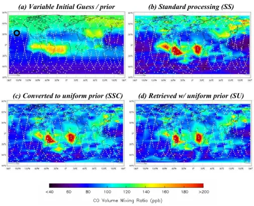
Figure 2 shows the same plots as in Fig. 1, for carbon monoxide. The carbon monox-ide prior (Fig. 2a) indicates enhancement over South America and southern Africa (in the biomass burning region), north of 40 N, and over India and southeast Asia. The standard retrieval Fig. 2b displays marked enhancement over the prior in eastern South America and western sub-Sahara Africa, and in eastern Asia. The uniform prior results,

20

panels c and d, show good agreement with each other. The East Asia enhancement is present but muted and the pattern and values in the biomass burning region are very similar between panels b, c, and d, however the CO enhancement poleward of 40 N is markedly reduced in c and d indicating that TES retrievals have less sensitivity in those regions.

25

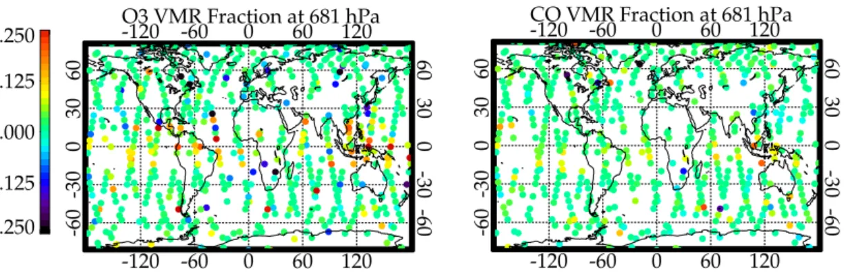
Figure 3 shows global maps of the VMR fractional difference (using Eq. 3) for O3and CO at 681 hPa for the SSC and SU datasets. The plots show that outliers occur pre-dominately in the tropics, and to a lesser extent, Antarctica. The pattern may suggest two cloud layers, which occur frequently in the tropics (Zipser, 1969), could contribute

(9)

ACPD

8, 1261–1289, 2008

Full Screen / Esc

EGU to the retrieval variation since TES assumes one cloud layer (Kulawik et al., 2006b),

however determining correlations between outliers and atmospheric conditions was not explored further in this paper.

3.1 Statistical analysis

To quantify differences, statistical analysis was done on the 681 targets which have

5

good quality flags for all three runs (SS (and by extension SSC), SU, and US). The quality flags check for retrieval convergence using thresholds for the radiance residual and mean, maximum allowed changes in the retrieved surface temperature or emissiv-ity, the amount of signal remaining in the residual; or other known issues (Osterman et al., 2007). The quality flags are set to screen out about 80% of the bad cases, but will

10

also screen out perhaps 20% of good cases as well (Osterman et al., 2007).

A histogram of the fractional difference between the SSC and SU datasets shows the overall accuracy of changing the prior using Eq. (2) vs. using a uniform prior in the non-linear retrieval. From this histogram several relevant quantities can be calculated: (1) the fraction of the targets are within 5% of each other, (2) the fractional difference

15

that encompasses 95% of the targets, and (3) the standard deviation of the fractional difference.

3.1.1 Results for ozone

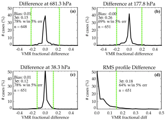
In Fig. 4, a histogram of the VMR fractional difference, using Eq. (3), is shown compar-ing dataset SSC (the standard retrieval converted to a uniform prior uscompar-ing Eq. (2) to SU

20

(the non-linear retrieval using a uniform prior) at 681, 178, 38 hPa, and over the entire profile. Figure 4 shows that for ozone, 70–80% of the SSC and SU results are within 5% difference. It is not surprising that histogram for the 177.8 hPa pressure level has the widest spread among the 3 pressure levels chosen because ozone at that pres-sure level has an order of magnitude variability due to the variations in the tropopause

25

(10)

ACPD

8, 1261–1289, 2008

Full Screen / Esc

Printer-friendly Version Interactive Discussion to the retrieval. Note that the errors introduced by changing the prior are small when

compared to the TES reported total error (green dashed line in Fig. 4). In comparison, the VMR fractional difference of the prior had a 1-sigma value of 0.41, 1.08 (i.e. 108%), and 0.16 at 681, 178, and 38 hPa, respectively, indicating significantly more spread in the prior than in the resulting retrieval. The 1-sigma values for the results are shown in

5

Table 1.

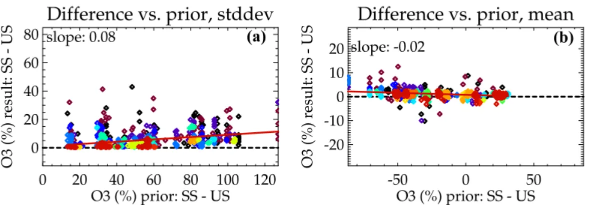
The histograms in Fig. 4 all show sharp peaks centered near zero but also show more outliers than would be expected from a Gaussian distribution. To determine if the outlying points are a result of a breakdown in the linear transform in Eq. (2) that occurs when the a priori change is too large, the difference (SSC-SU) is plotted versus

10

the change in the prior, averaged over the profile, in Fig. 5. Figure 5 shows no obvious difference between small and large prior changes. In Fig. 5, panel a shows the rms of (SSC-SU), and panel b shows the mean difference, both averaged over the entire profile. For the rms difference, the slope tells whether, on average, larger differences in the prior lead to larger differences in the results. This slope was 0.10. For the mean

15

difference, the slope indicates if the changes in the prior bias the results. The slope of this was found to be −0.02. Together these results mean that less than 10% of the prior’s change will end up as unbiased fluctuations in the answer. The lack of bias show that the differences are not a function of the choice of the uniform prior.

To check the whether the outliers in Fig. 4 are a result of converging to a different

20

local minimum, a run was done with a globally uniform initial guess (dataset US). The initial guess is the starting location for the retrieval, which iterates until convergence is reached. Since the initial guess is not included in the cost function, which determines the final solution, it should not affect the retrieval assuming the retrieval gets to the global minimum. However, an initial guess far from true can lead the retrieval to a

non-25

global minimum, and systematic errors in the forward model or observed radiance can roughen the error landscape and introduce local minima. A more complete description of TES retrievals is discussed in Bowman et al. (2006). Theoretically, the initial guess does not influence the results (as seen also in Eq. (1) and dataset US should

(11)

con-ACPD

8, 1261–1289, 2008

Full Screen / Esc

EGU verge to the same answer as the standard retrieval (dataset SS). Differences in these

datasets indicate convergence to different local minima, but we do not know whether either has reached a global minimum. The histograms from this run for ozone are shown in Fig. 6. In general, histograms of SS vs. US show a sharper peak and more outliers than the histograms from Fig. 4. For O3 at 681 hPa, for example, 17% of

tar-5

gets change greater than the TES reported error compared to 2% for results shown in Fig. 4.

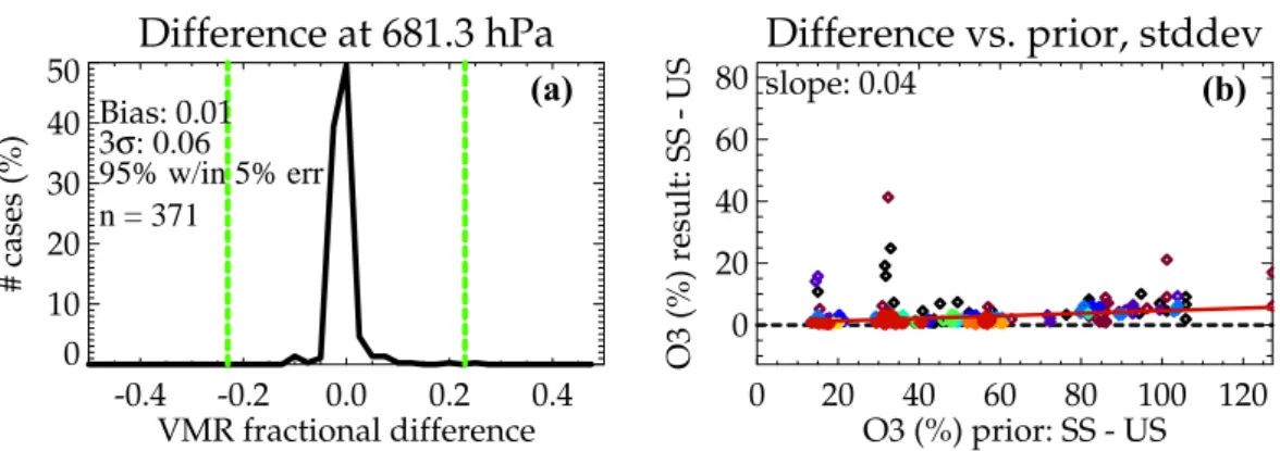
Figure 7 has all “initial guess outliers” removed, and compares remaining targets for datasets SSC and SU. “Initial guess outliers” are set to be those where the average rms difference over the profile between SS and US were more than 5%, and represent

10

targets that show a tendency to converge to different minima. Results are shown in Fig. 7 for 681 hPa, and correlations shown for the profile standard deviation. In this case, there are significantly fewer outliers (compared to Figs. 4 and 5). The right plot in Fig. 7 shows that the spread in the prior is still about the same, but that the spread in the result is markedly less. This means that the outliers in Figs. 4 and 5 likely result

15

from retrievals converging to different local minima. Table 1 summarizes the results for Figs. 4, 5, and 7 for ozone.

As discussed following Eq. (2), when a retrieval is not sensitive, it will converge to the prior and exchanging the prior will move the retrieval to the new prior, as seen for retrievals poleward of 60 N in Fig. 1. The effects of changing the prior on the most

20

sensitive points is of interest, so statistics were calculated for only those points with a corresponding averaging kernel diagonal value of 0.04 or greater. For 681 hPa, the number of samples dropped from 648 to 290; the bias increased from 0.01 to 0.02, the 1-sigma value increased from 2.0% to 2.7%, the 3-sigma value increased from 15% to 17%, and the fraction within 5% error dropped from 78% to 65%. For 177.8 hPa and

25

38.3 hPa, the changes are smaller, for example for 38.3 hPa the fraction within 5% error dropped from 78% to 72%. However the result that the error is unbiased and smaller than the reported total error still holds true for the most sensitive points.

(12)

ACPD

8, 1261–1289, 2008

Full Screen / Esc

Printer-friendly Version Interactive Discussion 3.1.2 Results for carbon monoxide

For TES retrievals, carbon monoxide is retrieved following the retrieval of tempera-ture/water/ozone steps. Consequently, changes to the temperature, surface temper-ature, or cloud parameters resulting from the uniform ozone prior will propagate into differences in the carbon monoxide step. Swapping only the carbon monoxide, rather

5

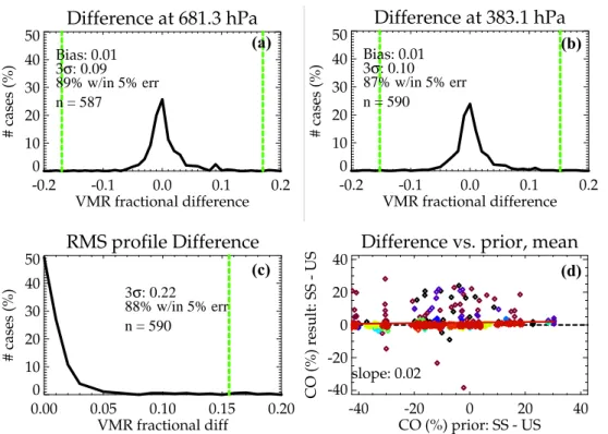
than all the species together, may improve on the results shown in this study. Fig-ure 8 shows the histogram of the fractional VMR change for CO at 383 and 681 hPa (note Figs. 8 and 9 do not have initial guess outliers removed). Additionally results are shown for averages over the entire profile. Carbon monoxide shows fewer outliers beyond 10% than found with ozone. Results for CO are summarized in Table 2. In

10

comparison, the VMR fractional difference of the prior had a 1-sigma value of 0.30 and 0.17 at 681 and 381 hPa, respectively, indicating significantly more spread in the prior change than in the resulting retrieval.

3.1.3 Results for methane

Methane is also retrieved following the temperature/water/ozone steps, and changes to

15

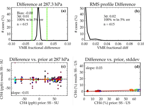
the temperature, surface temperature, or cloud parameters resulting from the uniform ozone prior will propagate into differences in the methane step. The results seen in this study are likely to be worse than the results from swapping only the methane. Figure 9 shows results at 287 hPa and for the whole profile, and shows that changing to a uniform prior results in less than a 1% difference in methane for 95% of the cases.

20

Results for methane are summarized in Table 3. In comparison, the VMR fractional difference of the prior had a 1-sigma value of 0.06 at 287 hPa indicating significantly more spread in the prior change than in the resulting retrieval.

(13)

ACPD

8, 1261–1289, 2008

Full Screen / Esc

EGU 3.1.4 Error analysis differences when changing the prior

When one changes to a different prior following the nonlinear retrieval, the error anal-ysis available is the one calculated at the original retrieval. This section determines whether this error analysis is accurate by looking the change in the averaging kernel between runs SS and SU. We compare the total degrees of freedom for signal, and at

5

individual values in the averaging kernel diagonal, through comparisons of the mean values, and at the fractional difference (calculated for values greater than 0.001).

For ozone, the mean degrees of freedom for signal (DOF) is 3.80. The mean DOF changes 0.01 between the two runs. The rms difference of the DOF is 0.04, which is about 1%. The mean value of the averaging kernel diagonal between the surface and

10

10 hPa is 0.069. The mean difference between the two runs is 8×10−5, and the rms fractional difference of the averaging kernel diagonals are 15%.

For retrievals in Log(VMR), sensitivity is positively correlated to the VMR (Deeter et al., 2007). We find that retrievals with a 10% increase in the retrieved ozone column density also have about a 0.15 increase in the degrees of freedom, a 4% increase.

15

Since the uniform prior is set to the global mean, this does not cause a biased change between the two runs for this test.

For carbon monoxide, the mean DOF is 1.09, with a mean difference of 0.004 be-tween the two runs. The rms difference is 0.02, or 2%. The mean value of the aver-aging kernel diagonal between the suface and 10 hPa is 0.039. The mean difference

20

between the two runs is 0.0006, and the rms fractional difference of the averaging kernel diagonals are 22%.

For methane, the mean DOF is 1.27, with a mean difference of 8×10−6between the two runs. The rms difference is 0.04, or 3%. The mean value of the averaging kernel diagonal between the suface and 10 hPa is 0.024. The mean difference between the

25

two runs is 0.00003, and the rms fractional difference of the averaging kernel diagonals are 12%.

(14)

ACPD

8, 1261–1289, 2008

Full Screen / Esc

Printer-friendly Version Interactive Discussion and the individual averaging kernel diagonal values vary by about 20%. This indicates

that the error bars and sensitivities may have about a 20% unbiased change for any particular level when the prior is changed, however the total DOF remains fairly imper-vious to changes in the prior.

4 Conclusions

5

Linearly converting the prior following a non-linear retrieval is shown to have a minor ef-fect on TES trace gas retrievals as compared to a non-linear retrieval using the desired prior, when compared to the reported total error. Histograms of differences between these two methods show a sharp peak centered near zero with some outliers, espe-cially for ozone. Further analysis of the characteristics of the outliers, and comparisons

10

to retrievals with a uniform initial guess indicates that the many of the outliers result from convergence to a local minimum rather than breakdown of the linear conversion in Eq. (2). For ozone, the 1-sigma difference is less than 4% for each of three pressure levels studied, and the mean change for all levels is 2.7%. For methane, the 1-sigma change is 0.3% at 287 hPa and 0.3% for the profile average, and for carbon monoxide

15

the 1-sigma change is about 2%. The degrees of freedom comparison between shows a 1-sigma difference of less than 3% for all the species, and shows changes of the averaging kernel diagonal are on the order of 20% for individual levels.

(15)

ACPD

8, 1261–1289, 2008

Full Screen / Esc

EGU

Acknowledgements. Thanks to members of the TES science team and the TES software team.

This work was performed at the Jet Propulsion Laboratory, California Institute of Technology, under a contract with the National Aeronautics and Space Administration.

References

Beer, R.: TES on the Aura mission: Scientific objectives, measurements, and analysis

5

overview, IEEE T. Geosci. Remote, 44, 5, 1102–1105, 2006.

Bowman, K. W., Worden, J., Steck, T., Worden, H. M., Clough, S., and Rodgers, C.: Capturing time and vertical variability of tropospheric ozone: A study using TES nadir retrievals, J. Geophys. Res.-Atmos., 107(D23), 4723, doi:10.1029/2002JD002150, 2002.

Bowman, K. W., Rodgers, C. D., Kulawik, S. S., Worden, J., Sarkissian, E., Osterman, G.,

10

Steck, T., Lou, M., Eldering, A., Shephard, M., Worden, H., Lampel, M., Clough, S., Brown, P., Rinsland, C., Gunson, M., and Beer, R.: Tropospheric emission spectrometer: Retrieval method and error analysis, IEEE T. Geosci. Remote, 44, 5, 1297–1307, 2006.

Bowman, K. W., Jones, D. B. A., Logan, J. A., Worden, H. M., Boersma, F., Kulawik, S. S., Osterman, G., Worden, J. R., and Chang, R.: Impact of surface emissions to the zonal

15

variability of tropical tropospheric ozone and carbon monoxide for November 2004, Atmos. Chem. Phys. Discuss., accepted, 2007.

Brasseur, G. P., Hauglustaine, D. A., Walters, S., Rasch, P. J., Muller, J. F., Granier, C., and Tie, X. X.: MOZART, a global chemical transport model for ozone and related chemical tracers 1. Model description, J. Geophys. Res.-Atmos., 103(D21), 28 265–28 289, 1998.

20

Deeter, M. N., Emmons, L. K., Francis, G. L., Edwards, D. P., Gille,J. C., Warner,J. X., Khat-tatov, B., Ziskin, D., Lamarque, J. F., Ho, S. P., Yudin, V., Attie, J. L., Packman, D., Chen, J., Mao, D., and Drummond, J. R.: Operational carbon monoxide retrieval algorithm and selected results for the MOPITT instrument, J. Geophys. Res.-Atmos., 108(D14), 4399, doi:10.1029/2002JD003186, 2003.

25

Deeter, M. N., Edwards, D. P., and Gille, J. C.: Retrievals of carbon monoxide profiles from MO-PITT observations using lognormal a priori statistics, J. Geophys. Res.-Atmos., 112(D11), D11311, doi:10.1029/2006JD007999, 2007.

Kulawik, S. S., Worden, H., Osterman, G., Luo, M., Beer, R., Kinnison, D. E., Bowman, K. W., Worden, J., Eldering, A., Lampel, M., Steck, T., and Rodgers, C. D.: TES atmospheric profile

(16)

ACPD

8, 1261–1289, 2008

Full Screen / Esc

retrieval characterization: An orbit of simulated observations, IEEE T. Geosci. Remote, 44, 5, 1324–1333, 2006a.

Jones, D. B. A., Bowman, K. W., Palmer, P. I., Worden, J. R., Jacob, D. J., Hoffman, R. N., Bey, I., and Yantosca, R. M.: Potential of observations from the Tropospheric Emission Spectrometer to constrain continental sources of carbon monoxide, J. Geophys. Res.-Atmos., 108(24),

5

4789, doi:10.1029/2003JD003702, 2003.

Kulawik, S. S., Worden, J., Eldering, A., Bowman, K., Gunson, M., Osterman, G. B., Zhang, L., Clough, S. A., Shephard, M. W., and Beer, R.: Implementation of cloud retrievals for Tropo-spheric Emission Spectrometer (TES) atmoTropo-spheric retrievals: part 1: Description and char-acterization of errors on trace gas retrievals, J. Geophys. Res.-Atmos., 111(D24), D24204,

10

doi:10.1029/2005JD006733, 2006b.

Logan, J. A., Megretskaia, I., Nassar, R., Murray, L. T., Zhang, L., Bowman, K. W., Helen Worden, H. M., and Luo, M.: The effects of the 2006 El Ni ˜no on tropospheric composition as revealed by data from the Tropospheric Emission Spectrometer (TES), Geophys. Res. Lett., accepted, 2007.

15

Luo M., Rinsland, C. P., Rodgers, C. D., Logan, J. A., Worden, H., Kulawik, S., Eldering, A., Goldman, A., Shephard, M. W., Gunson, M., and Lampel, M.,: Comparison of carbon monoxide measurements by TES and MOPITT: the influence of a priori data and instrument characteristics on nadir atmospheric species retrievals, J. Geophys. Res., 112, D09303, doi:101029/2006JD007663, 2007.

20

Luo, M., Rinsland, C., Fisher, B., Sachse, G., Diskin, G., Logan, J., Worden, H., Kulawik, S., Osterman, G., Eldering, A., Herman, R., and Shephard, M.,: TES carbon monoxide validation with DACOM aircraft measurements during INTEX-B 2006, J. Geophys. Res., in press, 2007.

Nassar, R., Logan, J. A., Worden, H. M., Megretskaia, I. A. Bowman, K. W., Osterman, G.

25

B., Thompson A. M., Tarasick, D. W., Austin, S., Claude, H., Dubey, M. K., Hocking, W. K., Johnson, B. J., Joseph, E., Merrill, J., Morris, G. A., Newchurch, M., Oltmans, S. J., Posny, F., Richards, F. J. N. A. D., et al.: Validation of Tropospheric Emission Spectrom-eter (TES) Ozone Profiles with Aircraft Observations During INTEX-B, J. Geophys. Res., accepted, 2007.

30

Osterman, G., Bowman, K. R., Eldering, A., Fisher, B., Herman, R., Jacob, D., Jourdain, L., Ku-lawik, S. S., Luo, M., Monarrez, R., Paradise, S., Poosti, S., Richards, N., Rider, D., Shepard, D., Vilnrotter, F., Worden, H., Worden, J., and Yun, H.: Tropospheric Emission Spectrometer

(17)

ACPD

8, 1261–1289, 2008

Full Screen / Esc

EGU TES L2 Data User’s Guide (Up to & including Version F04 04 data), Jet Propulsion

Labora-tory, California Institute of Technology, Pasadena, CA, 508, 2006.

Park, M., Randel, W. J., Kinnison, D. E., Garcia, R. R., and Choi, W.: Seasonal variation of methane, water vapor, and nitrogen oxides near the tropopause: Satel-lite observations and model simulations, J. Geophys. Res.-Atmos., 109(D3), D03302,

5

doi:10.1029/2003JD003706, 2004.

Rienecker, M. M., Suarez, M. J., Todling, R., Bacmeister, J., Takacs, L., Liu, H.-C., Gu, W., Sienkiewicz, M., Koster, R. D., Gelaro, R., and Stajner, I.: The GEOS-5 Data Assimila-tion System: A DocumentaAssimila-tion of GEOS-5.0/NASA TM 104606, Technical Report Series on Global Modeling and Data Assimilation, *v27*, 2006.

10

Rinsland, C. P., Luo, M., Logan, J. A., Beer, R., Worden, H., Kulawik, S. S., Rider, D., Oster-man, G., Gunson, M., Eldering, A., GoldOster-man, A., Shephard, M., Clough, S. A., Rodgers, C., Lampel, M., and Chiou, L.: Nadir measurements of carbon monoxide distributions by the Tropospheric Emission Spectrometer instrument onboard the Aura Spacecraft: Overview of analysis approach and examples of initial results, Geophys. Res. Lett., 33(22), L22806,

15

doi:10.1029/2006GL027000, 2006.

Rodgers, C.: Inverse Methods for Atmospheric Sounding: Theory and Practice, World Scientific Publishing Co., Singapore, 2000.

Rodgers, C. D. and Connor B. J.: Intercomparison of remote sounding instruments, J. Geophys. Res.-Atmos., 108(D3), 4116, doi:10.1029/2002JD002299, 2003.

20

Shephard, M. W., Herman, R. L., Fisher, B. M., Cady-Pereira, K. E., Clough, S. A., Payne, V. H., Whiteman, D. N., Comer, J. P., V ¨omel, H., Milosevich, L. M., Forno, R., Adam, M., Osterman, G. B., Eldering, A., Worden, J. R., Brown, L. R., Worden, H. M., Kulawik, S. S., Rider, D. M., Goldman, A., Beer, R., Bowman, K. W., Rodgers, C. D., Luo, M., Rinsland, C. P., Lampel, M., and Gunson, M. R.: Comparison of Tropospheric Emission Spectrometer (TES) Water

25

Vapor Retrievals with In Situ Measurements, J. Geophys. Res., accepted, 2007.

Worden, H. M., Logan, J., Worden, J. R., Beer, R., Bowman, K., Clough, S. A., Eldering, A., Fisher, B., Gunson, M. R., Herman, R. L., Kulawik, S. S., Lampel, M. C., Luo, M., Megret-skaia, I. A., Osterman, G. B., and Shephard, M. W.: Comparisons of Tropospheric Emission Spectrometer (TES) ozone profiles to ozonesodes: methods and initial results, J. Geophys.

30

Res., 112, D03309, doi:10.1029/2006JD007258, 2007.

Worden, H. M., Logan, J. A., Worden, J. R., Beer, R., Bowman, K., Clough, S. A., Eldering, A., Fisher, B. M., Gunson, M. R., Herman, R. L., Kulawik, S. S., Lampel, M. C., Luo, M.,

(18)

ACPD

8, 1261–1289, 2008

Full Screen / Esc

Megretskaia, I. A., Osterman, G. B., and Shephard, M. W.: Comparisons of Tropospheric Emission Spectrometer (TES) ozone profiles to ozonesondes: Methods and initial results, J. Geophys. Res.-Atmos., 112(D3), D03309, doi:10.1029/2006JD007258, 2007.

Worden, J., Noone, D., and Bowman, K.: Importance of rain evaporation and continental con-vection in the tropical water cycle, Nature, 445, 7127, 528–532, 2007.

5

Zhang, L., Jacob, D. J., Bowman, K. W., Logan, J. A., Turquety, S., Hudman, R. C., Li, Q. B., Beer, R., Worden, H. M., Worden, J. R., Rinsland, C. P., Kulawik, S. S., Lampel, M. C., Shephard, M. W., Fisher, B. M., Eldering, A., and Avery, M. A.: Ozone-CO correlations determined by the TES satellite instrument in continental outflow regions, Geophys. Res. Lett., 33(18), L18804, doi:10.1029/2006GL026399, 2006.

10

Zipser, E. J.: The role of organized unsaturated convective downdrafts in the structure and rapid decay of an equatorial disturbance, J. Appl. Meteorol., 8, 799–814, 1969.

(19)

ACPD

8, 1261–1289, 2008

Full Screen / Esc

EGU Table 1. Summary of the differences between the linear vs. non-linear application of a uniform

prior for ozone.

1a – all good quality cases

Quantity 681 hPa 178 hPa 38 hPa Average 1-sigma % difference 2.0% 3.8% 1.3% 2.7% w/in 5% difference 78% 69% 78% 64% 95% w/in range _±0.15 _±0.26 _±0.12 _±0.18 Slope (see Fig. 5) _−0.04 0.00 _−0.07 _−0.02*

1b – screened by convergence which is indicated by the initial guess results Quantity 681 hPa 178 hPa 38 hPa Average 1-sigma % difference 1.1% 1.6% 1.0% 0.7%

w/in 5% difference 95% 88% 94% 90%

95% w/in range _±0.06 _±0.12 _±0.05 _±0.06

slope 0.01 0.01 _−0.02 _−0.01*

* The slope is calculated for the mean difference of the profiles. The other average quantities are calculated for the rms difference.

(20)

ACPD

8, 1261–1289, 2008

Full Screen / Esc

Printer-friendly Version Interactive Discussion Table 2. Summary of the differences between the linear vs. non-linear application of a uniform

prior for carbon monoxide.

Quantity 681 hPa 383 hPa Average*

1-sigma 0.8% 2.0% 1.1%

w/in 5% difference 89% 87% 88% 95% w/in range _±0.09 _±0.10 _±0.22

Slope 0.02 0.07 0.02

(21)

ACPD

8, 1261–1289, 2008

Full Screen / Esc

EGU Table 3. Table 3. Summary of the differences between the linear vs. non-linear application of

a uniform prior for methane

Quantity 287 hPa Average*

1-sigma 0.3% 0.3%

w/in 5% difference 100% 100% 95% w/in range _±0.01 _±0.02

slope _−0.01 _−0.01

(22)

ACPD

8, 1261–1289, 2008

Full Screen / Esc

(a) Variable Initial Guess / prior (b) Standard processing (SS)

(c) Converted to uniform prior (SSC) (d) Retrieved w/ uniform prior (SU)

Fig. 1. TES retrieved ozone at 681 hPa. Panel (a) shows the standard globally variable TES

a priori and initial states, with observation location shown with white +’s. Panel (b) shows the TES standard retrieval (SS). Panel (c) shows the TES standard retrieval converted to a uniform prior (SSC). Panel (d) shows TES retrieved with a uniform prior (SU). Panels (c) and (d) should agree in the linear regime. The circle in panel (a) shows the value of the uniform prior at this pressure which is 48 ppb. The color scale, which is the same for all plots, is shown below all 4 plots.

(23)

ACPD

8, 1261–1289, 2008

Full Screen / Esc

EGU

(a) Variable Initial Guess / prior (b) Standard processing (SS)

(c) Converted to uniform prior (SSC) (d) Retrieved w/ uniform prior (SU)

Fig. 2. TES retrieved carbon monoxide at 681 hPa. Panel (a) shows the variable TES a priori. Panel (b) shows the TES standard retrieval (SS). Panel (c) shows the TES standard retrieval converted to a uniform prior (SSC). Panel (d) shows TES retrieved with a uniform prior (SU). Panels (c) and (d) should agree in the linear regime. The circle in panel (a) shows the approximate value of the uniform prior at this pressure (97 ppb).

(24)

ACPD

8, 1261–1289, 2008

Full Screen / Esc

Printer-friendly Version Interactive Discussion -120 -60 0 60 120 -120 -60 0 60 120 -60 -30 0 30 60 -60 -30 0 30 60 O3 VMR Fraction at 681 hPa -0.250 -0.125 0.000 0.125 0.250 -120 -60 0 60 120 -120 -60 0 60 120 -60 -30 0 30 60 -60 -30 0 30 60 CO VMR Fraction at 681 hPa

Fig. 3. VMR fraction difference for SSC-SU for O3(left) and CO (right) at 681 hPa. These plots show that the outliers occur predominately in the tropics.

(25)

ACPD

8, 1261–1289, 2008

Full Screen / Esc

Printer-friendly Version Interactive Discussion EGU Difference at 681.3 hPa -0.4 -0.2 0.0 0.2 0.4 VMR fractional difference 0 10 20 30 40 50 # cases (%) Bias: 0.01 3σ: 0.15 78% w/in 5% err n = 648 Difference at 177.8 hPa -0.4 -0.2 0.0 0.2 0.4 VMR fractional difference 0 10 20 30 40 50 # cases (%) Bias: -0.00 3σ: 0.26 69% w/in 5% err n = 651 Difference at 38.3 hPa -0.4 -0.2 0.0 0.2 0.4 VMR fractional difference 0 10 20 30 40 50 # cases (%) Bias: 0.01 3σ: 0.12 78% w/in 5% err n = 651 RMS profile Difference 0.0 0.1 0.2 0.3 0.4 0.5 VMR fractional diff 0 10 20 30 40 50 # cases (%) 3σ: 0.18 64% w/in 5% err n = 651 (c) (d) (a) (b)

Fig. 4. Statistical comparison between non-linear retrievals using a uniform prior (SU) vs.

conversion to a uniform prior using Eq. (2) (SSC). The black line shows the histogram of the Fractional difference of (SSC-SU) for 3 different pressure levels. The green dashed line is the mean TES reported total error. The lower right plot is the standard deviation of the VMR fractional difference averaged over the entire profile.

(26)

ACPD

8, 1261–1289, 2008

Full Screen / Esc

Difference vs. prior, stddev

0 20 40 60 80 100 120 O3 (%) prior: SS - US 0 20 40 60 80 O3 (%) result: SS - US slope: 0.08

Difference vs. prior, mean

-50 0 50 O3 (%) prior: SS - US -20 -10 0 10 20 O3 (%) result: SS - US slope: -0.02 (a) (b)

Fig. 5. Change in (SSC-SU) as a function of the change in the prior. The colors represent

density of points using the same color progression as used in Figs. 1 and 2, where red indicates the highest density of points. The calculated slope is shown as a red line. These results indicate that less than 10% of the prior’s change will end up as unbiased fluctuations in the answer.

(27)

ACPD

8, 1261–1289, 2008

Full Screen / Esc

Printer-friendly Version Interactive Discussion EGU

Difference at 681.3 hPa

-0.4 -0.2 0.0 0.2 0.4 VMR fractional difference 0 10 20 30 40 50 # cases (%) Bias: 0.05 3σ: 0.81 67% w/in 5% err n = 648

Difference at 177.8 hPa

-0.4 -0.2 0.0 0.2 0.4 VMR fractional difference 0 10 20 30 40 50 # cases (%) Bias: -0.12 3σ: 0.87 62% w/in 5% err n = 651 (a) (b)

Fig. 6. Statistical comparison between non-linear retrievals using a globally constant initial

guess vs. variable initial gues. The black line shows the histogram of the VMR fractional difference for SS-US for 2 different pressure levels (681 and 178 hPa).

(28)

ACPD

8, 1261–1289, 2008

Full Screen / Esc

Difference at 681.3 hPa

-0.4 -0.2 0.0 0.2 0.4 VMR fractional difference 0 10 20 30 40 50 # cases (%) Bias: 0.01 3σ: 0.06 95% w/in 5% err n = 371

Difference vs. prior, stddev

0 20 40 60 80 100 120 O3 (%) prior: SS - US 0 20 40 60 80 O3 (%) result: SS - US slope: 0.04 (a) (b)

Fig. 7. The effects of removing outliers on the prior comparison. Cases which are outliers from

swapping the initial guess are removed from the prior comparison. The remaining cases show better characteristics compared to Figs. 4 and 5.

(29)

ACPD

8, 1261–1289, 2008

Full Screen / Esc

Printer-friendly Version Interactive Discussion EGU Difference at 681.3 hPa -0.2 -0.1 0.0 0.1 0.2 VMR fractional difference 0 10 20 30 40 50 # cases (%) Bias: 0.01 3σ: 0.09 89% w/in 5% err n = 587 Difference at 383.1 hPa -0.2 -0.1 0.0 0.1 0.2 VMR fractional difference 0 10 20 30 40 50 # cases (%) Bias: 0.01 3σ: 0.10 87% w/in 5% err n = 590 RMS profile Difference 0.00 0.05 0.10 0.15 0.20 VMR fractional diff 0 10 20 30 40 50 # cases (%) 3σ: 0.22 88% w/in 5% err n = 590

Difference vs. prior, mean

-40 -20 0 20 40 CO (%) prior: SS - US -40 -20 0 20 40 CO (%) result: SS - US slope: 0.02 (c) (d) (a) (b)

Fig. 8. Statistical comparison for carbon monoxide between non-linear retrievals using a

uni-form prior vs. conversion to a uniuni-form prior using Eq. (2). The black line shows the histogram of the VMR fractional difference of SSC and SU using Eq. (3) for 2 different pressure levels for carbon monoxide. The lower right panel shows the mean change in the result vs. the mean change in the prior.

(30)

ACPD

8, 1261–1289, 2008

Full Screen / Esc

Printer-friendly Version Interactive Discussion Difference at 287.3 hPa -0.10 -0.05 0.00 0.05 0.10 VMR fractional difference 0 10 20 30 40 50 # cases (%) Bias: -0.00 3σ: 0.01 100% w/in 5% err n = 615 RMS profile Difference 0.00 0.02 0.04 0.06 0.08 0.10 VMR fractional diff 0 10 20 30 40 50 # cases (%) 3σ: 0.02 100% w/in 5% err n = 615

Difference vs. prior at 287 hPa

-50 0 50 CH4 (ppb) prior: SS - SU -50 0 50 CH4 (ppb) result: SS - SU slope: -0.01

Difference vs. prior, stddev

0 10 20 30 40 50 60 CH4 (%) prior: SS - US 0 10 20 30 40 CH4 (%) result: SS - US slope: 0.03 (c) (d) (a) (b)

Fig. 9. Statistical comparison for methane between non-linear retrievals using a uniform prior

vs. conversion to a uniform prior using Eq. (2). The black line shows the histogram of the Fractional difference using Eq. (3) of SSC-SU for 287 hPa. The red line shows the histogram of the differences in the priors, which show significantly more spread. The upper right panel shows the histogram of the average error for all pressures. The lower right panel shows the difference in the retrieval result vs. the difference in the prior for 287 hPa, and the lower right is the same for the mean difference over the whole profile.