HAL Id: tel-01430044
https://tel.archives-ouvertes.fr/tel-01430044
Submitted on 9 Jan 2017HAL is a multi-disciplinary open access archive for the deposit and dissemination of sci-entific research documents, whether they are pub-lished or not. The documents may come from teaching and research institutions in France or abroad, or from public or private research centers.
L’archive ouverte pluridisciplinaire HAL, est destinée au dépôt et à la diffusion de documents scientifiques de niveau recherche, publiés ou non, émanant des établissements d’enseignement et de recherche français ou étrangers, des laboratoires publics ou privés.
aircraft structures
Liu Chu
To cite this version:
Liu Chu. Reliability and optimization, application to safety of aircraft structures. Mechanics [physics.med-ph]. INSA de Rouen, 2016. English. �NNT : 2016ISAM0008�. �tel-01430044�
THESE
Pour obtenir le diplôme de doctorat
Mécanique
Préparée au sein de INSA Rouen
Reliability and optimization, application to safety of
the aircraft structures
Présentée et soutenue par
Liu CHU
Thèse dirigée par José Eduardo SOUZA DE CURSI, Addelkhalak EL HAMI , laboratoire LOFIMS
Thèse soutenue publiquement le 24 Mars 2016 devant le jury composé de
M. P.BREITKOPF Directeur de recherche CNRS Rapporteur
M. X.L. GONG Professeur à l’U.T de Troyes Rapporteur
M. A. CHEROUAT
Professeur à l’U.T de Troyes Examinateur
M. M. EID PhD Ingénieur-Chercheur, au CEA, Paris Encadrant
M. A. EL HAMI Professeur à l’INSA de Rouen Directeur de thèse
I
In three years of Ph.D study, many people give me help and support in
the research work. Firstly, I would like to express my sincere gratitude to
my supervisor Prof. Eduardo Souza de Cursi, his guidance always keeps
me in the right way of study, constructive ideas from him in the process
of discussion inspire me a lot and are also very helpful in the work. His
deep mathematical foundation and extraordinary experiences in research
teach me how to be an excellent researcher.
Secondly, Prof. El Hami, as co-director of my thesis, also provides lots of
significant help. His passion in professional research encourages me to
have progress in the difficult questions. In addition, I also want to
appreciate M.M.Eid for his time and patience in the discussion.
Thirdly, thanks to my colleagues in the laboratory of LOFIMS
(Laboratoire d’Optimisation et FIabilité en Mécanique des Structures) for
their kindness and accompany in every day. The time spent with them is
a cherish memory for myself no matter where I will stay or who I will work
with in the future.
At last, I appreciate the organization of China Scholarship Council, the
scholarship from my country covers the expense of three years. My
family always stand by my side, it makes me have the courage to face
and come over the difficulty. Even though they never require my
appreciation or feedback, I want to present my best sincerely
acknowledgement to my family.
II
Tremendous struggles of researchers in the field of aerodynamic design and aircraft production were made to improve wing airfoil by optimization techniques. The development of computational fluid dynamic (CFD) in computer simulation cuts the expense of aerodynamic experiment while provides convincing results to simulate complicated situation of aircraft. In our work, we chose a special and important part of aircraft, namely, the structure of wing.
Reliability based optimization is one of the most appropriate methods for structural design under uncertainties. It struggles to seek for the best compromise between cost and safety while considering system uncertainties by incorporating reliability measures within the optimization. Despite the advantages of reliability based optimization, its application to practical engineering problem is still quite challenging. In our work, uncertainty analysis in numerical simulation is introduced and expressed by probability theory. Monte Carlo simulation as an effective method to propagate the uncertainties in the finite element model of structure is applied to simulate the complicate situations that may occur. To improve efficiency of Monte Carlo simulation in sampling process, Latin Hypercube sampling is performed. However, the huge database of sampling is difficult to provide explicit evaluation of reliability. Polynomial chaos expansion is presented and discussed. Kriging model as a surrogate model play an important role in the reliability analysis.
Traditional methods of optimization have disadvantages in unacceptable time-complexity or natural drawbacks of premature convergence because of finding the nearest local optima of low quality. Simulated Annealing is a local search-based heuristic, Genetic Algorithm draws inspiration from the principles and mechanisms of natural selection, that makes us capable of escaping from being trapped into a local optimum. In reliability based design optimization, these two methods were performed as the procedure of optimization. The loop of reliability analysis is running in surrogate model.
Key words: optimization, reliability, uncertainty analysis, heuristic method, Kriging model
III
Les chercheurs dans le domaine de la conception aérodynamique et de la fabrication des avions ont fait beaucoup d'effort pour améliorer les performances des ailes par des techniques d'optimisation. Le développement de la mécanique des fluides numérique a permi de réduire les dépenses en soufflerie tout en fournissant des résultats convaincants pour simuler des situations compliquées des aéronefs. Dans cette thèse, il a été choisi une partie spéciale et importante de l'avion, à savoir, la structure de l'aile.
L'optimisation basée sur la fiabilité est une méthode plus appropriées pour les structures sous incertitudes. Il se bat pour obtenir le meilleur compromis entre le coût et la sécurité tout en tenant compte des incertitudes du système en intégrant des mesures de fiabilité au sein de l'optimisation. Malgré les avantages de l'optimisation de la fiabilité en fonction, son application à un problème d'ingénierie pratique est encore assez difficile.
Dans notre travail, l'analyse de l'incertitude dans la simulation numérique est introduite et exprimée par la théorie des probabilités. La simulation de Monte Carlo comme une méthode efficace pour propager les incertitudes dans le modèle d'éléments finis de la structure est ici appliquée pour simuler les situations compliquées qui peuvent se produire. Pour améliorer l'efficacité de la simulation Monte Carlo dans le processus d'échantillonnage, la méthode de l'Hypercube Latin est effectuée. Cependant, l'énorme base de données de l'échantillonnage rend difficile le fait de fournir une évaluation explicite de la fiabilité. L'expansion polynôme du chaos est présentée et discutée. Le modèle de Kriging comme un modèle de substitution jouet un rôle important dans l'analyse de la fiabilité.
Les méthodes traditionnelles d'optimisation ont des inconvénients à cause du temps de calcul trop long ou de tomber dans un minimum local causant une convergence prématurée. Le recuit simulé est une méthode heuristique basée sur une recherche locale, les Algorithmes Génétiques puisent leur inspiration dans les principes et les mécanismes de la sélection naturelle, qui nous rendent capables d'échapper aux pièges des optimums locaux. Dans l'optimisation de la conception de base de la fiabilité, ces deux méthodes ont été mise en place comme procédure d'optimisation. La boucle de l'analyse de fiabilité est testée sur le modèle de substitution.
Mots – clés : optimisation, fiabilité, analyse de l'incertitude, méthode heuristique,
Acknowledgement ... I Abstract ... II Résumé ... III
Chapter 1 Introduction ... 1
1.1 Introduction of background ... 1
1.2 Outline of the dissetation ... 2
Chapter 2 Uncertainty analysis ... 5
2.1 Uncertainty classification ... 5
2.2 Sources of uncertainty ... 8
2.3 Uncertainty representation and modeling ... 9
2.3.1 Probability theory ... 9 2.3.2 Evidence theory ... 11 2.3.3 Possibility theory ... 12 2.3.4 Interval analysis ... 13 2.3.5 Convex modeling ... 13 2.4 Model validation ... 13
2.4.1 Pearson correlation coefficient ... 15
2.4.2 Spearman correlation coefficient ... 15
2.4.3 Kendall correlation coefficient ... 17
2.5 Sensitivity analysis ... 19
2.6 Uncertainty propagation ... 21
2.6.1 Monte Carlo simulation ... 21
2.6.2 Taylor series approximation ... 23
2.6.3 Reliability analysis ... 24
2.6.4 Decomposition based uncertainty analysis ... 24
2.7 Conclusion... 25
Chapter 3 Monte Carlo Simulation ... 27
3.1 Mathematical formulation of Monte Carlo Integration... 27
3.1.1 Plain (crude) Monte Carlo Algorithm ... 28
3.1.2 Geometric Monte Carlo Algorithm ... 29
3.2 Advanced Monte Carlo Methods ... 30
3.2.3 Latin Hypercube Sampling approach ... 33
3.3 Random Interpolation Quadratures ... 34
3.4. Iterative Monte Carlo Methods for Linear Equations ... 36
3.4.1 Iterative Monte Carlo Algorithms ... 37
3.4.2 Convergence and mapping ... 40
3.5 Morkov Chain Monte Carlo methods for Eigen-value Problem... 40
3.5.1 Formulation of Eigen-value problem ... 41
3.5.2 Method for Choosing the Number of Iterations k ... 44
3.5.3 Method for choosing the number of chains ... 45
3.6 Examples ... 46
3.6.1 Importance sampling ... 46
3.6.2 Latin Hypercube sampling in Finite element model of structure ... 50
3.7 Conclusion... 56
Chapter 4 Stochastic Expansion for Probability analysis ... 57
4.1 Fundamental of PCE ... 57
4.2 Stochastic approximation ... 58
4.3 Hermite Polynomials and Gram-Charlier Series ... 60
4.4 Karhunen-Loeve (KL) Transform ... 63
4.5 KL Expansion to solve Eigen value problem ... 65
4.6 Spectral Stochastic Finite Element Method ... 67
4.6.1 Role of KL expansion in SSFEM ... 67
4.6.2 Role of PCE in SSFEM ... 69
4.7 Examples ... 71
4.7.1 Orthogonal polynomial ... 71
4.7.2 Gram-Charlier series ... 74
4.7.3 Surrogate model for reliability analysis ... 75
4.8 Conclusion... 87
Chapter 5 Reliability based design optimization ... 89
5.1 General remarks of RBDO ... 90
5.1.1 Single Objective Optimization Description ... 91
5.1.2 Multiple-Objective Optimization description ... 93
5.2 First –order reliability method ... 95
5.2.3 Hasofer Lind- Rackwitz Fiessler (HL-RF) Method ... 103
5.2.4 FORM with adaptive approximations ... 105
5.3 Second-order Reliability Method (SORM) ... 106
5.3.1 First- and Second-order Approximation of Limit-state Function ... 107
5.3.2 Breitung’s Formulation ... 111
5.3.3 Tvedt’s Formulation ... 112
5.3.4 SORM with adaptive approximations ... 113
5.4 Mathematical Formulation of RBDO ... 113
5.4.1 RIA based RBDO ... 115
5.4.2 PMA based RBDO ... 115
5.5 Robust design optimization ... 116
5.6 Reliability based optimization in surrogate model ... 117
5.7 Conclusion... 129
Chapter 6 Examples ... 130
6.1 Cumulative Damage Analysis of Wing Structure by Stochastic Simulation ... 130
6.1.1 Stochastic simulation in Finite Element Model ... 130
6.1.2 Fatigue Analysis ... 134
6.1.3 Probability density ... 136
6.1.4 Conclusion ... 140
6.2 Airfoil shape optimization by heurist algorithms in surrogated model ... 141
6.2 .1 Airfoil CFD model ... 141
6.2.2 Surrogate model ... 143
6.2.3 Optimization ... 150
6.2.4 Conclusion ... 156
Chapter 7 Conclusion ... 157
Chapter 8 Résumé de la thèse en français ... 159
8.1 Motivation et objectif ... 159
8.2 Organisation du mémoire ... 160
8.2.1 Chapitre 2: Analyse de l'incertitude ... 161
8.2.2 Chapitre 3: simulation de Monte Carlo ... 162
8.2.3 Chapitre 4: Expansion stochastique pour l'analyse de probabilité ... 168
8.2.4 Chapitre 5: Fiabilité et optimisation ... 176
List of figures ... 201 List of tables ... 203 Reference ... 204
1
Chapter 1 Introduction
1.1 Introduction of background
As result of impressive advances in computational capability of hardware and software in recent decades, computational methods are gradually replacing empirical methods[1]. In the process of design and analyze aircraft components, more time and energy are spent in applying computational tools instead of conducting physical experiments[2].
For wing design, the requirement of new tools capable of accurate predicting aerodynamic behavior is performed. Numerical simulation of computational fluid dynamics can be applied for early detection of unwanted effects regarding stability and control behavior[3]. In the same time, uncertainty is an inevitable issue in the field of research. Since aircrafts have complicated operation environment and sophisticated mechanical structural itself.
The uncertainties in the aircraft can cause system performance to change or fluctuate, or even contribute to severe deviation and result in unprecedented function fault and mission failure. The consideration of uncertainty in the stage of design process is necessary[ 4 ]. According to specific characteristics of uncertainty, it should be represented in the research and design process by reasonable approaches.
The traditional analysis of deterministic Finite Element Model ignores the fluctuation of parameters as uncertain variables in the real operation environment. Application of Monte Carlo Method to probabilistic structural analysis problems is comparatively recent[ 5 ]. It is a powerful mathematical tool for determining the approximate probability of a specific event that is the outcome of a series of stochastic processes. Monte Carlo methods are useful and reliable only when a huge amount of sampling was performed[6]. It means heavy calculation burden of repeating sampling and time-consuming process to deal with result databases for grasping the key information. In the one hand, the struggles for reducing calculation expense in Monte Carlo Simulation are considerable. Among them, Latin Hypercube Sampling is one of advanced methods due to its advantage of having memory and effectiveness in the repeating sampling simulation[7]. In the other hand, sensitivity analysis is a way to
2
predict the importance level of one variable to the final outcome. By creating a given set of scenarios, the analyst can determine how changes in one variable will impact the target variable.
After perform Monte Carlo simulation in finite element models of aircraft structure, the huge database for the following reseach is also a big challenge to resarchers. Stochastic expansion for probability analysis is a promising method to provide believeable evalution in the next reliability analysis in our work. It also plays an important role in reducing the heavy calculation burden of reliability based design optimization.
1.2 Outline of the dissetation
In chapter 2, methods of uncertainty analysis are presented. Firstly, the uncertainty classification and sources of uncertainty in the simulated-design are discussed.Then we demonstrated uncertainty representation and modeling as concluded in the literatures. After that, model validation and sensitivity analysis are also taken into consideration. In the last part of this chapter, mentods of uncertatiny propagation are showed and discussed.
Chapter 3 begins with the introduction of mathematical formulation of Monte Carlo Integration. Next, we present advanced Monte Carlo methods, as importance sampling and Latin Hypercube sampling. Then, random interpolation quadratures, iterative Monte Carlo methods for linear equations and Morkow Chain Monte Carlo methods for Eigen-value problem are also demonstated in this chapter. Lastly, we have a numerical example of importance sampling method. Monte Carlo simulation in fininte element model of wing structure in chapter 3 is performed as original work. In Chapter 4, stochastic expansion for probability analysis is discussed. The fundamental theory of polynomial chaos expansion is presented in the first part of this chapter. Next, Hermite pomynomial and Gram – Charlier series are expressed. Then Karhunen – Loeve transform as a very useful method in simulation is also presented. In this chapter, we also explain the spectral stochastic finite element method, role of Karhunen – Loeve expansion and role of polynomial chaos expansion in spectral stochastic finite element method are demonstrated. Based on these theories, we also have serveral examples of stochastic expansion for probability analysis.
3
Chapter 5 presents reliability based design optimization. At first, general remarks of RBDO is illustrated. Then, first order and second order reliability method are explained. Next, we demonstrate mathematical formulation of RBDO. Robust design optimization is also introduced in this chapter. In the last part, examples of numerical simulation are presented.
In Chapter 6, two complet examples are demonstrated. The first example is cumulatice damage analysis of wing structure by stochastic simulation. As one of the most essential components in the aircraft structure, wing often operates in very complicated environment. It causes difficulties in identifying the exact values for the parameters in the models to simulate the real situation. In this example, a deterministic finite element model is created, the corresponding parameters in the model are sampled by Monte Carlo Method in numerous times. The process of stochastic simulation provides a useful database for the following cumulative damage analysis. Gaussian, Rayleigh, and Weibull distribution are proposed and used to express the probability density function for maximum stress in the wing structure. The last expression of probability distribution for maximum stress in the wing structure is polynomial function. In this method, sensitivity analysis was performed to find the most important several input variables. The relationship between the input variables and output variables in the database of stochastic simulation is obtained by linear regression method in the form of polynomial function. All of these four expressions were applied and discussed in cumulative damage analysis for wing structure.
The second example is airfoil shape optimization by heurist algorithms in surrogated model. Many struggles of researchers and designers in the field of aerodynamic design and aircraft production were made to improve wing airfoil by optimization techniques. Despite the development of computational fluid dynamic (CFD) in computer simulation, airfoil shape optimization is still quite challenging. In this example, we propose an effective method to have airfoil shape optimization by heuristic algorithms in surrogate model. To create an appropriate surrogate model, Monte Carlo simulation was performed by repeating computational fluid dynamic calculation, and reliable information was captured from this black box and concluded as Kriging interpolators. In order to prevent the premature convergence in the process optimization, attempts in heuristic algorithms for optimization were made.
4
The results of genetic algorithm and simulated annealing algorithm were tested in
CFD to confirm the reliability of the method proposed in this paper. Chapter 7 presents a summary of this dissertation, conclusions concerning the
5
Chapter 2 Uncertainty analysis
In the process of structural design, uncertainties include prediction errors induced by design model assumption and simplification; performance uncertainty arising from material properties, manufacturing tolerance; and uncertainty of load conditions applied on the structure during operation [2]. These uncertainties can cause system performance to change or fluctuate, or even contribute to severe deviation and result in unanticipated or even unprecedented function fault and mission failure.
Uncertainty analysis is the premise of uncertainty-based design optimization. It includes adopting suitable taxonomy to comprehensively identify and classify uncertainty sources; utilizing appropriate mathematical tools to represent and model these uncertainties; and applying sensitivity analysis approaches to screen out uncertainties with minor effects on design so as to simplify the problems.
2.1 Uncertainty classification
In different research fields, there are different definitions and taxonomies for the term of uncertainty. In computational modeling and simulation process, uncertainty is regarded as a potential deficiency in phases or activities of the modeling process caused by lack of knowledge[2] .
In some literatures, uncertainty is defined as the incompleteness in knowledge, and causes model-based predictions to differ from reality in a manner described by some distribution function[8] . In another useful functional definition it is defined as the information/knowledge gap between what is known and what needs to be known for optimal decisions with minimal risks[9].
From the perspective of systems engineering and taking the whole lifecycle into account during the design phase, the definition of uncertainty is as follows:
• Uncertainty: the incompleteness in knowledge and the inherent variability of the system and its environment.
• A robust system is defined to be relatively insensitive to variations in both the system components and the environment. The degree of tolerance to these variations is measured with robustness [4].
6
function without failure for a specified period of time under stated operating conditions[10].
To address uncertainty classification, the most popular uncertainty taxonomy is in risk assessment, which classifies uncertainty into two general categories: aleatory and epistemic.
• Aleatory uncertainty describes the inherent variation associated with the physical system or the environment under consideration. Sources of aleatory uncertainty can commonly be singled out from other contributors to nondeterministic simulation. Because their representation as distributed quantities can take on values in an established or known range, but the exact value will vary by chance from unit to unit or from time to time[11]. Aleatory uncertainty is also referred to in the literature as stochastic uncertainty, variability, inherent uncertainty, and cannot be eliminated by collection of more information or data.
• Epistemic uncertainty is due to lack of knowledge, and exists as a potential inaccuracy in any phase or activity of the modeling process. The first feature that our definition stresses is “potential”, in other words, the deficiency may or may not exist. It is possible that there is no deficiency even though lack of knowledge when model the phenomena correctly. The second key feature is that its fundamental cause is incomplete information due to vagueness, non-specificity, or dissonance. Epistemic uncertainty is known as subjective or cognitive, also referred to as reducible uncertainty and ignorance [6].
This taxonomy is widely accepted and has been applied in numerous fields. The conclusion of the difference between aleatoty uncertainty and epistemic uncertainty is clearly showed in Fig 2-1.
7
Fig 2 - 1 Comparison between aleatory uncertainty and epistemic uncertainty Besides aleatory and epistemic uncertainty, errors exist as a recognizable deficiency in phases of modeling and simulation. An error can be either acknowledged or unacknowledged.
Acknowledged errors[12] are deficiencies recognized or introduced by the analysts. Examples of acknowledged errors are finite precision arithmetic in a digital computer, approximations made to simplify the modeling of a physical process, and conversion of partial differential equations into discrete equations, or lack of spatial convergence. Acknowledged errors can be estimated, bounded, or ordered.
Examples of unacknowledged errors are blunders or mistakes. They can be programming errors, input or output errors, and compilation and linkage errors. There are no straightforward methods for estimating, bounding, or ordering the contribution of unacknowledged errors.
8
2.2 Sources of uncertainty
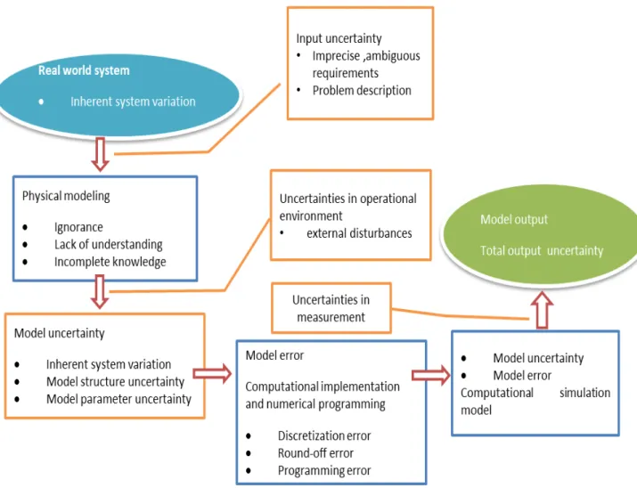
In the process of simulation-based design, uncertainties origins from four sources: input, operational environment, model uncertainties, and measurement; as showed in Fig 2-2 ,
• Input uncertainties are caused by imprecise or even ambiguous requirements and problems description.
• Uncertainties in operational environment are due to unknown or uncontrollable external disturbances.
• Model uncertainties include model structure uncertainty and model parameter uncertainty. Model structure uncertainty, also mentioned as non-parametric uncertainty, is mainly due to assumptions underlying the model which may not capture the physics characteristics correctly. While model parameter uncertainty is mainly due to limited information in estimating the model parameters for a given fixed model form.
• For uncertainties exist in measurement, they arise when the response of interest is not directly computable from the math model.
9
Fig 2 - 2 Uncertainty sources in the simulation-based design
2.3 Uncertainty representation and modeling
According to its specific characteristics, uncertainty should be represented in the research and design process by reasonable approaches. In different context, model input and model parameter uncertainties have different features. The most popular methods in research includes: probability theory, evidence theory, possibility theory, interval analysis, and convex modeling[13].
2.3.1 Probability theory
Probability theory is a more prevalent or better known theory to engineers. Its relative advantages are due to sound theoretical foundation, deep root in the research of non-deterministic design.
In probability theory, uncertainty is represented as random variable or stochastic process. Let X denote the quantity of interest whose probability density function (PDF)
10
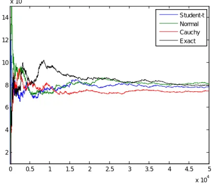
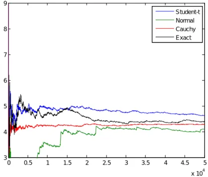
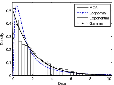
is given by fX(x/p), and cumulative distribution function (CDF), where p refers to the distribution parameters of the random variable X (continuous random variable), and x is a realization of X. For discrete random variable, a sample space is firstly defined which relates to the set of all possible outcomes, each element of the sample space is assigned a probability value between 0 and 1, and the sum of all the elements in the sample space to the “probability” value is called probability mass function (PMF). In the context of a probabilistic approach, two difficulties are encountered. The first is the choice of the distribution type (normal, lognormal, etc.). The choice of distribution type is known from previous experiences, priori knowledge, or expert opinion, those are quite subjective. The second difficulty is lack of adequate data to estimate the distribution parameters with a high degree of confidence[14].
Fig 2 - 3 Examples of probability density function
Classical statistics-based frequentist methodology addresses the uncertainty in the distribution parameters by estimating statistical confidence intervals, which cannot be used further in uncertainty propagation, reliability analysis, etc. In contrast, Bayesian probability interprets the concept of probability as a measure of a state of belief or knowledge of the quantity of interest, not as a frequency or a physical property of a system. It specifies some prior probability subjectively[15] , and then updates in the light of new evidence or observations by means of statistical inference approach. In
11
this way it can combine pre-existing knowledge with subsequent available information and update the prior knowledge with uncertainties. With the capability of dealing with both aleotory and epistemic uncertainties, the Bayesian theory has been widely applied, especially in reliability engineering.
2.3.2 Evidence theory
Evidence theory (Dempster-Shafer theory, D-S theory) measures uncertainty with belief and plausibility determined from known information. For a proposition, lower and upper bounds of probability with consistent evidence are defined instead of assigning a precise probability[16]. The information or evidence to measure belief and plausibility comes from a wide range of sources (e.g., experimental data, theoretical evidence, experts’ opinion concerning belief in value of a parameter or occurrence of an event, etc.). Meanwhile, the evidence can be combined with combination rules[17] .
Evidence theory begins with defining a frame of discernment X, which includes a set of mutually exclusive “elementary” propositions. The elements of the power set 2X can be taken to represent propositions concerning the actual state of the system. Evidence theory assigns a belief mass to each element of the power set by a basic belief assignment function m: 2X→[0,1] which has the following two properties: the mass of the empty set is zero, and the mass of all the member elements of the power set adds up to a total of 1.
The mass m(A) express the proportion of all relevant and available evidence that supports the claim that the actual state belongs to A. The value of m(A) pertains only to A and makes no additional claims about any subsets of A, each of which has its own mass. From the mass assignments, a probability interval can be defined which contains the precise probability, and the lower and upper bound measures are belief (Bel) and plausibility (Pl) as Bel(A) ≤ P(A) ≤ Pl(A).
The belief Bel(A) is defined as the sum of mass of all the subsets of A, which represents the amount of all the evidence supporting that the actual state belongs to A, and the plausibility Pl(A) is the sum of mass of all the sets that intersect with A, which represents the amount of all the evidence that does not rule out that the actual state belongs to A:
12
𝐁𝐁𝐁(𝐀) = ∑𝑩/𝑩∈𝑨𝒎(𝑩) (2 - 1) 𝐏𝐁(𝐀) = ∑𝑩/𝑩∩𝑨≠∅𝒎(𝑩) (2 - 2)
The two measures are related to each other as
𝐏𝐁(𝐀) = 𝟏 − 𝐁𝐁𝐁(𝑨�) 𝐁𝐁𝐁(𝐀) + 𝐁𝐁𝐁(𝑨�) ≤ 𝟏 𝐏𝐁(𝐀) + 𝐏𝐁(𝑨�) ≥ 𝟏 (2 - 3) Where 𝐴̅ is the complement of A.
The evidence space is characterized with cumulative belief function (CBF) and cumulative plausibility function (CPF).
Evidence theory can deal with the problems both of aleatory and epistemic uncertainties flexibly with its evidence combination rules to update probability measures[18]. It is actually close related to probability theory. When the amount of available information increases, an uncertainty representation with evidence theory can approach that with probability theory [19],[20]. However, it also has limitations when handle highly inconsistent data sources, which may render the evidence combination rule unreliable. Anyway, it has been widely utilized and attracted great research interest in the fields of uncertainty-based information, risk assessment, decision making, and design optimization [21],[22].
2.3.3 Possibility theory
Possibility theory is introduced as an extension of the theory of fuzzy set and fuzzy logic, which can be used to model uncertainties when there is imprecise information or sparse data. The term fuzzy set is in contrast with the conventional set (fixed boundaries).
In possibility theory, uncertain parameters are not treated as random variables but as possibilistic variables, the membership function is extended to possibility distribution. It expresses the degree of an event can occur by analyst as subjective knowledge. Like evidence theory, possibility theory can deal with both the aletory and epistemic uncertainties[23] . Compared to probability theory, possibility theory can be more conservative in terms of a confidence level. Because the knowledge of the analyst can be easily introduced to the design process and make problems more tractable[ 24 ] . The application of fuzzy set and possibility theory is feasible in
13
engineering design optimization and decision making. Fractile approach, modality optimization approach and spread minimization approach also be developed to solve possibilistic programming problems[25] . Possibility theory can also be applied along with probability theory, the integrated or unified algorithms are necessary to research and exploded[26], [27], [28], [29], [30] .
2.3.4 Interval analysis
Interval analysis is an approach to putting bounds on rounding errors and measurement errors in mathematical computation, and yield reliable results by developing numerical methods. In interval analysis the value of a variable is replaced by a pair of numbers representing the maximum and minimum values that the variable is expected to take. Interval arithmetic rules are applied to perform mathematical operations with the interval numbers, therefore the propagation of the interval bounds through the computational model is implemented, and the bounds on the output variables are achieved[31],[32],[33],[34].
2.3.5 Convex modeling
Convex modeling is a more general approach to represent uncertainties with convex sets[35]. The convex models include energy-bound model, interval model, ellipsoid model, envelope- bound model, slope- bound model, Fourier-bound model, etc. It is unlikely that the uncertain components are independent with each other and the bounds on the components of the object are reached simultaneously. Therefore, it is more reasonable to apply the convex model with representation of correlations between uncertain components in realistic application. In addition, techniques in interval analysis can be used here, when the convex models are intervals[36],[37]. Besides the foregoing five theories, there are other alternative approaches to represent uncertainties, especially for epistemic uncertainty[38], such as cloud theory mediating between fuzzy set theory and probability distribution, fuzzy random theory and random fuzzy theory with characteristics of both fuzzy set theory and probability theory[39] ,[40].
2.4 Model validation
In uncertainty based design, uncertainty representation models also have model form uncertainties, especially probabilistic models whose distributions are assumed and
14
fitted based on past experience, expert opinions, experimental data, etc. Hence, it is also necessary to measure the uncertainty of the model to validate the feasibility of the uncertainty representation[41].
Model form uncertainty can be characterized through model accuracy assessment by comparison between simulation results and experimental measurements. This process is also called model validation. It can be determined when the mathematical model of a physical event is sufficiently reliable to represent the actual physical event in the real practice.
To discuss whether a specific distribution is suitable to a data-set, the goodness of fit criteria can be applied. It includes the Pearson test[42], the Kolmogorov-Smirnov test[ 43], the Anderson-Darling test[ 44], etc. When the data available to test the hypothesis about probabilistic models are too scarce to allow definite conclusions to choose or discard totally one model among others, Bayesian method can be applied. It has the capability of combining several competing probability distribution types together to describe a random variable. More generally, a complete Bayesian solution is proposed to average over all possible models which can provide better predictive performance than any single model accounting for model uncertainties. When sampling from random vectors, it is important to control correlation or even dependence patterns between marginal. The bounds on the correlation errors can be useful for the selection of stopping criteria in algorithms employed for correlation control. In order to quantify an error in the correlation of a given sample, one must select a correlation estimator and define a scalar measure of the correlation matrix. Another goal of controlled statistical sampling is usually to perform the sampling with the smallest possible sample size, and yet achieve statistically significant estimates of the response.
The estimated correlation matrix is a symmetric matrix of the order Nvar and can be written as the sum
T
A= + +I L L (2 - 4) Where I is the identity matrix and Lis the strictly lower triangular matrix with entries with the range −1,1 . There are Nc correlation that describe pairwise correlations:
15
var var( var 1)
2 2
c
N N N
N = = −
(2 - 5)
2.4.1 Pearson correlation coefficient
The most well-known correlation measure is the linear Pearson correlation coefficient (PCC)[45]. The PCC takes values from between -1 and +1, inclusive, and provides a measure of the strength of the linear relationship between two variables. The actual PCC between two variables, say Xi and Xj , is estimated using the sample correlation coefficient Aij as , j, 1 2 2 , j, 1 1 (x X )(x X ) (x X ) (x X ) sim sim sim N i s i s j s ij N N i s i s j s s A = = = − − = − −
∑
∑
∑
(2 - 6) , 1 1 X x sim N i i s s sim N = =∑
, j, 1 1 X x sim N j s s sim N = =∑
(2 - 7)When the actual data xi,s , s=1, 2,,Nsim of each vector i=1, 2,,Nvar are
standardized into zi,s into vectors that yield zero average and unit sample variance estimates, the formula simplifies to
i, j, 2 2 , j, s s ij i s s r r A r r =
∑
∑ ∑
(2 - 8) i, j, 1 1 Nsim ij s s s sim A z z N = =∑
(2 - 9)Which is the dot product of two vectors divided by the sample size.
2.4.2 Spearman correlation coefficient
The formula for Spearman correlation coefficient[46] estimation is identical to the one for Pearson linear correlation with the exception that the values of random variables
i
16
permutation of numbers. It is convenient to transform the ranks into ri s, =
π
s,i−π
i andj,s s, j j r =
π
−π
. 1 1 1 2 sim N sim i j s sim N s N π π π = + = = =∑
= (2 - 10) The rank correlation is then defined as,i, j, 2 2 , j, s s ij i s s r r A r r =
∑
∑ ∑
(2 - 11)By noting that the sum of the first Nsim squared integers is ( 1)(2 1)
6
sim sim sim
N N + N + , we find that 3 2 2 , j, 12 sim sim i s s N N r = r = −
∑
∑
, and the rank correlation reads:i, j, i, j, 2 3 12 12 1 3 ( 1) 1 s s s s sim ij
sim sim sim sim sim
r r N A N N N N N π π + = = − − − −
∑
∑
(2 - 12)In the case of ties, the averaged ranks are used. Note that when LHS is applied to continuous parametric distributions no ties can occur in the generated data. Therefore, we do not consider ties from here on. Another formula exists for Spearman correlation suitable for data with no ties. The correlation coefficient between any two vectors each consisting of permutations of integer ranks from 1 to
sim N is 2 6 1 ( 1) ij sim sim D A N N = − − (2 - 13)
Where D is the sum of values ds, the differences between the th
s integer elements in the vectors: 2 1 sim N s s D d = =
∑
(2 - 14)17
Every mutual permutation of ranks can be achieved by permuting the ranks π of the s second variable against the identity permutation corresponding to the ranks of the first variable. Therefore, we may write
2 2
1 1 1
(s ) 2 s (s )
sim sim sim
N N N s s s s s D π π = = = = − = −
∑
∑
∑
(2 - 15) This is equal to 1 ( 1)(2 1) 2 (s ) 3 sim Nsim sim sim
s s N N N π = + + −
∑
(2 - 16)Spearman correlation can, in general, take any value between -1 and 1, inclusive, depending on the value of the sum 2
s
d
∑
. The lowest correlation is achieved for the reverse ordering of rank numbers and corresponds to the case when the sum D equal 2 ( 1) 3 sim sim N N −. Conversely, the maximum correlation is achieved for identical ranks and the sum equals zero.
2.4.3 Kendall correlation coefficient
Kendall’s correlation[47] (nonparametric or distribution-free) coefficient estimates the difference between the probability of concordance and discordance between two variables, xi and xj. For data without ties, the estimate is calculated based on the rankings π and i
π
j of Nsim samples of two vectors xi and xj. Let us index the ranks by 1≤k l, ≤Nsim . The formula for sample correlation is a direct estimation of the difference between the probabilities:, ,l j, j,l sgn ( )( ) 2 2 sim N i k i k c d k l ij sim sim n n A N N π π π π < − − − = =
∑
(2 - 17)Where sgn(z)= −1 for negative z, +1 for positive z, and zero for z =0.
The numerator counts the difference between concordant pairs nc and discordant pairs nd. The denominator is the maximum number of pairs with the same order, the
18
total number of item pairs with respect to which the ranking can be compared. The number of concordant pairs nc is the number of item pairs on the order of which both rankings agree. A pair
(
πi k, ,πj k,)
and(
πi,l ,πj,l)
of points in the sample is concordant if eitherπ
i,k <π
i,l andπ
j,k <π
j,l orπ
i,k >π
i,l andπ
j,k >π
j,l. Analogically, nd is thenumber on which both ranking disagreed.
The number of concordant pairs can be calculated by adding scores: a score of one for every pair of objects that are ranked in the same order and a zero score for every pair that are ranked in different orders:
, ,l j, j,l 1 ( )( ) 0 1 1 (l ) sim sim i k i k N N c k l k n π π π π − − − > = = + =
∑ ∑
(2 - 18)Where the indicator function lA equals one if A is true, and zero otherwise.
Analogically, nd would count only for opposite orders and the formula would be identical but with opposite orientation of the inequality sign.
In the cases of tied rank, the denominator is usually adjusted. We do not consider ties. Therefore, Aijcan be rewritten by exploiting the fact that the number of pairs is
the sum of concordant and discordant pairs and therefore the number of discordant pairs is 2 sim d c N n = −n . Then, 4 4 1 1 ( 1) ( 1) c d ij
sim sim sim sim
n n
A
N N N N
= − = −
− − (2 - 19)
A straightforward implementation of the algorithm based on the above equations has
2 ( N )sim
ϑ
complexity. In practice, it is convenient to rearrange the two rank vectors so that the first one is in increasing order.Kendall’s correlation coefficient is intuitively simple to interpret. When compared to the Spearman coefficient, its algebraic structure is much simpler. Note that Spearman’s coefficient involves concordance relationship among three sets of observation, which makes the interpretation somewhat more complex than that for
19
Kendall’s coefficient. Regarding the relation between Spearman’s correlation (ρ ) and Kendall’s correlation (
τ
)2 2
(1 ) 3 2 (1 )
τ − −τ ≤ τ− ρ τ≤ + −τ (2 - 20)
For many joint distribution, correlation coefficients of Spearman and Kendall have different values, as they measure different aspects of the dependence structure. It has long been known about the relationship between the two measurements that, for many distributions exhibiting weak dependence, the sample value of Spearman’s is about 50% larger than the sample value of Kendall’s.
2.5 Sensitivity analysis
Sensitivity analysis is the study of how the variation in the model output can be apportioned, qualitatively or quantitatively, to different sources of variations in the model input[ 48 ]. By means of this technique, uncertainty factors can be systematically studied to measure their effects on the system output, so as to filter out the uncertainty factors with negligible contributions and reduce complexity. With this specific aim, sensitivity analysis in this context is also termed uncertainty importance analysis.
There are numerous approaches to address sensitivity analysis under uncertainty, especially with probability theory. Probabilistic sensitivity analysis methods mainly include differential analysis, response surface methodology, variance decomposition, Fourier amplitude sensitivity test, sampling-based method[ 49 ], etc. Among these approaches, sampling-based method is widely applied for its flexibility and ease of implementation.
Once the sample is generated, evaluation of f created the following mapping from analysis inputs to analysis results
[
xi , y ,i]
i=1, 2,,nSWhere yi = f x( )i
20 1 (y) nS i i i E y w = =
∑
(2 - 21)[
]
2 1 (y) (y) nS i i i V E y w = =∑
− (2 - 22)The mapping in
[
xi , y ,i]
i=1, 2,,nS can be explored with various techniques to determine the effects of the individual elements of x on y.Differential analysis is based on the partial derivative of f with respect to the elements of
x
. In its simplest form, differential analysis involves approximating the model by the Taylor series0 0 0 1 y(x) f(x ) (x ) nX j j j j f x x x = = +
∑
∂ ∂ − (2 - 23)Where x0 = x , x10 20,, xnX,0 is a vector of base-case values for the xj.
One the approximation in the model of Taylor series is determined, variance propagation formulas can be used to determine the uncertainty in ythat results from the distribution. In particular,
0 0 0 1 (y) y(x ) (x ) nX j j j j E f x E x x = = +
∑
∂ ∂ − (2 - 24)[
]
2 0 0 0 1 1 1 (y) (x ) ( ) 2 (x ) (x ) ( , ) nX nX nX j j j k j k j j k j V f x V x f x f x Cov x x = = = + =∑
∂ ∂ +∑ ∑
∂ ∂ × ∂ ∂ (2 - 25) Thus, the Taylor series leads to approximations of the expected value and variance for y that result from the distributions. Sensitivity analysis is based on the use of partial derivatives associated with a Taylor series to determine the effects of the individual elements. If the elements are independent, then the fractional contribution of xj to the variance of y can be approximated by2 0
( j) (x ) j ( )j ( )
21
2.6 Uncertainty propagation
Uncertainty analysis is concerned with quantifying uncertainty characteristics of output in the system resulted from model input uncertainties and model uncertainties propagated through computational simulation. Generally uncertainty analysis approaches can be categorized into two types: intrusive and non-intrusive[50].
The intrusive type is mainly related to the physics-based approaches. It involves reformulation of governing equations and modification to the simulation codes so as to incorporate uncertainty directly into the system[51]. Typical example of this type is Polynomial Chaos expansion based approaches, which represent a stochastic process with expansion of orthogonal polynomials. The coefficient of the expansion can be defined by substituting the stochastic process with its polynomial chaos expansion in the original governing equations, which results in a coupled system of deterministic equations to be solved by editing the existing analysis codes.
In contrast to intrusive approaches, non-intrusive approaches treat computer simulation model as black-box and need no modification to existing deterministic simulation codes. So it can be developed for general use and take the advantage of being applicable to legacy codes. With this merit, the preceding Polynomial Chaos expansion based methods are also studied to be solved with non-intrusive approaches. Widely used non-intrusive approaches, include Monte Carlo simulation method, Taylor series approximation method, and some methods specific for reliability analysis[52]. Considering the computational difficulty in application of the conventional uncertainty analysis methods, decomposition based methods are introduced, which can treat uncertainty cross propagation among complex coupling disciplines more efficiently by decomposing the system uncertainty analysis problem into subsystem or disciplinary level.
2.6.1 Monte Carlo simulation
Monte Carlo simulation (MCS) methods (sampling-based methods) are a class of computational algorithms that perform repeated sampling and simulation. If sufficient samples are provided, MCS methods can provide statistical analysis results with arbitrary level of accuracy[53].
22
MCS is often used as a benchmark for evaluating the performance of new uncertainty analysis techniques. Lots of efforts have been devoted to develop approximation approaches to numerically evaluate this integral[54].
Gauss quadrature approaches and other numerical quadrature and cubature methods are proposed to approximate the multi-dimensional integral with weighted sum of the integrand values at a set of discrete integration points within the integration region. Laplace Approximation approach is proposed to approximate the integrand with second order Taylor series expansion at its minimum so as to derive the integral. Unfortunately, these approximate numerical integration approaches are generally only efficient and accurate for a special type of problem, quadrature based method for polynomial response, and may be not applicable especially for problems with high dimensional uncertainties and complex integrand which has no explicit formula and can only be calculated with time-consuming simulation analysis[55]. The difficulties with the traditional numerical integration approaches as motivation to the development of simulation based MCS integration methods, statistics of the system response by simply performing repeated sampling and simulation can be computed.
The disadvantage of MCS methods is computational prohibitive when simulation model is complex. For problems need iterations of several coupled disciplinary simulations to reach a consistent system response result, the situation becomes even worse[56]. To be more efficient than the random sampling method, several improved MCS methods with different sampling techniques have been developed and proved. Among these sampling methods, importance sampling (weighted sampling)[57], is pervasively studied. It is expected to reduce error to zero if importance sampling probability density function is correctly selected. However, in realistic engineering problems, generally theoretical optimum importance sampling functions are not practical.
A compromise method is Latin hypercube sampling (LHS) approach[ 58 ]. This approach divides the range of each variable into disjoint intervals of equal probability, and one value is randomly selected from each interval. It improves MCS stability and also maintains the tractability of random sampling.
23
The first-order sensitivity method, as a variance reduction technique, is also utilized to accelerate MCS estimation convergence[59]. It is observed that this sensitivity enhanced method can improve accuracy by one order of magnitude compared to error. The variance reduction techniques are especially important when MCS is applied to estimate small failure probability.
2.6.2 Taylor series approximation
Taylor series approximation methods have been widely used for the relative ease of understanding and implementation[ 60 ]. This method can be employed to approximate statistical moments of system output based on partial derivatives of the output f with respect to the elements of the random input vector x. The original simulation model function y=f(x) can be approximated with the first order Taylor series as,
+𝐲(𝐱) ≈ 𝐟(𝐱𝐱) + � �𝒏𝒌�𝒙𝒌𝒂𝒏−𝒌
𝒏
𝒌=𝐱 (2 - 27)
Where x0 is the base point vector at which the derivatives are calculated. The output uncertainty resulting from the random input uncertainties can be determined with uncertainty propagation through this approximation formula.
Taylor series approximation methods have several disadvantages[61]:
(1) Its estimation accuracy is low when the coefficients of variation of the input random vector increase.
(2) The increase of Taylor series expansion order leads to rapidly increase of estimation complexity due to high-order terms and correlations between the elements.
(3) The determination of partial derivatives could be very difficult for complex system simulation models.
As Taylor series approximation methods only deal with the propagation of first two moments rather than the exact distribution of randomness, it belongs to first-order, second-moment methods which are related to the class of problems only concerning the means and variances and their propagation. This is a logical naming convention for the uncertainty propagation techniques with a given choice of the order of approximation and the statistical moment to be used [62]. Besides Taylor series
24
approximation methods, there are also several other first order, second-moment approaches such as point-estimate-for-probability-moment methods.
2.6.3 Reliability analysis
Reliability of the system is generally difficult to calculate analytical as both the joint probability distribution function p(x) and the failure domain D are seldom accurately defined in an explicit analytical form, and the multidimensional integration can be computationally prohibitive especially for the complex system with time consuming analysis models[ 63 ]. Hence, it is motivated to develop various approximation methods, including the preceding numerical integration methods, as well as other integration approximation methods specific for reliability analysis. Laplace multidimensional integral method based asymptotic approximation, main domain of failure coverage base integration, fast Fourier transform (FFT) based method, tail modeling approach, dimension-reduction (DR) methodology, First Order Reliability Method (FORM) and Second Order Reliability Method (SORM), etc[ 64 ]. Among these approximation methods, FORM and SORM are most prevailing and wide applied in engineering problems.
To further improve reliability analysis efficiency, response surface methodology (RSM) can be utilized to replace the computationally expensive accurate function so as to reduce calculation burden[65]. Interval analysis, possibility theory, evidence theory and convex uncertainty in reliability analysis are also studied. Besides the methods to determine exact reliability, there are also some approaches dealing with reliability bounds.
2.6.4 Decomposition based uncertainty analysis
For a complex system with close coupled disciplines, tremendous repeating multidisciplinary analysis (MDA), Monte Carlo methods, FORM/SORM make uncertainty analysis computationally prohibitive. As a solution to this problem, decomposition strategies are proposed to decompose the uncertainty analysis problem nested with MDA into several discipline or subsystem uncertainty analysis problems, so as to control each sub-problem within acceptable level and meanwhile take advantages of distributed parallel computing[66].
For MPP based uncertainty analysis, the search procedure of MPP is essentially a double loop algorithm, which includes a MPP search optimization in the outside loop
25
and a MDA iteration procedure in the inner loop. To improve the search efficiency of MPP, decomposition based approaches have been suggested[ 67 ]. In addition, employing concurrent subspace optimization (CSSO) procedure to solve the MPP search optimization problem, so called MPP-CSSO, also greatly improve efficiency with parallelization of disciplinary analysis and optimization [61].
Last but not the least, another solution to address the double loop problem is to decompose MDA from the MPP search and organize them sequentially as a recursive loop. In this sequential approach to reliability analysis for multidisciplinary systems (SARAM), concurrent subsystem analysis can be applied in the separate MDA to further alleviate computational burden [61].
For numerical simulation based reliability analysis, Gibbs sampling[68] is utilized to decompose MDA into disciplinary sub-problems and reduce the consistency of multidisciplinary system at each run. Without consistency constraint on MDA, only the number of disciplines times the disciplinary analysis computation are needed for each run of sample simulation, which can greatly reduce calculation cost compared to the traditional sampling method that needs iterations of disciplinary analysis to obtain a consistent system response at each sample.
2.7 Conclusion
In this chapter, we first discussed the uncertainty classification and sources of uncertainty in numerical simulation. Probability theory, evidence theory, possibility theory, interval analysis and also convex modeling are reminded as theory of uncertainty representation and modeling for uncertainty analysis. To take consideration of in uncertainty representation models it is also necessary to validate the feasibility of the uncertainty representation by Person correlation, Spearman correlation or Kendall correlation.
Sensitivity analysis, also termed uncertainty importance analysis, analyse the influence effect of different sources of variations in the model input to variation in the model output. It can filter out the uncertainty factors with negligible contributions and reduce complexity as discussed in fifth section of this chapter. Quantifying uncertainty characteristics of output in the system resulted from model input uncertainties and model uncertainties propagated through computational simulation
26
are the key problems in uncertainty analysis, we discussed it in the last section of this thiese.
27
Chapter 3 Monte Carlo Simulation
Monte Carlo sampling got its name as the code word for work that von Neumann and Ulam were doing during World War II on the Manhatten Project at Los Alamos for the atom bomb where it was used to integrate otherwise intractable mathematical functions[69] (Rubinstein, 1981). However, one of the earliest examples of the use of the Monte Carlo method was in the famous Buffon's needle problem where needles were physically thrown randomly onto a gridded field to estimate the value of p. In the beginning of the 20th century the Monte Carlo method was also used to examine the Boltzmann Equation and in 1908 the famous statistician Student (W.S. Gossett) applied the Monte Carlo method for estimating the correlation coefficient in his t-distribution[70].
A basic advantage of sampling methods is their direct utilization of experiments to obtain mathematical solutions or probabilistic information concerning problems whose system equations cannot be solved easily by known procedures[ 71 ]. Application of Monte Carlo Method to probabilistic structural analysis problems is comparatively recent, becoming practical only with the advent of digital computers. It is a powerful mathematical tool for determining the approximate probability of a specific event that is the outcome of a series of stochastic processes.
3.1 Mathematical formulation of Monte Carlo Integration
The quality of any algorithm that approximate the true value of the solution depends very much of the convergence rate. One needs to estimate how fast the approximate solution converges to the true solution. Let ξ be a random variable for which the mathematical expectation of E( )ξ =I exists. Formally defined as,
( ) ( ) 1 . .
( )
( ) ( ) 1 . .
x
p d where p x dx when is a continuous r v E
p where p x when is a discrete r v
ξ ξ ξ ξ ξ ξ ξ ξ ξ ∞ ∞ −∞ −∞ = = =
∫
∫
∑
∑
(3 - 1)The nonnegative function p x( ) (continuous or discrete) is called the probability density function. To approximate the variableI , a computation of the arithmetic mean must usually be carried out,
28 1 1 N N i i N ξ ξ = =
∑
(3 - 2)For a sequence of uniformly distributed independent random variables, for which the mathematical expectation exists, the theorem of J. Bernoulli[72] ( who proved for the first time the Law of Large Number Theorem) . This means that the arithmetic mean of these variables converges to the mathematical expectation:
p
N I as N
ξ → → ∞
The sequence of the random variables η η1, 2,,ηN , converges to the constant
c
if for everyh>0, it follow that,
{
}
lim N 0
N→∞P η − ≥c h =
Thus, when N is sufficiently large
ξ
N ≈ISuppose that the random variable ξ has a finite variance, the error of the algorithm can be estimated as,
2 2 2
( ) [ ( )] ( ) [ ( )]
D ξ =E ξ−E ξ =E ξ − E ξ (3 - 3)
3.1.1 Plain (crude) Monte Carlo Algorithm
Crude Monte Carlo is the simplest possible approach for solving multidimensional integrals. This approach simply applied the definition of the mathematical expectation. Let Ω be an arbitrary domain and d
x∈Ω ⊂R be a d-dimensional vector.
We consider the problem of the approximate computation of the integral
( ) ( )
I f x p x dx
Ω
=
∫
(3 - 4)Where the non-negative function p x( ) is density function p x dx( ) 1
Ω =
∫
.Let ξ be a random point with probability density function p x( ). Introducing the random variable
= ( )f
29
With mathematical expectation equal to the value of integral I
( ) ( ) ( )
E θ f x p x dx
Ω
=
∫
(3 - 6)Let the random points ξ ξ1, 2, ... ,ξ be independent realizations of the random point N ξ with probability density functionp x( ), then an approximate value of I is
1 1 N N i i N θ θ = =
∑
(3 - 7) If 1 1 N N i i N ξ ξ ==
∑
were absolutely convergent, thenθ
N would be convergent toI .3.1.2 Geometric Monte Carlo Algorithm
Let the nonnegative function f be bounded, 0≤ f x( )≤c for x∈ Ω
Where
c
is a generic constant. Consider the cylindrical domain[0, ]c
Ω = Ω×
And the random point ξ=(ξ ξ ξ1, 2 , 3)⊂ Ω with the following probability density function 1 2 1 ( ) ( , ) p x p x x c = (3 - 8)
Let ξ1,... ,ξ be independent realization of the random pointN
ξ
. Introduce the random variable 3 1 2 3 1 2 , ( , ) = 0 , ( , ) c if f if f ξ ξ ξ θ ξ ξ ξ < ≥ (3 - 9)The random variable introduced is a measure of the points below the graph of the function f .
30
{
}
1 2 3 ( , ) 1 2 0 1 2 3 3 ( ) Pr ( ) ( , , ) f x x E c f dx dx p x x x dx I θ ξ ξ Ω = < =∫
∫
= (3 - 10)The algorithm consists of generating a sequence of random points uniformly distributed in the third direction and accepting points if they are under the graph of the function and rejecting other points. This is the reason to call this Geometric algorithm an acceptance-rejection technique.
Compare the accuracy of the Geometric and the Plain Monte Carlo algorithm
Let f ∈L2( , )Ω p guarantees that the variance
2 2
( ) ( ) ( )
Dθ f x p x dx I
Ω
=
∫
− in a Plain Monte Carlo algorithm is finite.
For the Geometric Monte Carlo algorithm the following equation holds
{
}
2 2 3
( ) P ( )
E θ =c x < f ξ =cI (3 - 11) Hence the variance is D( )
θ
= −cI I2. Because2
( ) ( ) ( ) ( )
f x p x dx c f x p x dx cI
Ω ≤ Ω =
∫
∫
(3 - 12)Therefore, D( )
θ
≤D( )θ
. The last inequality shows that the Plain Monte Carlo algorithm is more accurate than the Geometric one (except for the case when the function f is a constant). Nevertheless, the Geometric algorithm is often preferred, from the algorithmic point of view, because its computational complexity may be less than that of the plain algorithm.3.2 Advanced Monte Carlo Methods
The probable error in Monte Carlo algorithms will appear when no information about the smoothness of the function is used
N D r c N ξ = (3 - 13)
It is important for such computational schemes and random variables that a value of
31
reduced variance compared to Plain Monte Carlo algorithms are usually called advanced Monte Carlo algorithms. Consider the integral
( ) ( )
I f x p x dx
Ω
=
∫
(3 - 14)Where f ∈L2( , ) ,Ω p x∈Ω ⊂Rd
Let the function h x( )∈L2( , )Ω p be close to f x( ) with respect to its L2 norm;
2 L
f −h ≤ . The value of the integral is supposed as ε
( ) ( )
I h x p x dx I
Ω ′
=
∫
= (3 - 15)The random variable θ′= f( )ξ −h( )ξ +I′ generates the following estimate for the integral 1 1 [ ( ) ( )] N N i i i I f h N θ ξ ξ = ′ = +′
∑
− (3 - 16)A possible estimate of the variance of
θ
′ is2 2 2
( ) [ ( ) ( )] ( ) ( )
Dθ f x h x p x dx I I ε
Ω
′ =
∫
− − − ′ ≤ (3 - 17)This means that the variance and the probable error will be quite small, if the function ( )
h x is such that the integral I ′ can be calculated analytically. The function h x( ) is often chosen to be piece-wise linear function in order to compute the value of I ′ easily.
3.2.1 Importance Sampling Algorithm
Importance sampling is a variance reduction technique that can be used in the Monte Carlo method. The basic idea behind importance sampling is that certain values of the input random variables in a simulation have more impact on the parameter being estimated than others. If these "important" values are emphasized by sampling more frequently, then the estimator variance can be reduced. Hence, the basic methodology in importance sampling is to choose a distribution which "encourages" the important values.