HAL Id: hal-01212617
https://hal.archives-ouvertes.fr/hal-01212617
Submitted on 14 Oct 2015HAL is a multi-disciplinary open access
archive for the deposit and dissemination of sci-entific research documents, whether they are pub-lished or not. The documents may come from teaching and research institutions in France or abroad, or from public or private research centers.
L’archive ouverte pluridisciplinaire HAL, est destinée au dépôt et à la diffusion de documents scientifiques de niveau recherche, publiés ou non, émanant des établissements d’enseignement et de recherche français ou étrangers, des laboratoires publics ou privés.
Formal DEVS modelling and simulation of a Flow-Shop
relocation method without interrupting the production
Patrick Pujo, Massimo Pedetti, Norbert Giambiasi
To cite this version:
Patrick Pujo, Massimo Pedetti, Norbert Giambiasi. Formal DEVS modelling and simulation of a Flow-Shop relocation method without interrupting the production. Simulation Modelling Practice and Theory, Elsevier, 2006, 14, pp.817-842. �hal-01212617�
Formal DEVS modelling and simulation
of a Flow-Shop relocation method
without interrupting the production
Patrick Pujo
1, Massimo Pedetti, Norbert Giambiasi
Research Group in Control and Simulation Laboratoire des Sciences de l’Information et des Systèmes
UMR CNRS 6168
Avenue Escadrille Normandie Niemen, F-13397 Marseille cedex 20, France
Abstract
This paper presents an organisational method to keep the production going during the removal of a flow-shop. Assume a flow-shop system is to be moved on a new site and its production has to continue, our method can be applied to follow requests for the removal period. The method works as follows: we segment the removals in groups of machines and move them ones after the others. This method can be successfully executed provided that a prime condition is met: envisaging sufficient stocks’ plug between each group. The role of the latter stocks is to ensure operations’ production continuity between the old and the new site, when the non-operational group is being removed. Removal is then renewed until the whole line is moved and is operational on the new site. To validate this approach, we have used simulation and developed a model of the flow-shop according to coupled DEVS formalism. Our model enables to segment a production line. As a consequence, we can simulate the sequential displacement of machines’ groups towards the new site. Among the solutions suggested, those starting with the final group (finished products) and while finishing with the first group are much more effective. In this paper, we present and discuss some simulation results of an industrial case study. The results demonstrate the compared effectiveness of various strategies of removal, and make possible for the industrialist to envisage a good estimated project management.
Keywords: Flow-shop relocation project management, Simulation, DEVS formalism, Facilities Relocation.
1. INTRODUCTION
The relocation of a production site is a difficult industrial project and many firms hesitate to get into this kind of trouble, especially small or medium sized companies that have to go
on operating with the same machines. A simple solution consists in removal during paid holidays: it is then possible to close the firm for the duration of the removal process. When a firm works on orders, without any annual closing, it needs to be continuously present on the market. It also needs a great ability to react making such strategies not conceivable. Although similar situations are commonplace, this problem has not been dealt with yet. We can consider the case of relocating the current facilities of a company to a nearby site. Two companies that were faced with the problem of removing a line of machines from one site to another without interrupting the production twice approached us. The constraints of the removal project were the same for both companies:
The production could not be stopped completely during the removal of the machines, The removal process was of flow-shop type,
The budget of the removal operation was limited, which forbade any solution of flash removal type (removal the totality of the production system overnight or during a weekend),
The global production process remained identical, i.e. logical chain of the operations remained the same (the same machines would continue to be used one after the other). This unusual problem is not dealt with in reference books about production organization [2, 9] or facilities planning [26]. Even the fundamental book on methods of facilities layout [17] does not deal with the organization of removal faced with such constraints. Recent papers have focused on facilities relocation. In fact, these articles deal with location or layout strategies, by considering mathematical approaches [3, 12, 15, 5] or by proposing oriented management methods [24, 19, 20, 16].
However, the removal organization problem is not dealt with in these papers.
In this context, and as a consequence, we have elaborated an organizational method to keep production going during the removal of a flow-shop. We propose here a solution of progressive removal of the resources to the new site by segmenting the whole production line in sub-sets and building up a buffer stock for each elementary removal of a sub-set. The true problem lies in the choice of the good parameters to balance the relocation organisation. A great number of solutions can be planned to segment the totality of the production line. The use of simulation in the field of manufacturing systems for simplifying the complexity and reducing the problem dimension is recognised by scientists and industrial managers. In our case, simulation aims at determining the best values combination of input parameters, given an output criterion [21].
In this paper, attention is focused on DEVS modelling for the relocation problem. The paper is structured as follows. Section 2 describes the relevance of the DEVS formalism for manufacturing systems’ simulation. Section 3 presents theoretical considerations for an elementary removal of a production workstation. Section 4 is devoted to the description of the relocation organisation of the complete production line. We use a case study and different simulations to test various strategies about the removal organization of the complete line. Section 5 describes an industrial case of printed-circuit boards’ production line, working on orders. The DEVS models are provided. Section 6 analyses simulation experiments’ results that the company can use to choose the best relocation strategy.
2. DEVS APPLICATION FOR MANUFACTURING SYSTEMS SIMULATION In this section, the manufacturing systems’ simulation issue is presented. First, the general characteristics of industrial engineering problems are described. Then, the DEVS formalism concept is introduced and its advantage exposed.
2.1. The issue of manufacturing systems’ simulation
Manufacturing systems are regarded as complex systems. As such, various problems arise in the comprehension of their operation, their dimensioning or the evaluation of their performance. These problems are seldom solved by an analytical approach, such as operations research approaches. Indeed, the latter produce models based on relations between various variables in order to seek an optimal configuration of their values. In fact there are two specific factors in production systems that prevent the use of operations research techniques. Firstly, production systems are discrete events systems. Time is one of the principal components in the search for the solution. The temporal constraints are expressed in the form of connected inequations. Their number is equal to the number of events. Secondly, these events are not perfectly known in advance: the events dates rise from various lengths of time duration. It is all about manufacture, transport and/or assembly tasks, which are only known with a quite relative precision. Moreover, unforeseen events can occur, in a random and perturbing way. This contingency of the events implies that a solution obtained by operations research techniques is often only a valid solution with respect to an idealized behavior of the production system. However, discrete events systems can be particularly well studied by simulation. Simulation enables to reproduce production systems’ dynamic evolution according to the above-mentioned uncertainties (using stochastic modeling). The dynamic behavior of the system is then described according to its evolution logic: progress of state changes and events generations. This is of course contextual, i.e. the evolution depends above all on the present state. In fact, this evolution logic is examined at each occurrence of event, step by step. This enables to manage the evolution of future event lists. These events are then qualified by the endogenous ones, i.e. they are the consequence of system state changes. Other events can be exogenous; i.e. the external environment of the system generates them. Their occurrence can be described explicitly (such as a list of dates of external events) or implicitly (using any probability distribution). For all events types, it is the behavior of the considered entity in the real world, which enables to formalize the simulation model. An activity is defined, when the time duration has a specified length, i.e. ‘know when it begins’ (unconditional wait), and a delay, when the time duration has an unspecified or indefinite length, i.e. ‘not know until it ends’ (conditional wait).
Fishwick [7] lists the advantages of using simulation models and methodology for modelling manufacturing systems as follows:
- Simulation models are more simple to determine than analytic models,
- Realistic models (complex systems representation) can be construct, whereas analytic models require simplifying assumptions,
- Performance measures to estimate the system behavior are easy to obtain, and visual output gives a good assistance to the end-user,
These advantages imply that simulation is used in FMS [13], to improve its control [23]. 2.2. Advantages of DEVS formalism applications
The Discret EVent system Specification (DEVS) formalism was developed by Zeigler to model and simulate discrete events dynamic systems [27]. This system analysis with unified concepts facilitates the concise description of discrete event systems. DEVS enables the development of robust model representation, based on atomic models concepts and on higher-level models representation closed under coupling. This enables a hierarchical modelling, where atomic models are considered as black boxes.
DEVS is totally independent from the implementation of simulators that use such system’s modeling. Various DEVS applications can thus be quoted, in robotics, computer architectures, VLSI design, ecology modelling and analysis and environmental systems, amongst others. In transportation systems, Lee et al. [14] performed distributed
homogeneous traffic simulation by extending developed DEVS-based I3D2 transportation
simulation system to an HLA-based distributed environment. Nidumolu et al. [18] suggest that DEVS could be applied to simulate and evaluate complex business process models. These two examples have studied connected domains to operations’ management domain. In our laboratory, we have used DEVS to support the knowledge of control system behavior of iron-making blast furnace [8].
DEVS begin to be applied to industrial production systems. For example, Choi et al. [6] have developed a factory simulator, which can give virtual 3D representation of an automated manufacturing system by employing a job-resource relation network systematically converted to a DEVS model. Equivalent ideas were presented in [1], applied to a FMS plant.
We have shown [25] how simulation can be a useful tool for production systems control aid. The information given by the simulation allows a proactive control to be set up to anticipate blocked situations. This topic was illustrated in the paper by using the coupled DEVS formalism for a Kanban workstation modelling.
The major DEVS concepts can be founded in appendix 1. DEVS defines a method of abstraction of dynamic systems that allows building timed discrete event simulation models (deterministic models) with a good accuracy. DEVS is a symbolic specification of system semantics and there is only one way to execute a DEVS model.
Potential benefits may lie in the ability of DEVS
a) to implement event filtering, wherein a planned change of state will be realized by a model only when the time interval that separate two key events exceeds a predefined value, b) to encapsulate the otherwise mechanical event filtering at the conceptual level.
To our knowledge, only DEVS formalism offers all the concepts necessary to represent, at the conceptual level, phenomena such as filtering and autonomous evolution… phenomena that are described by expert and must be formally represented before implementation occur. The operative semantics of DEVS is clearly defined by the concept of conceptual simulator. Then, a DEVS specification is independent of the simulation technology as well as the underlying host computer. Thus, DEVS models can be translated in all commercial simulation software for manufacturing processes like Arena, AutoMod, eM-Plant, Taylor ED.
3. ELEMENTARY REMOVAL OF A WORKSTATION: CANONIC STUDY 3.1. Analysis of the modelling problem
In order to relocate a complete production line, an elementary pattern of how the production system will behave during removal is needed: we describe some of the theoretical facts obtained from the example of a sub-set composed of only one machine.
We call Mi the machine number i of a line of n machines. The machine, which is a removal
one, is noted k. We also note n i
i p C C 1 min
the production rate of the line, with Ci the
maximal production rate of the machine Mi, Si the products’ stock located upstream of this
machine and Qi the quantity of products in Si.
3.1.1. Analysis of the removal principle
As our removal principle is based on a succession of small removals (one machine after the other or a group of machines after the other), the same production line appears in all the project stages both on the old and the new production sites. The only exceptions are at the very beginning of the removal, when no machine has yet been moved, and at its end, when all the machines are at their proper places in the new site. Let us take a canonical example, where n=3 and k=2. In all the steady intermediate states, i.e. between two successive removals of two sub-sets, the logistic link between the two sites is ensured through a buffer stock. The buffer stock decouples the operation of the two sites and allows the parts’ transport between the sites (i.e. stock S3). The Work-In-Process (WIP) has to be dispatched to the new site, which generates an additional delay but does not challenge the management of the production system. During the removal of machine M2, the production system is modified.
Machine M1 maximum rate C1
Machine M2
maximum rate C2 maximum rate C3 Machine M3
Stock S1
level Q1 Stock S2 level Q2
input products output products Production System: production rate Cp Stock S3 level Q3 Stock S4 level Q4
old site new site
site 1.a. Model of a production line.
Production system: production rate Cp M1
Stock S1
level Q1 Stock S2 level Q2
raw materials M3 output products Stock S3 level Q3 Stock S4 level Q4
1.b. Model of an interrupted flow production line. Figure 1. Model of a production line during a removal.
Indeed, M2 is stopped during its removal and so there are two production lines: one downstream on the new site, and one upstream on the old site.
To keep on producing, while M2 is unavailable (i.e. as long as its removal lasts (tMov2)), the
level of the stock S3 has to be high enough to allow input in the next machine (M3). As for S2, it will be loaded progressively because there is no more consumption of WIP. To keep this line in operation while avoiding production discontinuities is thus linked to controlling the intermediate stocks S3 and S2. In the sequel, the required decision mechanisms are explained in detail.
3.1.2. Study of the downstream and upstream flow-shops
To ensure finished goods production’ continuity, M3 must go on producing during the removal of M2, i.e. S3 must contain a sufficient quantity of products to be able to feed M3 at the rate Cp during tMov2. This reserve quantity defined as Q 3 Cp*tMov2 is built up in a
period of time * Mov2
p up p t C C C t
, by increasing the upstream rate to the maximum upstream
rate Cup. Generally, i k i up C C 1 1 min
. This stock builds up while the upstream production goes
on as usual. During the removal of M2, the upstream part of the line can go on producing
as usual, thereby creating a stock in S2. The volume of this stock, defined as Q 2 Cp*tMov2,
will be absorbed in a time * Mov2
p dw p t C C C t
, where Cdw is the downstream maximum rate.
Generally, i n k i dw C C 1 min
. In a normal running situation, if M2 is already working with a
maximal rate, keeping the global rate of the production line is possible by stopping the entire production during this elementary removal. The latter will avoid creating undesirable stocks, which will not be absorbed afterwards.
3.2. DEVS model of an elementary removal of a production workstation In this section, the basic entities of the production line to be modeled are described. 3.2.1. Elementary model
The production line consists of an alternation of stocks, where parts, grouped by batches, are waiting to be transformed. It also consists of machines, where batches are treated part by part before returning to wait. Inputs at the beginning of the production line are raw materials, and outputs are finished goods.
The production line simulation with the DEVS formalism will keep this structure: figure 2a illustrates the model with the alternation of WS (the WorkStation) and BS (the Buffer Stock), where WS is the generic model of a machine and BS is the generic model of a stock, in order to obtain the coupled model by simulation of the complete line, arrows represent the links between these models.
2a. DEVS model of production line. BSi batchinbsi WSi capacitybsi batchoutbsi WSi batchinwsi inhibwsi batchoutwsi prodmodewsi BSi+1 batchinbsi+1 WSi+1 capacitybsi+1 batchoutbsi+1
2b. Coupling between buffer stocks models and workstation model. Figure 2. DEVS model of production line.
3.2.2. The 'WS' detailed model
A workstation is modelled using a generic model described in coupled DEVS with a set of particular parameters which values specify the operation mode. These models are then associated to the other workstation’s models to constitute the complete production line. The association of three functions builds each generic model of workstation: 'upstream interface', 'machine' and 'downstream interface'. We hereby provide an informal description of the generic model behavior.
When the production line is in a nominal state of operation, each workstation works batch by batch. A workstation begins to work when its upstream stock sends in a batch of C parts to be transformed. The reception of this batch by the workstation is made by the function 'upstream interface'. This machine interface enables to manage the parts of the batch one by one. It is thus about an un-stacking operation of the batch to present them to the transformation function 'machine'. After the treatment, each part of WIP is sent to the ‘downstream interface’, with the aim of reconstructing the batch part by part.
When the batch is completely treated, it is thus reconstituted in the ‘downstream interface’. This batch is then sent to the downstream buffer stock.
The workstation, which is now inactive, can then receive a new batch and begin again the previous process.
Note that we have described the workstation’s behavior mechanisms by considering the fact that a single batch is treated at the same time: the reception of a new batch is only possible when the treatment of the previous batch is finished by sending this latter in the downstream buffer stock.
raw material s finished goods WS BS BS WS BS WS BS WS
Such an operation is modeled using the DEVS model 'WS' in figure 3. 'WS' is a coupled DEVS model consisting of three atomic DEVS models, 'upstream interface', 'machine' and 'downstream interface'. Their behavior is respectively described in the next sections.
machine newWIPm WIPm WS upstream interface WIPui inhibui newWIPui batchinui prodmodeui downstream interface batchoutdi WIPdi 0 ; 1 prodmodews get batchinws refuse inhibws batchoutws send physical event informative event
Figure 3. 'WS': DEVS coupled model of workstation. 3.2.3. ‘Upstream interface’ detailed model
a: informal description of the behavior of ‘upstream interface’
The 'upstream interface' atomic model (figure 4a) can receive or reject batches, requests for parts and information on the operating mode. Two operating modes are available: normal production and stop during removal. The latter allows the machine to stop the production: it blocks the introduction of any new batch in the workstation, but permits to empty the workstation without interrupting the execution of the current batch.
Indeed, the signal to stop the production does not produce an immediate effect, but it enables to end the possibly present batch and to have a machine, which remains empty, even if there is, or not batches in wait in the upstream stock.
b: formal description in DEVS of ‘upstream interface’ model
‘upstream interface’ = <Xui, Yui, S, ext, int, , t>
Input event variables: Xui = (batchinui, WIPui, prodmodeui), where:
‘batchinui’ = {get} – this event indicates the arrival of a new batch,
‘WIPui’ = {done} – this event indicates the request for a new part,
‘prodmodeui’ = {0, 1} – this port gives the order for the operating mode of the
machine: the external event ?prodmodeui=’1’ indicates the ‘normal production’
operating mode; the external event ?prodmodeui=’0’ indicates the ‘stop during
removal’ operating mode.
State variables: S = {(phase, mode, job, sigma)}, where:
phase = {refuse, noprod, waitbatch, receive, queue, wait, lastbatch, lastqueue,
wait2}, is a name representing the situation in the real world,
mode={0, 1} is a variable that represents the operating mode, with the following
interpretation: mode=0 is the ‘stop during removal’ mode, mode=1 is the ‘normal
production’ mode (it is the default value),
job IN , is the counting variable of the parts (jobs) to be worked presents in the 0
sigma
0
IR , is the life time of the current state.
Output event variables: Yui = (inhibui, newWIPui), where:
inhibui = {refuse} – this event indicates that an incoming batch is not accepted,
newWIPui = {yes, no} – the output event !newWIPui='yes' indicates that there is
another part to be treated. The output event !newWIPui='no' indicates the absence of
part: finished batch or no batch in standby.
The functions of the 'upstream interface' DEVS model are described and defined using the graph in figure 4a:
batchinui get WIPui done prodmodeui 0 ; 1 inhibu i refuse newWIPui yes ; no upstream interface ' ' !newWIPuino ' ' !newWIPu iyes 0 job 0 job ' ' ?WIPu idone ' ' ?batchinuiget ' ' ?WIPuidone ' ' !newWIPuiyes wait2 mode job=job-1 infinite ' ' !newWIPuino ' ' ?WIPu idone ' ' !inhib refuse waitbatch mode=1 job=0 infinite receive mode job=job+C 0 queue mode job 0 wait mode job=job-1 infinite noprod mode=0 job=0 infinite normal production refuse mode job 0 lastqueue mode job 0 lastbatch mode=0 job infinite stop during removal internal transition external transition ' ' ?batchinuiget if if 0 job if 0 job if ' 0 ' ?prodmodeui ' 1' ?prodmodeu i ' 0 ' ?prodmodeui
4a. DEVS atomic model of ‘upstream interface’.
4b. DEVS atomic model of ‘machine’.
4c. DEVS atomic model of ‘downstream interface’. Figure 4. Internal DEVS atomic models of 'WS'.
WIPdi done
downstream interface batchoutsenddi
waitWIP worked=0 infinite receive worked= worked+1 0 ' '
?WIPmdone queue
worked infinite C worked if ' ' ?WIPmdone C worked if send batchoutdi ! WIPm done machine newWIPm yes; no waitnewWIP infinite work finite ' ' ?newWIPm yes ' ' !WIPm done ' ' ?newWIPm no
c: interpretation of DEVS model behavior
In figure 4a, displays on the right side the normal production conditions (normal production operating mode), where mode='1'. It displays on the left side the behavior during the removal (stop during removal operating mode), where mode='0'. Assume we are in the initial state with mode='1' and no WIP (job=0). The initial 'waitbatch' state is
passive (i.e. its life time is ). A transition occurs at the external event ?batchinui='get',
corresponding to the reception of a new batch. The arrival state 'receive' of this transition is transitory (i.e. its life time is 0): its role only consists in updating the number of parts in wait (in fact, the variable job, which was equal to 0, change its value to job+C, assuming C is the quantity of parts of the received batch). The following internal transition enables to begin the treatment of the batch: the arrival state 'queue', also transitory, enables to go into a loop of un-stacking until job nullifies. When job> 0, i.e. as long as there are parts to be worked (which is necessarily true just after the reception of a new batch), the sending of a
part towards the machine is activated (output !newWIPui='yes') during the transition
towards the passive 'wait' state, where the value of job decreases 1 (i.e. it passes from job to job-1). From the latter state, one returns to the state 'queue' during the external event
?WIPui='done'. This loop continues until the time occurrence when there are not parts
anymore in the batch (job=0), where we return to the initial state with an internal transition
corresponding to the output signal !newWIPui='no'.
For the external event ?prodmodeui='0', several cases are possible, depending on the
internal state of 'upstream interface'. If, for example, it occurs during the initial 'waitbatch' state (the workstation is empty), the model switches directly in the passive 'noprod' state, the value of mode switches from '1' to '0' and job remains equal to '0'. At this time
occurrence, it can receive a new batch (?batchinui='get'), but because of the inhibition, it
has to refuse it: there is a transition towards the transitory state 'refuse', which induces at
once the return of the system towards 'noprod' and the output signal !inhibui='refuse'. It is
also possible that it receives the order of the normal production operating mode with the external event ?m=1: it induces the transition towards the state 'waitbatch', and thus towards the normal conditions of operation.
If, on the contrary, the external event ?prodmodeui='0' occurs during the treatment of a
batch, it involves the state 'wait'. The passive state 'lastlot' is then reached, where job keeps
the same value as in 'wait', but where mode=0. The input signal ?WIPui='done', which
represents the free machine, induces the transition towards the transitory state 'lastqueue' which, as long as job > 0, creates a loop with the passive state 'wait2'. This is similar to the one we have described between both states 'queue' and 'wait'. The loop is ended when
job=0 by an internal transition. The latter produces as an output the signal !newWIPui='no'
and induces the passive state 'noprod' (already described). Indeed, at this time occurrence, the workstation is empty and it has already received the order to stop the production. 3.2.4. ‘machine’ detailed model
a: informal description of the behavior of ‘machine’
The atomic model 'machine' can represent unspecified production equipments, able to process a product. For a use in simulation, the most important characteristic is the duration of the transformation task. The other characteristics are thus not taken into account in this model. Moreover, we made the simplifying assumption that the machine was always in a
good operating condition. So it is always available and we do not have to manage the degraded operation modes.
b: formal description in DEVS of ‘machine’ model
‘machine’ = <Xm, Ym, S, ext, int, , t>
Input event variables: Xm = (newWIPm), where:
‘newWIPm’ = {yes, no} – this port indicates the reception of a new part to be treated
(external event ?newWIPm=’yes’) or the absence of a new part to be worked
(external event ?newWIPm=’no’)
State variables: S = {(phase, sigma)}, where:
phase = {waitnewWIP, work}, is a name representing the situation in the real world,
sigma
0
IR , is the life time of the current state.
Output event variables: Ym = (WIPm), where:
‘WIPm’ = {done} – this event indicates that the machine has finished to work a part.
The functions of the 'machine' DEVS model are defined by the way of the graph given in figure 4b.
c: interpretation of DEVS model behavior
The input, called 'newWIPm', can have the values 'yes' (i.e. part reception) or 'no' (i.e.
absence of part to be worked). The output, called 'WIPm', has for value 'done' (i.e. the
machine ended). The initial state of the model, 'waitnewWIP', is passive. In fact, it is in
wait to receive a new WIP. When the event ?newWIPui='yes' arises, a new state is reached,
'work', with a finished life time (equal to the necessary time to make the transformation of
the part). At the end of this duration, an internal transition enables the model to return to its
initial state and to generate the output !WIPm='done'. As long as the input receives the
event ?newWIPui='no', the model does not change its state and waits for a new WIP.
3.2.5. ‘downstream interface’ detailed model
a: informal description of the behavior of ‘downstream interface’
The purpose of the atomic model 'downstream interface' is to reconstitute the batch. Since we work part by part, the model must count the number of parts and test if the batch is complete. A signal is sent when the batch is reconstituted.
b: formal description in DEVS
‘downstream interface’ = <Xdi, Ydi, S, ext, int, , t>
Input event variables: Xdi = (WIPdi), where:
‘WIPdi’ = {done} – this event indicates the reception of a part that has been treated,
State variables: S = {(phase, worked, sigma)}, where:
phase = {waitWIP, queue, receive}, is a name representing the situation in the real world,
worked IN , is the counting variable of the batch’s parts worked received by the 0
model,
sigma
0
IR , is the life time of the current state.
batchoutdi = {send} – this event indicates that a batch has been reconstituted and
that it goes out from the model.
The functions of the 'downstream interface' DEVS model are defined in the graph in figure 4c.
c: interpretation of DEVS model behavior
The initial state 'waitWIP' is passive, with worked=0. A transition of state is activated by
the signal ?WIPdi='done', representing the reception of the first worked part: this transition
brings us in a new transitory state, 'receive', which is characterized for the value of worked incremented by 1. The following internal transition depends on the comparison between the values C and worked. If worked =C, then the batch was reconstituted and it can thus be
sent to the following stock. It generates the output !batchoutdi=send, and one gets via an
internal transition to the initial state. On the contrary, if worked < C, the batch is not finished. The internal transition reaches a new passive state, called 'queue', which protects
the value of worked. During a new signal ?WIPdi='done', one gets into the transitory state
'receive', from which there will be a new comparison between C and worked which will
have been incremented by 1 when arriving in this state. 3.2.6. The ‘WS’ coupled model
We can now easily return to the couplings existing between the three atomics DEVS sub models constituting the DEVS coupled model of workstation 'WS'.
a: formal description in DEVS
‘WS’ = <Xws, Yws, M, EIC, EOC, IC>
Input event variables: Xws = (batchinws, prodmodews), where:
batchinws = {get} – this event indicates the reception of a new batch by the
workstation,
prodmodews = {0, 1} – this port gives the order for the operating mode of the
workstation: the external event ?prodmodews=’1’ indicates the normal production
operating mode (it is the default value); the external event ?prodmodews=’0’
indicates the stop during removal operating mode.
Output event variables: Yws = (batchws, inhibws), where:
batchws = {send} – this event indicates that a reconstituted batch is sent out by the
workstation,
inhibws = {refuse} – this event indicates that a new arriving batch is not accepted by
the workstation.
Set of the names of components: M = {‘upstream interface’, ‘machine’, ‘downstream
interface’}
The couplings (internal (IC) or external (EIC for inputs and EOC for outputs)) can be
viewed in figure 3. Note that the output !WIPm='done' emitted by the ‘machine’ model can
be considered under two aspects. The physical aspect represents the worked in progress part which is sent towards the 'downstream interface' model for the reconstruction of the batch. The informative aspect represents a signal passed to the 'upstream interface' model to specify that the machine is free and that it can send a new WIP.
b: interpretation of the behavior of ‘WS’
The inputs ('prod mode' and 'batchinws') and the outputs ('inhibws' and 'batchws') of 'WS'
constitute the external coupling. Their operation was already described in the presentation of the atomic model 'upstream interface', with regards to both inputs and first output, and also in the presentation of the model 'downstream interface', with regards to the last output.
The internal coupling of the 'WS' model is constituted by three connections. The first one
connects the 'newWIPui' port of the 'upstream interface' atomic model and the ‘newWIPm’
port of the 'machine' atomic model: way of parts of the batch from the upstream interface
towards the machine. The second connects the port 'WIPm' of the model 'machine' atomic
model with the port 'WIPui' of the 'downstream interface' atomic model (informative event
to request a new part) and the last connects the port 'WIPm' of the 'machine' atomic model
with the port 'WIPdi' of the 'downstream interface' atomic model (physical event to send
the worked part).
3.2.7. The ‘BS’ detailed model
a: informal description of the behavior of ‘buffer stock’
Stocks situated on the production line between workstations have an infinite capacity. The 'buffer stock' model will describe this characteristic. It can receive, accumulate and send batches. The inputs and the outputs are made batch by batch. The model must manage the number of the present batches in the stock. When it receives a new blanket release and if this number is equal to 0, then it must send information, otherwise the stock transaction consists in one batch delivery.
b: formal description in DEVS
‘BS’ = <Xbs, Ybs, S, ext, int, , t>
Input event variables: Xbs = (WS, batchinbs), where:
‘WS’ = {free} – this event indicates that the downstream workstation is free,
‘batchinbs’ = {new, refused} – this port represents the reception of a batch: the
external event ?batchinbs=’new’ represents the reception of a batch from upstream,
the external event ?batchinbs=’refused’ represents the reception of a batch refused
from downstream,
State variables: S = {(Phase, batch, sigma)}, where:
phase = {refusedbatch, waitbatch, newbatch, send, empty, onebatch}, is a name representing the situation in the real world,
batch IN , is the counting variable of the batches presents in stock, 0
sigma
0
IR , is the life time of the current state.
Output event variables: Ybs = (batchoutbs, capacity), where:
batchoutbs = {send} – this event indicates that a batch is sent to the empty
downstream workstation,
capacitybs = {empty} - this event indicates that there are no more batches to be sent.
WS free batchoutbs send capacitybs empty ' ' ?batchinbsnew ' ' ?batchinbsrefused waitbatch batch infinite refusedbatch batch= batch+1 0 buffer stock newbatch batch= batch+1 0 send batch= batch-1 0 ' ' ?WS free empty batch=0 infinite onebatch batch= batch+1 0 batchinbs new ; refused ' ' !batchoutbssend 0 batch if 1 batch ' ' !capacitybsempty if ' ' ?batchinbsnew
Figure 5. DEVS atomic model of ‘buffer stock’.
c: interpretation of DEVS model behavior
To describe the model’s behavior, assume its initial state is the passive 'waitbatch' state, characterized by a positive or not value of the variable batch. At this time occurrence, several transitions are possible according to the external event that arises. If
?batchinbs='new' or ?batchinbs='refused' occur, a new batch is received, with an external
transition towards two different transitory states, called respectively 'refusedbatch' and
'newbatch'. The number of present batches in the stock is incremented from batch to batch+1, then the system returns to the passive 'waitbatch' state. The third external
transition from the passive state 'waitbatch' is connected to the external event ?WS='free', which induces the transitory 'send' state. During this transition the variable batch decreases its value by 1: a new batch was taken out of the stock, to be sent towards the downstream workstation. Two cases appear: Either the stock still contains at least one batch (batch ≥0),
the state 'waitbatch' is reached again by emitting the signal !batchoutbs='send'; Or the stock
is empty, and then batch =-1. In these conditions, it is impossible to send the batch. The signal !capacity='empty' describes this situation when we pass via an internal transition towards the passive state 'empty'. We can only change state if the external event
?batchinbs='new' occurs. The reception of a new batch from the upstream workstation
produces the transition towards the transitory 'onebatch' state, characterized by the value 1 of batch. It returns to the state 'send', where batch =0, then via an internal transition to the
state 'waitbatch' with the output !batchoutbs='send'.
3.2.8. Coupling between WS and BS
In this paragraph, we deal with the coupling between the models 'WS' and 'BS' (refer to the situation described in figure 5). In our generic approach, we just have to describe the
couplings between a generic model 'WSi' and both generic models 'BSi' and 'BSi+1’,
which are situated respectively on upstream and downstream.
In figure 2b, arrows represent the couplings between the three models.
Between the 'WSi' workstation and the 'BSi+1' downstream stock, the coupling connects
the output 'batchoutws' of 'WSi' with the input 'batchinbs' of 'BSi+1'. It is representative of
There is a stronger link between the 'WSi' workstation and the 'BSi' upstream stock.
First, the output 'batchoutbs' of 'BSi' feeds directly the input 'batchinws' of 'WSi': the
batches are brought on the workstation.
Then, coupling is undertaken by linking the output ports of 'WSi' (respectively 'batchoutws'
and 'inhibws') to the input ports of 'BSi' (respectively 'WS' and 'batchinbs'). The first
connection gives to the stock BSi the information that its downstream workstation is free (a
worked batch has been sent to stock BSi+1 ) and can receive a new batch. The second
connection is used to bring back rejected batches to their initial stock, i.e. BSi.
Each stock ‘BSi’ produces the external event !capacitybsi='empty' when it is empty and
after receiving the new batch blanket released by the downstream workstation, which is
also empty. So, this signal is representative of the empty state of the stock 'BSi' and of its
downstream workstation 'WSi'.
All the workstations of the production line answer this coupled model. The upstream stock
of the first one is 'BS1' the stock of raw materials. The last stock of the production line
('BSn+1') contains finished goods. The models used for both stocks are thus simplified
versions of 'BS'. All other stocks contain WIP.
4. PROGRESSIVE REMOVAL OF A PRODUCTION LINE: REAL STUDY
As we have seen in the previous paragraph, the scheduled stopping of a workstation in a production line because of its removal can be perfectly anticipated by creating a temporary buffer stock. We can thereby suppress the impact of this stopping on the production rate. We will now generalize the use of this method for an entire production line without any interruption of activity.
In order to exploit all the above elements, we suggest a removal organization based on the two following principles:
Creation of a downstream stock necessary during the removal of a workstation.
Absorption of the upstream stock created during the removal of the following workstation.
Indeed, the downstream stock of Work-In-Process will allow the upstream part of the manufacturing line to work normally while the downstream part of the line will continue producing by absorbing the upstream stock of semi-finished products (figure 6b). Each
stock BSi of WIP builds up during the removal of the workstation WSi, and is absorbed
during the removal of WSi-1, while BSi-1 builds up.
One gets the impression that the location of the buffer stock is shifted upstream of each workstation being moved. This avoids creating a new stock, since the buffer stock is in the right place for the removal of the next workstation. We therefore suggest starting with the removal of the last workstation.
This will create an upstream stock, which will allow the removal of the next to last workstation and so on to the first workstation. This solution reduces the number of removal steps (see figure 6c). On the contrary, by starting the removal with the first workstation on the line, each time a workstation is moved, its buffer stock is not well located for the removal of the next workstation, and must be re-located in its right place: this requires additional steps (figure 6a). This solution is therefore not recommended. The former solution allows optimizing the total removal time: we create a single buffer stock that will be moved and adjusted according to the removal times of the various workstations.
Figure 6. Evolution of stock levels during removal 4.1. Methodology of the relocation of a production line
The principal steps necessary for the relocation of a production line are the following: Removal of the last workstation: during this time, the upstream stock is created.
do Adaptation of the volume of the buffer stock to the next workstation (the
stock must be able to feed the downstream part of the production line, during the removal of this workstation, i.e. that the quantity of products stored will depend on the removal time of the workstation).
Removal of the previous workstation.
until the first workstation of the production line is moved.
Resumption of the consumption of raw materials interrupted during the removal of the first workstation.
Algorithm 1. Removal project management algorithm.
In real production lines, when considering a particular workstation, the upstream production rate differs from the downstream production rate. Therefore, each workstation removal must be specifically studied. Removal a workstation means that it has to be stopped, dismantled, maintained and transported, reassembled, calibrated and controlled.
6a. Removal first downstream 6c. Removal first upstream The white boxes represent the
workstations which are still on the old site, the grey boxes, the workstations which are already on the new site.
6b. Inventories during removal Level
WSi stopped WSi-1 stopped
Stock BSi+1 Stock BSi Stock BSi-1
The time all these activities take is the removal time tMov. The nominal production rate Cp
and the maximum production rate Cdw are two other fundamental parameters.
4.2. Adjustment of buffer stocks
The level of the downstream stock is determined according to the removal time of the workstation, which means that the upstream production rate has to be adjusted.
If the removal time of the workstation is longer than that of the preceding workstation, we will have to increase the stock and thus the upstream production rate.
If the removal time of the workstation is shorter than that of the preceding workstation, we will have to decrease the stock which means a decrease of the upstream production rate.
Let us study the theoretical case just after WS2 has been moved. The workstations WS2 and
WS3 being already on the new production site, the stock BS2 has not been absorbed and
contains a quantity of products, Q 2 Cp*tMov2.
The stocks BS3 and BS1 are back to their normal capacities. To continue the production
during the removal of WS1, BS2 will be required to contain a quantity of products
1
2 *
' Cp tMov
Q . Thus we will have to produce Q’2-Q2=Cp*(tMov1tMov2) more products than in
normal production.
The adaptation time of BS2 is therefore *( 1 2)
1 Mov Mov p p t t C C C t (1)
If tMov2 < tMov1, the level of stock necessary to move WS1, i.e. Q’2, is higher than the level
of stock left by the removal of WS2 (Q2). Therefore, more semi-finished products have to
be produced. Two methods can be used to increase of the removal time:
- Producing after the removal of WS2. The production time is defined by equation (1).
- Producing during the removal of WS2, thanks to an increase of the production rate of
WS1. Let C be the necessary capacity to produce this additional quantity in a time t. We
obtained: (CCp)*tMov2Cp*(tMov1tMov2). Thus
* 1 2 2 1 Mov Mov Mov p t t t C C
If the rate necessary to prepare the stock for the removal of WS1 during the removal of
WS2 (C) is greater than the maximum production rate of WS1 (C1), then we will have to
produce the quantity after the removal of WS2: Q'2(C1Cp)*tMov2(C1Cp)*t.
Therefore, we will have to produce at maximum rate for a time 1 2
1 * Mov Mov p p t t C C C t
If tMov2 > tMov1, two solutions are proposed to decrease of the removal time:
Stopping the production during a time *( 2 1)
1 Mov Mov p p t t C C C t
Decreasing the production rate of WS1 during the removal of WS2. The new rate of
WS1 will be * 1 2 1 2 Mov Mov Mov p t t t C C . 4.3. Principle of simulation
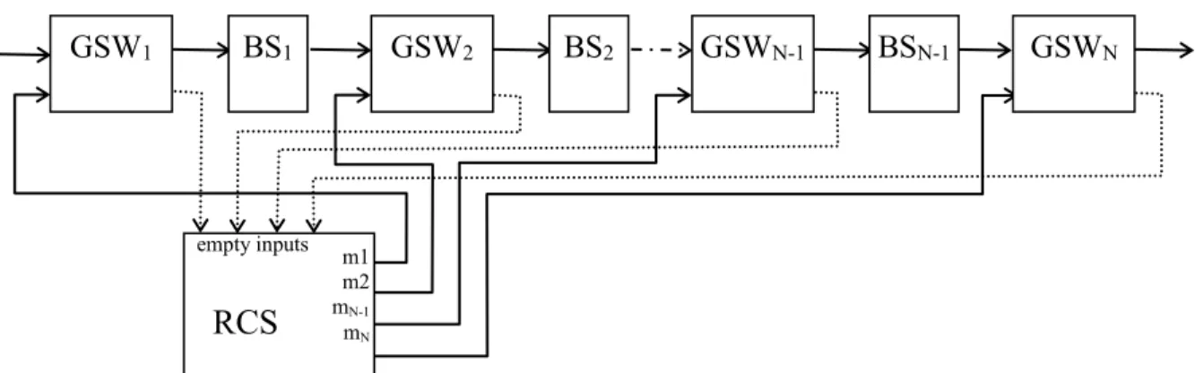
The simulation of this flow-shop is possible by developing two generic models via the
formalism DEVS: the Group of Sequential Workstations (GSWi) and the Buffer Stocks
(BSi). Next, by coupling these models, we obtain the complete flow-shop model which will
be simulated (refer to figure 7).
The simulation of the relocation requires a Removal Control System (RCS), which inhibits the various groups of machines operation during their removal.
The simulation technique retained is relatively simple. The line in its normal configuration was modeled according to an approach based on activities, each activity corresponding to a machine. All in all, about thirty activities were defined to simulate a production-type representing more than 80% of the cases of manufactured products.
In each case, the simulation starts one week before the beginning of the removal, in order to initialize the flow and to prepare the buffer stock, and ends one week after the end of the removal, once the stabilization of the flow has been achieved. The simulation of a removal stage (thus concerning a group) was obtained by the following mechanism:
for i=N to 1
Inhibition (mi=0) of new products entrance in the group of
workstations being moved (the creation of the upstream stock begins, while these machines empty gradually),
When the last Work-In-Process gets out of this group of machines (empty outputi =1), the time duration of its removal count down is started (tMov i),
At the end of this time, the inhibition of the entrance of products is suppressed (mi=1) and the products start to circulate again in the machine group that has just been moved,
Production by waiting for the next GSW removal.
next i.
Algorithm 2. Removal simulation algorithm.
Figure 7. Relocation flow-shop model. m1 m2 mN-1 mN RCS empty inputs GSW1 BS1 GSW2 BS2 GSWN-1 BSN-1 GSWN
5. SIMULATION OF A REMOVAL: AN INDUSTRIAL CASE
We present a removal project made necessary by the decrepitude of the initial site and a lack of available surface, due to the accumulation of new equipment over the years.
Having a new industrial building with more floor space allows a different organization of the machines, while keeping the same functional logic. This presents various advantages: better quality of life for the production staff, facilitated inventory control, and better brand image towards the clientele.
5.1. Presentation of the industrial study
This study was performed for a small sized company that produces printed circuit boards. Whereas the mass production of such products implies long production delays (several months), this firm produces small and medium sized series within 2 weeks, and even within 5 days in case of urgency. Its market is served by engineer to order manner. Each item to be manufactured is defined by the customer. Thus, each order needs to interpret the CAD requirements of the customer before manufacture can start: masks manufacturing, programming instructions of computer numerically controlled drill press…
Their requirement for responsiveness and continuous present on the market means that the removal must not interrupt the production, even temporarily.
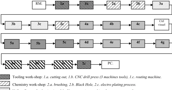
The production takes place on a production line composed of 24 workstations, automated or not, organized in 6 work-shops. Some workstations have several machines in parallel. Transfers between machines are principally manual, the integrated circuits being temporarily stored vertically on pallets where they are not in contact with one another. Some of these workshops are characterized by particular environmental conditions. Thus, in the chemistry and engraving workshops, where many foul-smelling effluents are emitted, extractions and air treatments must be performed regularly, while the place where photosensitive products are stored needs a polarized light and certain level of dust filtration. Figure 8 gives an idea of the sequence of production operations which allows the transformation of an epoxy plate covered with brass into two-sided PCBs.
The removal machine after machine is no longer adapted because the machines are too numerous and too heterogeneous. Some are simple to move whereas others need complex procedures. Therefore, we determined different possible machine groupings with specific removal characteristics: homogeneous removal times and small variations of the buffer stock volume.
5.2. Study of machine grouping strategies
5.2.1. Selecting the production line groups
The same production line can be moved machine after machine, or groups of machines after groups of machines. The choice of sequences of machine grouping must comply with technological rules and requirements. In fact, sometimes a product getting out of a certain machine must get into the following machine right away. For example, before the beginning of each of the engraving stages, a photosensitive layer is deposited on the epoxy plate by a first machine, then it is necessary to develop the layer immediately in an
exposure appliance and then another machine suppresses the non developed product: these three machines must not be moved separately, since they are part of a group.
This grouping for technological reasons may be needed in other instances, such as, in the food industry when there are shelf time constraints.
Tooling work-shop: 1.a. cutting out, 1.b. CNC drill press (3 machines tools), 1.c. routing machine. Chemistry work-shop: 2.a. brushing, 2.b. Black Hole, 2.c. electro plating process.
Yellow Room: 3.a.lamination, 3.b. film processing machine, 3.c. exposure appliance.
Engraving work-shop: 4.a. etching, 4.b. tin lead extraction bath, 4.c. washing machine, 4.d. furnace,
4.e. micrograving, 4.f. tinning, 4.g. washing machine.
Saving work-shop: 5.a. coating saving, 5.b. film processing machine, 5.c. exposure appliance. Silk Screen printing work-shop: 6.a. film processing machine, 6.b. exposure appliance, 6.c. paint.
Figure 8. The production line.
Furthermore, for the proposed method to operate properly, it is necessary to have a certain balance between the volumes of the successive stocks to be created. This imposes to create groups of machines with homogeneous removal times.
5.2.2. Application
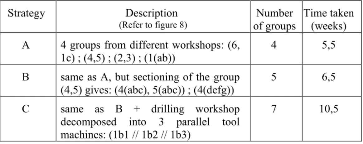
In our application, only a dozen strategies of segmentation have complied with the technological constraints. The smaller the buffer stock is, the more delicate the removal is. Therefore six segmentation strategies were studied. The segmentation by machine or by workshop proved inadequate. The best three solutions are shown in Table 1:
Solution A: grouping machines from different workshops.
Solution B: dividing different workshops so as to optimize the variations of the buffer stock. 4b 3b 3c 2c 4a 4c 5c 5b 4d 4e 4f 4g RM. 1a 1b 2a 2b 3a 6a 6b 6c 1c PC. 5a Ctrl visuel
Solution C: using the parallelism of the first drilling workshop and maintaining the production of some drilling machines during the removal of the other, to minimize the average buffer stock.
To test these solutions, an accurate simulation model of the production system and of its flow was necessary. It needed a ground inquiry to collect the exact specifications of the machines concerning their productivity and move ability.
Strategy Description (Refer to figure 8) Number of groups Time taken (weeks)
A 4 groups from different workshops: (6,
1c) ; (4,5) ; (2,3) ; (1(ab))
4 5,5
B same as A, but sectioning of the group
(4,5) gives: (4(abc), 5(abc)) ; (4(defg))
5 6,5
C same as B + drilling workshop
decomposed into 3 parallel tool machines: (1b1 // 1b2 // 1b3)
7 10,5
Table 1: Description of the proposed strategies A, B and C. 5.3. Exploring the simulation mechanisms
We describe the coupled DEVS modeled components announced in section 4.3 (figure 7). 5.3.1. The ‘GSW’ model description
In this section, we give an informal description of the behavior of ‘GSW’.
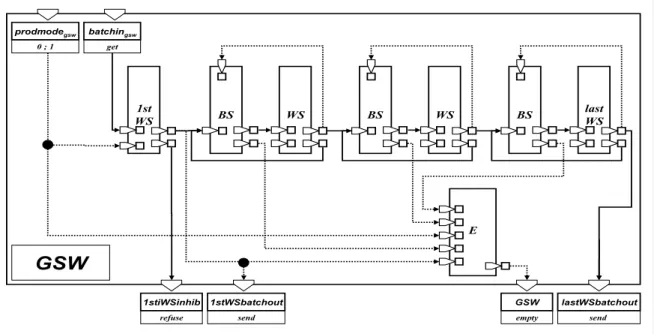
In a ‘GSW’ coupled model, several ‘WS’ models of workstations are associated in alternation with several ‘BS’ models of stocks. The goal is to obtain a ‘GSW’ model having globally an equivalent operation to that of a workstation ‘WS’ model. From the point of view of their external coupling, these two models have thus to be alike, even if
‘GSW’ model contains several ‘WS’ models. So a modular and hierarchical approach of
the production line modelling problem is obtained, which enables several configurations of the relocation. In figure 9, the case of a Group of Sequential Workstations (GSW) including 4 workstations is described. The principle is the same whatever the number n of buffer stocks and the number n+1 of workstations contained in the GSW is.
In this model, the problem consists in making sure that the whole of the group was really emptied before beginning the removal. For that, we must build a model which objective is to control the logical conditions indicating the empty states of each model component and to aggregate them. It is the goal of the sub-model 'E'.
5.3.2. The ‘E’ detailed model
The model 'E' is used to generate a logical signal indicating that a 'GSW' is totally empty of WIP: this implies it can be moved. The operations of model 'E' are activated when the model receives the order for the ‘stop during removal’ operating mode.
GSW 1st WS BS WS BS last WS BS WS 0 ; 1 prodmodegsw get batchingsw empty GSW lastWSbatchout send send 1stWSbatchout refuse 1stiWSinhib E
Figure 9. DEVS model of a group of sequential workstations (GSW) for relocation control.
b: formal description in DEVS
‘E’ = <XE, YE, S, ext, int, , t>
Input event variables: XE = (prodmodeE, capacity1, ..., capacityi, ...., capacityn,
capacityn+1), where:
‘prodmodeE’ = {0, 1} – this port gives the order for the operating mode of the
machine: the external event ?prodmodeE=’1’ indicates the normal production
operating mode, the external event ?prodmodeE=’0’ indicates the stop during
removal operating mode.
‘capacityi’ = {empty} for i=1,....,N,N+1 – this event indicates that the i-th element
is empty (for i=1,...,N it is a buffer stock, for i=N+1 is the first workstation),
State variables: S = {( phase,X , sigma)}, where:
Phase = {init, inhib, empty, verify, wait}, is a name representing the situation in the real world,
X is a vector of dimension N+1: each coordinate xi (i=1,...,N+1) of X
represent the empty state of the i-th element: the value '0' is the default value and it refers to the normal production operating mode, and the value '1' refers to the stop during moving operating mode and it signifies that the element is empty from parts,
sigma
0
IR , is the life time of the current state.
Output event variables: YE = (GSWE), where:
GSWE = {empty} – this event indicates that there are no more parts in the group of
The functions of the 'E' DEVS model are defined in the graph in figure 10: GSWE empty E ' ' ?capacityiempty ' ' !GSWEempty 1st BS of GSW empty capacity1 verify 0 1 i x wait infiniteX inhib infinite0 X empty 0I X if i:xi0 1 i x 1 , ,...., 1 i N N if ' ' ?capacityiempty generic BS of GWS last BS of GSW 0 ; 1 1stWS of GSW init infinite0 X ' ' ?capacityiempty ' 1 ' ?prodmodeE ' 0 ' ?prodmodeE empty capacityi empty capacityN empty capacityN+1 prodmodeE Figure 10. E model.
c: interpretation of DEVS model behavior
At the beginning, in the passive state 'init', characterized by a normal production, each
coordinate x of X is equal to 0 (X 0 ). Each event ?capacityi='empty' is ignored and the
first external transition is caused by the event ?prodmodeE='0'. The model reaches the
passive state 'inhib'. Each time an external event ?capacityi='empty' occurs, the i-th
coordinate of X changes its value from 0 to 1 and the model reaches the transition with
the state 'verify’. The internal transition which derives from this state depends on the
following condition: when xi=1, for each i=1,…, N+1, the transition is activated and a new
transitory state 'empty' is reached. The output signal !GSWE='empty' is produced when the
state 'inhib' is reached again. As long as there is still at least one i such as xi=0, the
transition ‘verify’ reaches a passive state 'wait' from which 'verify' can be reached again if a
new external event ?capacityi='empty' occurs.
When the model returns in 'inhib', it waits for the signal ?prodmodeE='1' to return to the
initial state 'init'.
5.3.3 The ‘GSW’ detailed coupled model
a: formal description in DEVS
‘GSW’ = <Xgsw, Ygsw, M, EIC, EOC, IC>
Input event variables: Xgsw = (batchingsw, prodmodegsw), where:
batchingsw = {get} – this event indicates the reception of a new batch by the group
of sequential workstation,
prodmodegsw = {0, 1} – this port gives the order for the operating mode of the
group: the external event ?prodmodegsw=’1’ indicates the normal production
operating mode (it is the default value), the external event ?prodmodegsw=’0’
indicates the stop during removal operating mode,