Multi-criteria and satisfaction oriented scheduling for hybrid distributed computing infrastructures

HAL Id: hal-01239218

https://hal.inria.fr/hal-01239218

Submitted on 7 Dec 2015

HAL is a multi-disciplinary open access archive for the deposit and dissemination of sci-entific research documents, whether they are pub-lished or not. The documents may come from

L’archive ouverte pluridisciplinaire HAL, est destinée au dépôt et à la diffusion de documents scientifiques de niveau recherche, publiés ou non, émanant des établissements d’enseignement et de

Multi-criteria and satisfaction oriented scheduling for

hybrid distributed computing infrastructures

Mircea Moca, Cristian Litan, Gheorghe Silaghi, Gilles Fedak

To cite this version:

Mircea Moca, Cristian Litan, Gheorghe Silaghi, Gilles Fedak. Multi-criteria and satisfaction oriented scheduling for hybrid distributed computing infrastructures. Future Generation Computer Systems, Elsevier, 2016, 55, �10.1016/j.future.2015.03.022�. �hal-01239218�

Multi-Criteria and Satisfaction Oriented Scheduling for

Hybrid Distributed Computing Infrastructures

Mircea Mocaa_{, Cristian Litan}a_{, Gheorghe Cosmin Silaghi}a_{, Gilles Fedak}b_,

a

Babes.-Bolyai University, Cluj-Napoca, Romˆania b_{INRIA, Universit´e de Lyon, France}

Abstract

Assembling and simultaneously using di↵erent types of distributed comput-ing infrastructures (DCI) like Grids and Clouds is an increascomput-ingly common situation. Because infrastructures are characterized by di↵erent attributes such as price, performance, trust, greenness, the task scheduling problem becomes more complex and challenging. In this paper we present the de-sign for a fault-tolerant and trust-aware scheduler, which allows to execute Bag-of-Tasks applications on elastic and hybrid DCI, following user-defined scheduling strategies. Our approach, named Promethee scheduler, combines a pull-based scheduler with multi-criteria Promethee decision making algo-rithm. Because multi-criteria scheduling leads to the multiplication of the possible scheduling strategies, we propose SOFT, a methodology that allows to find the optimal scheduling strategies given a set of application require-ments. The validation of this method is performed with a simulator that fully implements the Promethee scheduler and recreates an hybrid DCI environ-ment including Internet Desktop Grid, Cloud and Best E↵ort Grid based on real failure traces. A set of experiments shows that the Promethee scheduler is able to maximize user satisfaction expressed accordingly to three distinct criteria: price, expected completion time and trust, while maximizing the infrastructure useful employment from the resources owner point of view. Finally, we present an optimization which bounds the computation time of the Promethee algorithm, making realistic the possible integration of the scheduler to a wide range of resource management software.

Email address: mircea.moca@econ.ubbcluj.ro,

cristian.litan@econ.ubbcluj.ro, gheorghe.silaghi@econ.ubbcluj.ro, gilles.fedak@inria.fr(Gilles Fedak)

*Manuscript

Keywords:

Elastic computing infrastructures, Hybrid distributed computing

infrastructures, Pull-based scheduling, Multi-criteria scheduling, Promethee scheduling

1. Introduction

The requirements of distributed computing applications in terms of pro-cessing and storing capacities is continuously increasing, pushed by the gigan-tic deluge of large data volume to process. Nowadays, scientific communities and industrial companies can choose among a large variety of distributed computing infrastructures (DCI) to execute their applications. Examples of such infrastructures are Desktop Grids or Volunteer Computing systems [8] which can gather a huge number of volunteer PCs at almost no cost, Grids [12] which assemble large number of distributed clusters and more recently, clouds [4] which can be accessed remotely, following a pay-as-you-go pricing model. All these infrastructures have very di↵erent characteristics in terms of computing capacity, cost, reliability, consumed power efficiency and more. Hence, combining these infrastructures in such a way that meets users’ and applications’ requirements raises significant scheduling challenges.

The first challenge concerns the design of the resource management middleware which allows the assemblage of hybrid DCIs. The difficulty re-lies in the number of desirable high level features that the middleware has to provide in order to cope with: i) distributed infrastructures that have various usage paradigms (reservation, on-demand, queue), and ii) comput-ing resources that are heterogeneous, volatile, unreliable and sometimes not trustee. An architecture that has been proved to be efficient to gather hybrid and elastic infrastructures is the joint use of a pull-based scheduler with pilot jobs [37, 17, 35, 6]. The pull-based scheduler, often used in Desktop Grid com-puting systems [1, 10], relies on the principle that the comcom-puting resources pull tasks from a centralized scheduler. Pilot jobs consist in resource acquisi-tion by the Promethee scheduler and the deployment on them of agents with direct access to the central pull-based scheduler, so that Promethee can work with the resources directly, rather than going through local job schedulers. This approach exhibits several desirable properties, such as scalability, fault resilience, ease of deployment and ability to cope with elastic infrastructures, these being the reasons why the architecture of Promethee scheduler that we propose in this paper, follows this principle.

The second challenge is to design task scheduling that are capable of efficiently using hybrid DCIs, and in particular, that takes into account the di↵erences between the infrastructures. In particular, the drawback of a pull-scheduler is that it flattens the hybrid infrastructures and tends to consider all computing resources on an equal basis. Our earlier results [26, 27] proved that a multi-criteria scheduling method based on the Promethee decision model [11] can make a pull-based scheduler able to implement scheduling strategies aware of the computing resources characteristics. However, in this initial work, we tested the method on single infrastructure type at a time, without considering hybrid computing infrastructures, and we evaluated the method against two criteria: expected completion time (ECT) and usage price. In this paper, we propose the following extensions to the Promethee sched-uler: i) we add a third criteria called Expected Error Impact (EEI), that reflects the confidence that a host returns correct results, ii) we evaluate the Promethee scheduler on hybrid environments, iii) we leverage the tunability of the Promethee scheduler so that applications developers can empirically configure the scheduler to put more emphasize on criteria that are important from their own perspective.

The third challenge regards the design of a new scheduling approach that maximizes satisfaction of both users and resource owners. In general, end users request to run their tasks quicker and at the cheapest costs, op-posed to the infrastructure owners which need to capitalize their assets and minimize the operational costs. Thus, an overall scheduling approach should allow the resource owners to keep their business profitable and meantime, increase the end user satisfaction after the interaction with the global com-puting system.

The Promethee scheduler allows users to provide their own scheduling strategies in order to meet their applications requirements by configuring the relative importance of each criteria. However such configurable multi-criteria schedulers have two strong limitations: i) there is no guaranty that the user preferences expressed when configuring the scheduler actually translates in an execution that follows the favored criteria, and ii) the number of possible scheduling strategies explodes with the number of criteria and the number of application profiles, rapidly leading to an intractable situation by the user. We propose Satisfaction Oriented FilTering (SOFT), a new methodology that explores all the scheduling strategies provided by a Promethee multi-criteria scheduler to filter and select the most favorable ones according to the user execution profiles and the optimization of the infrastructure usage.

SOFT also allows to select a default scheduling strategy so that the scheduler attains a high and at the same time stable level of user satisfaction, regardless the diversity of user satisfaction profiles.

In this paper, we introduce the design of the fault-tolerant and trust-aware Promethee scheduler, which allows to execute Bag-of-Tasks applica-tions on elastic and hybrid DCI, following user-defined scheduling strategies. We thoroughly present the algorithms of the multi-criteria decision making and the SOFT methodology. Finally, we extensively evaluate the Promethee scheduler using a simulator that recreates a combination of hybrid, elastic and unreliable environment containing Internet Desktop Grid, public Cloud using Spot Instance and Best E↵ort Grid. Simulation results not only show the e↵ectiveness of the Promethee scheduler but also its ability to meet user application requirements. We also propose an optimized implementation of the Promethee algorithms and perform real world experiments to validate the approach.

The remainder of the paper is organized as follows. In section 2 we give the background for our work and define the key concepts, in section 3 we explain our scheduling approach and define the performance evaluation met-rics. In section 4 we define SOFT, the methodology for optimal scheduling strategies selection. Then we present the architecture of the implemented experimental system in section 5. In section 6 we describe the experimental data, the setup and present the obtained results and findings. In section 7 we discuss related work and finally section 8 gives the concluding remarks and observations on this work.

2. Background

This section describes the multi-criteria scheduling on hybrid DCIs prob-lem that we address in this work and defines the key concepts used in our discussion.

2.1. Description of the scheduling problem

In the considered context users submit their applications for execution on a system that aggregates the computing resources from at least three types of DCI: Internet Desktop Grids (IDG), Best E↵ort Grids (BEG) and Cloud. Each computing resource from the above mentioned infrastructures have di↵erent characteristics in terms of computing capacity, reliability, cost,

consumed power efficiency, and trust. For instance, Internet volunteer Desk-top PCs could be considered as free of charge but insecure and unreliable, while a Cloud resource can be costly but far more secure and reliable.

Users usually expect good execution performance but they are also con-cerned about other issues like cost, confidence and environmental footprint of the infrastructure. Thus, a relevant concern for task scheduling is to attain the best usage of the infrastructures in order to meet users’ expectations and, at the same time, insure a convenient capitalization of the resources for their owners.

2.2. Key concepts

Users submit bag of work-units to a centralized scheduler and expect (after a while) the corresponding results. For each work-unit the scheduler creates at least one task and inserts it into a BoT (Bag of Task). During the execution the scheduler aims at emptying this BoT by scheduling tasks to hosts belonging to various types of computing infrastructure.

We use a pull-based scheduling strategy. Hence our scheduler is a cen-tralized component (master) based on the pull communication model for the interaction with hosts (workers). The reason for this design choice is the requirement for elasticity and adaptability to structure disruptions that characterize DCIs like IDG and BEG. This model allows a complete inde-pendence of all system components [23]. The pull model allows workers to have the contact initiative, which overcomes the real issue of connecting to volunteers residing behind firewalls [20] or other security components.

When a host hih becomes available (either because it (re-)joins the

sys-tem or after completing a task) it contacts the scheduler in order to receive a new task. This approach is efficient [36] since in IDGs, hosts contact the server quite seldom. More, if embedded into a real middleware, such a scheduling component becomes more scalable, since it does not keep track of the workers’ state. Due to its advantages, many Desktop Grid systems (e.g BOINC[1], XtremWeb [10]), and Grid PilotJob framework (e.g FALKON [34], DIRAC[6]) and others rely on the pull model for the master-worker communication.

Due to the use of the pull model, the structure of the system and the scheduling process are driven by the behavior of participating hosts. As discussed above, there are two cases when a host pulls work: either when it (re-)joins the system, or after completing a task. We consider that a host may leave the system without preventing the scheduler. Such disruptions

may degrade the execution performance of a BoT and they are more likely to occur in IDG and BEG infrastructures.

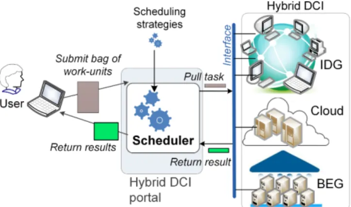
Figure 1 depicts an overview of the considered scheduling context. As our discussion is focused on the scheduling method, we omitted to detail additional middleware components and layers which naturally occur in real systems. For example, by Interf ace we designate specific mechanisms that allow hosts from di↵erent types of infrastructure to communicate with the scheduler. The details of this communication may di↵er from an infrastruc-ture type to another. For instance it may be directly from a host to scheduler in IDG or via a mediator component for Cloud, as used in [6]. However, such mechanisms do not fall within our research scope.

Figure 1: Overview on the Promethee scheduler architecture and its context.

Formalisms:

A work unit, denoted with wiw, represents a unit of work that must

be processed and for which an end user application expects a result from the scheduler. A work unit is characterized by:

– a unique identifier IDW_(w iw),

– the number of instructions NOI(wiw),

– the arrival time TMA(wiw). This is the time when the scheduler

received the work unit from a user application.

– the completion time TMC(wiw). This is the time when the

sched-uler completes a work unit by receiving a correct result for a cor-responding task.

A task tit is an instantiation tiw,r of the work unit wiw, r 2 N⇤. During

the execution, tiw,r is the r

th _{instance (replica) created for w}

iw, in the

aim of completing it. A task tit is characterized by:

– a unique identifier IDT_(t it),

– the number of instructions NOI(tit) (this value is inherited from

its corresponding work-unit),

– the creation time TC(tit). This is the time when the scheduler

created the task for an uncomplete work-unit, – the schedule time TMS(tit),

– the completion time TMC(tit).

A pulling host hih occasionally contacts the scheduler to pull a task

and is characterized by: – a unique identifier IDH_(h

ih),

– IDDCI_{, a label indicating the identity of the computing}

infrastruc-ture to which it belongs,

– the computing capacity CPU(hih), expressed in number of

pro-cessed instructions per second. For the sake of simplicity, in this work only CPU capacity is considered and not other types of re-source such as memory, bandwidth etc.

– PRICE(hih), which is the price (in monetary units) per second,

eventually charged by host for processing tasks.

After a host completes the execution of a task it contacts the scheduler to return the computed result and pull a new task.

A set of scheduling criteria C = {cic, 1 ic  Nc}, provided either by

the end user or by the infrastructure owner. For instance, a criterion cic

might be the expected completion time, the price charged for complet-ing a task on a particular infrastructure or the expected error impact. Each criterion cic will have assigned an importance weight !ic > 0, such

as P!ic = 1.

The scheduler holds a set of work units W = _{wiw, iw 2 N}, and a set

inserts into T a new task ts,r, r = 1, as previously explained. When a task

ts,r is scheduled, the scheduler inserts into T a new replica, ts,r+1. This r + 1

replica will have a lower priority for scheduling whilst the scheduler still waits to receive a result for the ts,r task.

3. The Promethee scheduling method

This section presents our approach of using Promethee[11] for task schedul-ing and the defined performance evaluation metrics.

3.1. The Promethee algorithm

When a host h pulls work, the scheduler uses the Promethee algorithm to rank the BoT based on the characteristics of the host. Then it selects the best ranked task and schedules it to the respective host.

Promethee[3] is a multi-criteria decision model based on pairwise com-parisons, which outputs a ranking of the tasks. This method considers a set of criteria C = {cic; ic 2 [1, Nc]} to characterize tasks and a set of

impor-tance weights for criteria, W = !ic(cic), so that

PNc

ic=1!ic(·) = 1. First, the

scheduler builds the matrix A = _{aic,it} where each element aic,it is computed

by evaluating task tit against criterion cic. For instance, if price=2 monetary

units/sec. and CPU=10 NOI/sec., the evaluation against this criterion for task t1 having NOI=100 is 20; similarly, for a task t2 with NOI=300 the evaluation

is 60. Matrix A is the input for the Promethee algorithm and characterizes the BoT for a particular pulling host.

Based on the input matrix A, for each criterion cic, the algorithm

com-putes a preference matrix Gic ={gi1t,i2t}. Each value gi1t,i2t shows the

prefer-ence P _{2 [0, 1] of task t}i1t over ti2t. This value is computed using a preference

function P that takes as input the actual deviation between the evaluations of ti1t and ti2t within each criterion cic. If the criterion is min/max and the

deviation is negative, the preference is 0/P (gi1t,i2t); it becomes P (gi1t,i2t)/0

when the deviation is positive. For short, the preference function brings the deviation value within the [0, 1] interval. Resuming the previous example, if the algorithm is configured with a min target for price, then t1 is preferred

to t2 with g1,2 = P (40); otherwise, if the target is set to max, g1,2 = 0 since

the price of t1 is smaller than that of t2.

For each criterion, the algorithm continues with the computation of +_,

which shows the power of a task to outrank all other tasks j. The computa-tion aggregates gi1t,j values (summation per line in matrix G). In a similar

way, is computed to express the weakness of a task while being outranked by all other tasks j. The computation aggregates gj,i1t values (summation per

column) in matrix G. For each criterion, a net flow is computed as + .

Figure 2 depicts the calculation of the positive flow + _{- summation by line}

of the preferences and for the negative flow - summation by column, for the t0 task.

Figure 2: Computing positive and negative outranking flows for task t0.

Finally the algorithm calculates an aggregated flow as a weighted sum on the net flows, using the importance weights ! assigned to criteria. This final aggregated flow is a list of scores for each task in the BoT. The task with the highest score is scheduled to the pulling host.

We notice that the Promethee algorithm uses a preference function P to calculate a preference among two tasks. The literature [11] suggests several definitions for the preference function, including Linear, Level, Gaussian and others. However, one is free to provide any other definition for this function. In section 6.3.2 we show how to choose an efficient preference function. 3.2. Evaluating tasks against a set of scheduling criteria

Before making a scheduling decision, the scheduler creates the evaluation matrix A, as previously described, by evaluating all tasks against each crite-rion in the considered set _{C. In this section we describe the policies for} eval-uating tasks for a set of three criteria: the expected completion time, price and expected error impact. Although in our work we used three scheduling criteria, one can easily define and add her own new criteria to this scheduling method.

The Expected Completion Time (ECT) represents an estimation of the time interval needed by a pulling host to complete a particular task. This is calculated by dividing the number of instructions (NOI) of a task by the computing capacity (CPU) of the host.

The Price represents the estimated cost (expressed in monetary units) eventually charged by the pulling host for the completion of a task. This is computed as a product between the ECT and the price/time unit required by host. In our scheduler, if a host returns the result of a task later than its ECT the total cost for the execution of the BoT remains unchanged. By this approach we seek to mimic what happens in a real system where the SLA1

can include agreed execution time limits and penalties if exceeded.

The Expected Error Impact (EEI) indicates the estimated impact of scheduling a particular task to the pulling host taking into account its repu-tation (error proneness) and the size of the task. For a less trusted pulling host the evaluation of a larger task would result into a higher error impact. The idea of using this criterion is to mitigate the behavior of scheduling large tasks to mistrusted hosts. In algorithm 1 we give the calculation steps for the EEI(ti) evaluation.

In order to create a realistic behavior of the hybrid DCI, in our experi-mental system we consider that hosts can produce erroneous results or even fail to return a result to the scheduler. In real systems this is either due to hardware/platform issues or due to malicious behavior of the hosts (i.e. in BOINC). Hence we use two parameters to model this behavior in each type of infrastructure: f the fraction of hosts that produce erroneous results and s, the probability with which they manifest this behavior. In order to use this information within the scheduling method we implemented a simple reputa-tion model like the one described by Arenas et al. in [2]. The idea is that the scheduler computes and keeps track of hosts’ reputation, based on the quality of the returned results during the execution. We assume that the scheduler has a result verification mechanism to check the validity of the results re-ceived from hosts. According to the implemented model, if a host returns an erroneous result for a large task, its reputation will be more severely a↵ected compared to the erroneous result of a small task. Besides, the reputation score is more significantly a↵ected by the quality of the soonest completions.

With respect to this rule, our scheduler computes a host’s reputation based on a maximum of 5 last returned results. By this, the scheduler takes into account the recent behavior of hosts within the system.

Algorithm 1 The calculation of EEI(ti)

1: Calculate the reputation of the pulling host, Rhih_.

2: Calculate the relative utility ⌥(ti) = _{N OI}N OI(t_maxi) {The utility of task tirelative to its size}.

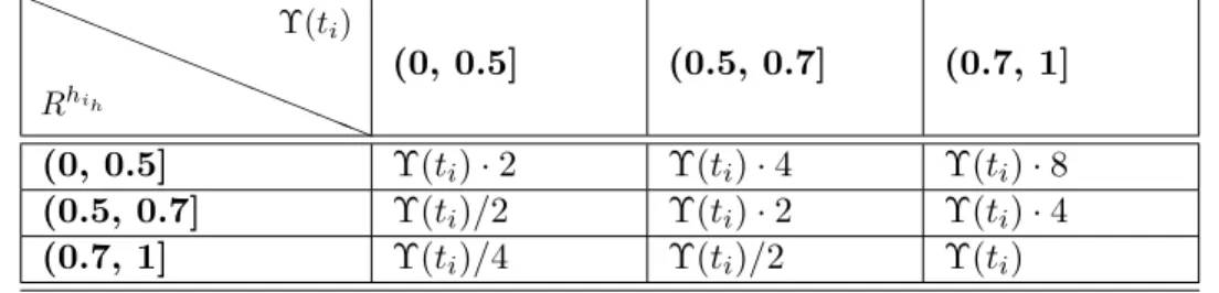
3: Based on Rhih _{and ⌥(ti) calculate EEI(ti) using a policy, like in table 1.}

aa_aa aa_aa aaa Rh_ih ⌥(ti) (0, 0.5] (0.5, 0.7] (0.7, 1] (0, 0.5] ⌥(ti)· 2 ⌥(ti)· 4 ⌥(ti)· 8 (0.5, 0.7] ⌥(ti)/2 ⌥(ti)· 2 ⌥(ti)· 4 (0.7, 1] ⌥(ti)/4 ⌥(ti)/2 ⌥(ti)

Table 1: EEI calculation scheme.

In table 1 we describe the EEI calculation scheme used in our implemen-tation. This can be seen as a risk matrix, where EEI indicates the risk of scheduling a task of a certain size to a host with a particular reputation. The values in the table show that:

the higher the relative task utility, the bigger the EEI value (for a particular reputation score) and

the higher the host reputation, the smaller the EEI value (for a partic-ular task relative utility).

3.3. Performance evaluation metrics

To evaluate the performance of the scheduling approach we use the fol-lowing metrics: makespan, cost, execution efficiency, the user satisfaction ⇥ and the infrastructure utilization efficiency

"

.

We define makespan (M ) like Maheswaran et al. in [24], as the duration in time needed for the system to complete the execution of all work units belonging to the same application execution. This is computed by scheduler as the di↵erence between the timestamp of the result received for the last

uncompleted task and the timestamp of the first task schedule. In all ex-periments the makespan reflects the execution at hosts plus the scheduling decision making time but not the network communication between scheduler and hosts. We consider that this value has no relevance for the evaluation of the scheduling method in the scheduling context defined in section 2.2.

The cost (C) indicates the total cost in monetary units accumulated for an entire application execution. Each result returned by a host to scheduler may increase the total cost of the whole execution. Exceptions from the cost cumulation are when a host returns the result after the estimated completion time. In a real system, this situation could be when a host from a Cloud infrastructure violates the SLA agreement.

The execution efficiency (E) is calculated for an application execution as a ratio between the number of instructions from successfully executed tasks and the number of instructions from the total scheduled tasks. Hosts that are error prone or those who fail, lead to a smaller execution efficiency since the tasks they received must be rescheduled.

In order to facilitate the analysis of the scheduling performance we add up the metrics defined from user perspective into the aggregated objective function ⇥. This indicates the overall user satisfaction and it is defined in eq. 1. Given that, based on a set of parameters, a system designer can configure the scheduler in di↵erent ways using a set of strategies S, ⇥ shows the relative satisfaction perceived by user Uiu after the completion of her

application, for a specific strategy s from S. For instance, a high m and a

low c shows that the user is more satisfied by a faster but costly execution,

while a low m and a high c indicate that the user is more satisfied by a

slower but cheaper execution of their application.

⇥Uiu s (M, C, E) = m· Mmax MUviu Mmax Mmin + c· Cmax CvUiu Cmax Cmin + e· (1 Emax E Uiu v Emax Emin ) (1) where

Mmax, Cmax, Emax(and Mmin, Cmin, Emin) represent the maximum (and

minimum) values of makespan, cost and execution efficiency measured for the BoT execution in all strategies within _S.

m, c and e denote weights of importance from the user perspective

Uiu over makespan, cost and execution efficiency. After the completion

of their applications, end-users can compute the perceived satisfaction in their own ways. For this we define the set of unique user satisfaction profiles L = {lil, lil = ( m, c, e)} where m, c, e 0 and m + c+

e = 1.

From the resource owners’ perspective we measure the relative infras-tructure utilization efficiency

"

, defined in eq. 2.

"

DCI_iDCI s = N OIutil s (DCIiDCI) N OItot s (DCIiDCI) (2) where, for a given strategy s from the set S1 (defined in section 4.2):

N OItot

s (DCIiDCI) denotes the total number of operations executed on a

particular infrastructure DCIiDCI during the execution of a workload.

N OIutil

s (DCIiDCI) denotes only the number of operations executed on

a particular infrastructure DCIiDCI that led to work-units completion.

Obviously, N OItot(DCIiDCI) N OIutil(DCIiDCI) since hosts can fail before

completing tasks, the computations can last longer than the expected com-pletion time or the scheduler simply drops the erroneous results and schedule new replicas of the respective tasks.

We consider that the greater the relative efficiency of the resource utiliza-tion, the bigger the satisfaction of their owners.

4. Overall scheduling approach

This section presents our contribution in defining a methodology that allows one to select from a large number of defined scheduling strategies the optimal ones with regard to a set of application requirements.

4.1. The SOFT Methodology

In this section we give the Satisfaction Oriented FilTering (SOFT) method-ology. This allows one to select the optimal scheduling strategies given her own set of criteria _{C. Its essence derives from the practice of the performed}

Algorithm 2 SOFT methodology for optimal scheduling strate-gies selection.

1: Let cic be a criterion fromC, the considered set of criteria.

2: for all cic 2 C do

3: Define the evaluation of a task ti within this criterion {used for building the evaluation matrix A, as discussed in section 3}.

4: Define an appropriate metric and integrate it into the aggregating metric ⇥ {the definition proposed in section 3.3 can be extended}.

5: end for

6: Define _{S, a set of scheduling strategies based on: the criteria set C, min/max} target for each criterion and combinations of importance weights assigned to criteria {as in table 7 and 8}.

7: Define L, a set of user satisfaction profiles _{as in table 9}.

8: for all strategy s in S do

9: Run the system to complete a workload and record values for metrics defined at step 4.

10: end for

11: for all profile l in L do

12: for all strategy s in_{S do}

13: Calculate ⇥s.

14: end for

15: end for

16: From _{S extract a subset S}1 by applying a filtering method {we proposed Filter1 with Winabs_/Winfreq_{selection methods in section 4.2}.}

17: Define an efficiency metric

"

from the resource owners perspective. _{we proposed

"in section 3.3}

18: From S1 extract a subset S2 by applying a filtering method that employs

"

{we proposed Filter2 in section 4.2}.

experiments and analyses. So we describe a detailed process, from the def-inition of new criteria to the selection of a particular set of strategies that are optimal from both user and resource owners perspectives. Algorithm 2 defines the proposed methodology.

The methodology begins with the definition of criteria to be integrated into the scheduler and a corresponding metric for each (steps 1-5). On the constructed set of possible scheduling strategies (step 6) a selection method is applied in order to find those that provide high and stable user satisfaction levels (steps 7-16). On this resulting subset a second selection method is

applied in order to retain the strategies that are also the most efficient from the resource owners perspective (steps 17-18).

4.2. Finding optimal scheduling strategies

When using this scheduling method into a real system, its designer can configure the method through several key parameters which impact on the defined metrics. For instance, one may define a large variety of scheduling strategies by:

1. setting either max or min target to the task evaluation criteria pre-sented in section 3.2, and

2. by defining di↵erent combinations of importance weights !, assigned to those criteria.

To address this challenge, in this section we propose a methodology that supports a scheduler designer in finding optimal scheduling strategies given the formulated conditions. Our methodology is generic and independent from the number and type of considered scheduling criteria. Conse-quently, the advantage is that one can use it to configure the scheduler for her own set of criteria.

The methodology yields a set of optimal strategies considering all defined user satisfaction profiles at a time, but it can also be applied (with small adaptation) in a similar way for a particular profile only.

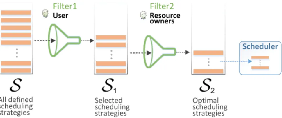
Figure 3 depicts the method, which at the highest level consists of two phases: Filter1 - defined from the users’ perspective and Filter2 - defined from the resource owners perspective. From the set of all defined scheduling strategiesS, Filter1 selects the strategies that conveniently satisfy the users, resulting S1. Next, Filter2 selects from S1 the strategies that satisfy the

resource owners (i.e. increasing the capitalization of their infrastructures) resulting S2. Finally, a scheduler designer can use the strategies from S2 to

configure the scheduler.

From section 2.2 recall Nc, the number of scheduling criteria in the

com-plete set of considered criteria C and !ic the importance weight assigned to

a criterion cic. Based on C and the min/max target assigned to each

cri-terion there are a number of 2Nc _{possible families of scheduling strategies.}

Moreover, for each family i 2 {1, ..., 2Nc}, one may assign values for the

weights !1, !2, ...!Nc such that

PNc

j=1!j = 1, !j 2 [0, 1) in di↵erent

combi-nations. Therefore, a scheduler designer faces the problem of optimizing the scheduling method on these two key parameters.

Figure 3: Method for selecting optimal scheduling strategies from user and resource owners perspectives.

Based on the optimization parameters we define a scheduling strategy s as a tuple ((b1, . . . , bi, . . . , bNc), (!1, !2, ..., !Nc)), with bi 2 {0, 1}, where

0/1 stands for min/max. Thus, the set _{S can be split into 2}Nc _strategy

families.

In the following we define the Filter1 and Filter2 phases. First, for each strategy s _{2 S and a sample L of N}L user profiles over L we compute the

⇥ metric and obtain a satisfaction sampling distribution characterized by the sample mean ¯us = _N1_L

NL

P

l=1

⇥l and the sample standard deviation s =

s 1 NL 1 NL P l=1 (⇥s u¯s)2.

Filter1 works in two steps:

Step1 constructs the set _S0 _{from strategies s that achieve both:}

X a corresponding user satisfaction distribution of user satisfaction values so that ¯us

s is above some chosen percentile q1, when sequentially

considering all the u¯s

s distributions of values restricted to each strategy

family and

X a flat positive satisfaction for all users, i.e. s = 0 and ¯us > 0.

Step2 further selects from _S0 _{a set of strategies S}

1, by applying one of

Absolute winners (Winabs_):

Select the strategies that obtain the largest p values (e.g. p = 2) in the descending order of ¯us.

Frequency winners (Winfreq_):

Based on the distribution of ¯us values, select the strategies s 2 S0

so that ¯us is above some percentile q2. Among these, identify those

strategy families i which appear with the highest p frequencies (e.g. p = 2). Then, select the strategies that belong to the identified families and also for which weights !(.) occur with the highest frequency in the

initially selected set of strategies.

Step1 provides a primary filtering of all strategies in S, by selecting the ones that are among the first (i.e. fall into the q1 percentile) in terms of

average satisfaction value per unit of risk. The risk is represented by the heterogeneity of the considered user profiles, L. After this step we obtain the most homogeneous strategies with respect to the induced benefits. Step2 proposes two methods for further refining the strategies set: either Winabs

which trivially selects the strategy with the highest mean utility value, or Winfreq _{which takes into account the stochastic nature of user satisfaction}

realizations.

Filter2

From the_S1 set, this phase further selects the strategies that perform well

from the resource owners perspective. Hence, for each s _{2 S}1 we compute

the infrastructure utilization efficiency ✏ for each considered infrastructure DCIiDCI. Thus for Ndci infrastructures, we obtain a distribution of values

{✏(k)s , k = 1, ..., Ndci} with mean ¯✏s = _N1_dci NPdci

k=1

✏(k)s , representing the average

infrastructure utilization efficiency of strategy s. Given these, we finally select the strategies s so that ¯✏sis above a percentile q3within the distribution

of the obtained values. These strategies form the S2 set which is further

embedded into the scheduler.

In section 6.3.5 we present the results of applying this methodology for a setup with 3 scheduling criteria, 10 user satisfaction profiles (given in table 9) and 8·28=224 scheduling strategies.

5. Scheduling method implementation

In this section we describe the architecture of the scheduler implemen-tation and other complementary components. The scheduler in general is inspired from the XtremWeb behavior, borrowing basic functional compo-nents like the pull-based and task replication mechanisms.

Figure 4 depicts a component-based representation of the implemented system architecture; its main components are: the Task Scheduler, the trace-based Hybrid DCI Simulator and the Visualizer.

Figure 4: Experimental system architecture.

The Task Scheduler is a real implementation of the proposed scheduling approach. This component is responsible for selecting and scheduling tasks to pulling hosts. This component is called by the EvCtrl component when consuming a HJ (host join) or RET (return result) event from the queue. The e↵ective decision making for the task selection is delegated to the SDM component, which, at its root implements the Promethee decision model, described in section 3.

The Hybrid DCI Simulator realistically reproduces the behavior of hosts from di↵erent types of computing infrastructure. It is based on events created from real failure traces. In this way we obtain hybrid IN/OUT behavior of

hosts originating from di↵erent types of DCI. After reading the experiment configuration, the TraceLdr component can load di↵erent subsets of hosts from any combination of DCIs and for particular time-windows from the total available trace-period. For each DCI type, the DCIFactory creates hosts accordingly in terms of CPU, price, error rate and energy efficiency. Before running an experiment, all hybrid DCI infrastructure events (HJ and HLE(host leave)) are created and added to the EvPQ. Also, based on workload information for each user, the EvFactory creates and adds WKUA (work unit arrival) events to the EvPQ queue.

The EvCtrl is the main component of the simulator, controlling the com-pletion of BoTs. For this, after the creation of the hybrid DCI and workload, EvCtrl starts the execution of the workload by consuming events from EvPQ in a priority order, given by a time-stamp.

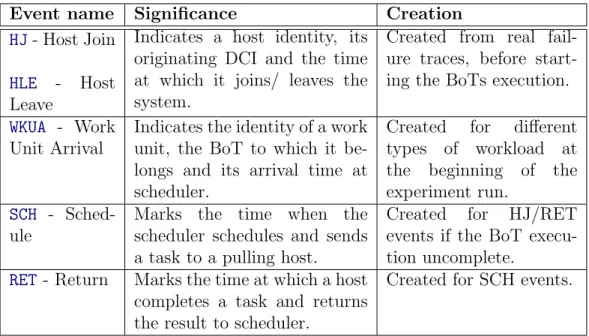
During the execution, based on the type of event currently being con-sumed the simulator creates new events, which we describe in table 2.

Event name Significance Creation

HJ- Host Join Indicates a host identity, its originating DCI and the time at which it joins/ leaves the system.

Created from real fail-ure traces, before start-ing the BoTs execution.

HLE - Host Leave

WKUA - Work

Unit Arrival

Indicates the identity of a work unit, the BoT to which it be-longs and its arrival time at scheduler.

Created for di↵erent

types of workload at the beginning of the experiment run.

SCH -

Sched-ule

Marks the time when the scheduler schedules and sends a task to a pulling host.

Created for HJ/RET

events if the BoT execu-tion uncomplete.

RET- Return Marks the time at which a host completes a task and returns the result to scheduler.

Created for SCH events.

Table 2: Rules for creating new events by the experimental system.

Algorithm 3 shows the order in which EvCtrl component consumes events. EvCtrl component reads events from EvQueue in their priority or-der. For some of them, new events are created or existent ones are deleted from the queue. For instance, when a host leaves during the execution of a

Algorithm 3 The event processing algorithm.

1: e = next event in EvQueue 2: if type of e is HJ then

3: Call the SDM component to select a task tit and schedule it to the

pulling host.

4: else

5: if type of e is HLE then

6: for all event 2 EvQueue do

7: if type of event is not HJ or HLE then

8: remove event from EvQueue

9: end if

10: end for

11: end if

12: else

13: if type of e is WKUA then

14: wiw = the received work unit

15: Create task tiw,1

16: Add tiw,1 to T

17: end if

18: end if

task, the return result event (HLE) associated to the fallen node is deleted. Consequently, the scheduler will not receive the result for the respective task, causing a rescheduling of a new replica of the task.

During the execution of the system, the EvCtrl component calls the Stats component to log relevant meta-information about the tasks’ comple-tion process. We use this output for the characterizacomple-tion of the experimental data in section 6.1 and to retrieve efficiency metrics of the infrastructures’ utilization in section 6.3.6.

The Visualizer creates custom representations of the meta-information collected by the Stats component during the system execution. Figure 4 was drawn from the information produced by the Visualizer. This facilitates the understanding of the di↵erent behaviors of the infrastructures in terms of availability of the hosts. The output of the Visualizer proved to be useful for driving our investigations, helping us to better understand the distribution of the tasks on di↵erent types of DCI.

6. Experiments and results

This section presents the experimental setup used for the validation of the scheduling approach presented in the previous sections. More precisely, we showed how to apply the scheduling methodology devised in section 4.2, in order to select the proper tuning of the scheduler, considering a hybrid computing infrastructure. We start by presenting the experimental data and setup then we discuss the obtained results.

6.1. Experimental data

With the aim of observing the behavior and measuring the performance of the proposed scheduling method, we developed and ran the system presented in section 5. The considered hybrid computing infrastructure was created by loading real failure traces [21, 19] as found in the public FTA (Failure Trace Archive) repository [15] for three types of infrastructure:

IDG: For Internet Desktop Grid, the system loads BOINC failure traces (from the SETI@home project) characterized by highly volatile resources. The traces contain 691 hosts during a period of 18 months, starting from 2010.

Cloud: For this environment the simulator loads Amazon EC2 spot instance traces containing 1754 hosts from 2011. Observing the traces, the resources are very stable.

BEG: The Best E↵ort Grid is an infrastructure or a particular usage of an existing infrastructure (like OAR [5]) that provides unused com-puting resources without any guarantees that these remain available to user during the complete execution of his application [9]. For the creation of this environment, the simulator loads Grid5000 traces with host join and leave events for a period of 12 months (during 2011) from the following sites: Bordeaux, Grenoble, Lille and Lyon. The traces capture the activity of 2256 hosts. Inspecting the files we observe that the resources are quite stable, meaning that small groups of machines go o↵ approximately at once for a small number of hours.

When the experimental system loads the failure traces, it assigns CPU capacity and price values to each host, according to the type of the origi-nating DCI. The values are randomly chosen with uniform distribution from the ranges given in table 3. As order of magnitude, the values were set

DCI type

CPU capacity

(number of executed instructions/ sec-ond)

Price charged by host

(monetary units/

sec-ond) IDG {50, 100, 150, 200, 250, 300, 350, 400} 0 Cloud 250 0.001 300 0.005 350 0.0075 400 0.01 BEG _{{50, 100, 150}} 0

Table 3: Host CPU capacity and price values for the considered types of DCI.

so that a host having the maximum considered CPU capacity completes the largest task (107_{instructions) in almost 7 hours and the smallest task}

(106_{instructions) in 40 minutes. While hosts from IDG and BEG compute}

for free (0 price), the hosts from Cloud require a price for their computa-tions. The values in table 3 show that more powerful Cloud hosts are more expensive. In all experiments, CPU capacity and price are constant for a particular host throughout the execution of the BoT. Therefore we do not consider dynamic pricing models.

In real systems, hosts originating from di↵erent infrastructure types man-ifest unequal reliability levels. To mimic this aspect in our experiments we created three types of host behavior concerning the moment in time when a host returns the result for a completed task, relative to the estimated ECT (at scheduler):

In time - when a host returns the result for a particular task at the expected completion time.

Delay - when a host in order to complete and return the result for a task needs more than ECT. For this behavior, 15% of the results from a BoT are delayed with a factor between (1, 1.5].

Never - when a host do not yield the result for a particular task. For this behavior we consider that for 5% of the BoT, hosts never send a result to the scheduler. This is di↵erent from a host leaving the system (according to the failure traces). In that case, the same host may rejoin the system and pull for work again, while in this behavior the host is available, but do not finish the computation (due to a local error).

In all experiments we use all three behaviors, except the experiment from section 6.3.1, where we distinctly analyze the scheduler performance on each particular type of behavior.

From the publicly available failure traces we randomly selected subsets of hosts so that the aggregated CPU capacity per type of DCI is roughly equal. By this approach we obtain three types of computing infrastructure, which are comparable. They are balanced in terms of total computational capacity while having di↵erent degrees of heterogeneity in terms of availability, price and error-proneness.

For our purpose we kept static the individual characteristics of hosts for the duration of the experiments. It is out of the scope of this paper to investigate our scheduling approach with dynamic host models, like dynamic pricing of the computation.

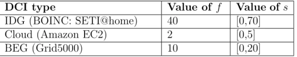
In section 3.2 we shortly described our approach of considering two pa-rameters f and s to implement the error proneness behavior of some hosts within the computing infrastructures. Recall f , the fraction of hosts that produce erroneous results and s, the probability with which they manifest this behavior. Our scheduler implements a simple reputation model[2] and computes the reputation of the pulling host, before the task evaluation phase (described in section 3.2). During the task evaluation phase, the scheduler uses this reputation score to calculate the expected error impact (the EEI criterion described in section 3.2). In our experiments we consider the f and s parameters as in table 4 - all values are expressed in % and have uniform distribution:

DCI type Value of f Value of s

IDG (BOINC: SETI@home) 40 [0,70]

Cloud (Amazon EC2) 2 [0,5]

BEG (Grid5000) 10 [0,20]

Table 4: Values for the f and s parameters.

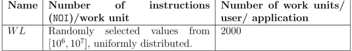
Table 5 describes the workload for one user and one application execu-tion.

6.2. Experimental setup

Each experiment is performed according to a particular setup, which is defined by a set of key parameters. For one setup, the value of a target

Name Number of instructions (NOI)/work unit

Number of work units/ user/ application

W L Randomly selected values from

[106_{, 10}7_{], uniformly distributed.}

2000

Table 5: Description of the scheduler workload.

parameter may vary on a defined range and the other parameters take fixed values. This basic approach allows us to study the impact of the target parameter on the tracked metrics. For comparability, we used the same workload (presented in table 5) into the experimental system, for various particular setups.

For each experiment run, the system performs the following steps, in the given order:

1. Read the experiment setup from a configuration file.

2. Create the hybrid DCI by loading failure traces and instantiating HJ and HLE events for each type of DCI. In all experiments we use a hybrid DCI composed from Cloud, IDG and BEG, unless otherwise specified. 3. Create the workload for all users by instantiating the WKUA event. 4. Start the execution of the workload on the hybrid infrastructure. The

running of an experiment ends when all work units within the given workload are complete.

5. Report the obtained results. 6.3. Results

This section presents the results of the experiments driven for the valida-tion of the proposed multi-criteria scheduling method. The evaluavalida-tion begins with simple scenarios focused on the specific mechanisms of the scheduling method. Next we propose a set of optimizations for the scheduler and show how to find optimal scheduling strategies by applying the filtering method defined in section 4.2.

6.3.1. Primary performance evaluation

In this section we validate the performance of the task scheduling method by comparing it with the First-come-first-serve (FCFS) approach, using makespan and cost as metrics.

The FCFS (F irst Come F irst Served) method assumes that the scheduler randomly selects a task and assigns it to a pulling host.

Experimental setup: For each method, combination of DCIs and type of host behavior we measure and report the makespan for the completion of the workload.

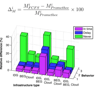
In order to obtain a clear performance overview between the proposed scheduling method and FCFS, we depict the relative di↵erence of makespan in figure 5. The values are calculated using eq. 3.

i M = Mi F CF S MP rometheei Mi P romethee ⇥ 100 (3) 1 2 3 IDG BEG_Cloud

0 10 20 30 40 Behavior Relative difference (%) In time Delay Never IDG, Cloud IDG, BEG BEG,

CloudIDG, _{BEG, Cloud} Infrastructure type

Figure 5: Performance improvement of the proposed scheduling approach and FCFS.

We observe that the Promethee-based scheduling outperforms FCFS, at di↵erent degrees in the considered types of DCI. While in Cloud environment the di↵erence is 9-12%, a better performance (32% improvement) of the proposed scheduling method is shown for IDG, for the never behavior. Also, the proposed scheduling method shows a 38% improvement for the IDG-BEG hybrid infrastructure. As a general remark, our scheduling method performs significantly better on infrastructure combinations containing IDG (in which hosts are more likely to fail).

6.3.2. Evaluating Promethee scheduler overhead

When designing the scheduler, one can choose from several preference functions. These functions have di↵erent complexities and though di↵erent real execution costs (in terms of CPU cycles), on the machine running the

scheduler. In this section we evaluate the overhead of the scheduler for the following preference functions:

PLinear(dic) = ⇢ _dic if dic  1 otherwise PLevel(dic) = 8 < : 0 if dic < q 1 2 if q dic < p 1 if dic p PGaussian(dic) = ( 1 e dic 2 2 2 if d_i c > 0 0 otherwise where:

dic is the deviation between the evaluations of two tasks within a

cri-terion cic: dic(t1, t2) = aic,1 aic,2;

is the standard deviation of the di↵erences dic for all pairs of tasks;

q is the degree of indi↵erence; any deviation below q leads to considering t1 and t2 equivalent;

p is the degree of preference; any deviation greater than q gives a strict preference, either 0.5 (for deviations between q and p) or 1.

Experimental setup: for each type of considered preference functions (Linear, Level and Gaussian) we run the system to complete the same W L workload.

Figure 6 presents real execution time measurements of the decision-making algorithm, implemented by the SDM component (presented in section 5). While the values on the y axis represent duration in milliseconds for each scheduling decision making, the x axis shows the scheduling iterations needed for a workload completion. The results regard the Linear, Level and Gaussian preference functions. The graph clearly shows that Gaussian is significantly more CPU-consuming, compared to the Linear and Level functions. Conse-quently, although the Linear and Gaussian functions yield similar makespan values (as mentioned in section 6.3.3), when designing a real system one should use the Linear function due to its execution cost efficiency. In this chart, the execution time needed for making a scheduling decision decreases with the completion process, since the decision is computed on smaller sets of tasks.

100 101 102 103 0 100 200 300 400 500

Scheduling iterations for the completion of a workload.

Real execution time (ms.)

Level Gaussian Linear

Figure 6: Real execution time values for the SDM component during the completion of a W L workload.

6.3.3. Tuning the scheduling method to increase performance

From section 3.1 we recall the preference function P , which may impact on the performance of the task selection algorithm. Therefore in this experiment we studied the achievements of the scheduler in terms of makespan when using the Linear, Level preference functions compared to FCFS. We also analyzed the consistency of the attained performance with respect to the utilized failure traces.

Experimental setup: in this experiment, for each method (Linear, Level, Gaussian and FCFS) the system is run 120 times to complete the same workload. For all methods the completion is carried by the scheduler with the same set of hosts but loading the failure traces at di↵erent start-points in time. By this we aim at proving that the relative performance of the proposed scheduling method is consistent with respect to the host failure behavior in time. In this experiment we use a hybrid DCI, composed from IDG, Cloud and BEG. First we compare our scheduler using Level and Linear preference functions described in section 6.3.3 and a FCFS scheduler. Table 6 presents the descriptive statistics regarding the makespan distri-bution for the considered setup.

Figure 7 depicts the empirical cumulative distribution functions (CDFs)

2_{P-values are computed for the Kolmogorov-Smirnov test of normality under the null} hypothesis is that the distribution of makespan is Gaussian.

Method Mean (STDEV) Di↵erence (%) The p-values2 Linear 367540,26 (104523,14) 0 0,190 (> 10%) Gaussian 371987,49 (105017,32) +1,21 0,214 (> 10%) Level 414840,79 (110604,18) +12,86 0,466 (> 10%) FCFS 432419,97 (118178,69) +17,65 0,831 (> 10%)

Table 6: Descriptive statistics of the makespan distributions for each method.

1 2 3 4 5 6 7 x 105 0 0.2 0.4 0.6 0.8 1 Makespan Probability Linear FCFS Level

Figure 7: Stochastic dominance of the Linear method with respect to the F CF S and Level methods.

of the execution times for the three methods. The Y-axis depicts the values of the CDF function F (M ) of the makespan M , showing the probability that the makespan records values lower than the scalar on the abscissa. We observe that the Linear function strictly dominates the other two methods, in the sense that FLinear > FLevel and FLinear > FF CF S for all values on

the abscissa. We also tested the dominance of the Linear method over the Level and F CF S using the t test for the equality of means in two samples and the Levene’s test for equality of variances in two samples with 99% confidence level, and the results are the same. Statistical tests show a weak dominance of Level over F CF S, therefore we conclude that the designed scheduling method based on the Promethee decision model is superior to F CF S. We omitted the representation for the Gaussian function because its performance is very similar to the Linear function and they overlap.

6.3.4. Adjusting the Promethee window size

As stated in section 2.2, the scheduler makes a new scheduling decision for each pulling host. Hence, each time, the whole BoT is given to Promethee as input.

In this experiment we are interested in finding out whether for a par-ticular application, the Promethee scheduler needs to compute the decision on the whole BoT in order to obtain a good makespan or it can cope with smaller subsets of the BoT, without loosing performance. For this we run the scheduler on a window of the BoT, denoted µ, defined as a fraction of tasks, randomly chosen from the BoT. By this we adjust the scheduler input size.

Experimental setup: For each value of µ in the [0.05,100] range we run the system to complete a W L workload and measure the makespan and the real execution time of the Promethee algorithm (on the machine running the scheduler). 0.4 0.9 4 25 50 75 100 8.5 9 9.5 10x 10 5 µ Makespan (sec.). Random scheduling

Variating Promethee window size

0.4 0.9 4 25 50 75 100 0 2 4 6 8 10x 10 5 (% from BoT)

Real execution time for

the Promethee algorithm (sec.).

a) b) 0.05 0.05 µ (% from BoT)

Figure 8: Real execution time of the Promethee algorithm and makespan values.

In figure 8 we present in comparison the impact of µ variation on both a) the real execution time of the Promethee algorithm and b) makespan. From the chart we observe that up to µ = 25% the execution time is relatively flat,

then it linearly increases. Analysing the values we find that the algorithm has a good scalability since for µ = 50% the execution time is almost double, then for µ = 100% the execution time increased with a 1.3 factor only. At this time, we do not have information on the algorithm’s behavior regarding scalability for a greater number of criteria. However, from the definition of the algorithm we deduct a high parallelization and distribution potential.

In figure 8 b) we observe that Promethee algorithm needs that the size of the window is above a threshold (i.e. 10%) in order to yield a low makespan. We explain this as the need of the algorithm of a minimum sample of the BoT in order to make relevant scheduling decisions. After this threshold we observe that the makespan oscillates within a small range.

6.3.5. Finding optimal strategies from user perspective - Filter1 phase This experiment shows the results for applying the Filter1 phase previ-ously defined in section 3.3. From _{S - the initial set of defined scheduling} strategies we aim to select a subset of strategies that provide high levels of user satisfaction. For this we apply the two methods proposed in section 3.3. We recall that Winabs _{method is conceived to admit strategies that achieve}

the highest levels of user satisfaction while Winfreq _{selects those strategies}

that yield high levels of user satisfactions, but also stable relative to the user satisfaction profile distribution L.

Experimental setup: for this experiment we used the following values: three scheduling criteria: ECT, price and EEI, so Nc = 3 and the

result-ing schedulresult-ing strategy families given in table 7;

28 combinations of importance weights !(.) given in table 8;

10 di↵erent user satisfaction profiles l, given in table 9.

For each defined scheduling strategy (based on tables 7 and 8) we ran the system to complete a W L workload and used ⇥ as evaluation metric.

Figure 9 shows the user satisfaction values delivered by the scheduler, for all scheduling strategies s _{2 S and user satisfaction profiles l 2 L.}

aa_aa aa_aa aaa Criterion Strategies s1,j s2,j s3,j s4,j s5,j s6,j s7,j s8,j

Price max max max max min min min min

ECT min min max max min max max min

EEI min max min max max max min min

Table 7: 23_{= 8 possible and considered strategy families for the three scheduling criteria} setup.

Strategies

Importance weights si,1 si,2 si,3 si,4 si,5 si,6 si,7 si,8 si,9si,10si,11si,12si,13si,14

!ECT 1/3 2/3 2/3 0 1/3 0 1/3 0.5 0.5 0 0.1 0.450.45 0.2

!Price 1/3 0 1/3 2/3 2/3 1/3 0 0.5 0 0.5 0.45 0.1 0.45 0.4

!EEI 1/3 1/3 0 1/3 0 2/3 2/3 0 0.5 0.5 0.450.45 0.1 0.4

si,15si,16si,17si,18si,19si,20si,21si,22si,23si,24si,25si,26si,27si,28

!ECT 0.4 0.4 0.1 0.1 0.2 0.7 0.2 0.7 0.1 0.1 0.3 0.6 0.3 0.6

!Price 0.2 0.4 0.2 0.7 0.1 0.1 0.7 0.2 0.3 0.6 0.1 0.1 0.6 0.3

!EEI 0.4 0.2 0.7 0.2 0.7 0.2 0.1 0.1 0.6 0.3 0.6 0.3 0.1 0.1

Table 8: The 28 considered combinations of importance weights !(.).

User satisfaction profile

Weights l1 l2 l3 l4 l5 l6 l7 l8 l9 l10

M 1 0 0 1/3 2/3 2/3 0 1/3 0 1/3 C 0 1 0 1/3 1/3 0 2/3 2/3 1/3 0 E 0 0 1 1/3 0 1/3 1/3 0 1/3 2/3

Table 9: 10 considered user satisfaction profiles (L) based on di↵erent combinations of weights in ⇥. 0 5 10 0 10 20 30 0 0.5 1 0 0.2 0.4 0.6 0.8 1 User satisfaction profile j θ (a) Strategies s1,j 0 5 10 0 10 20 30 0 0.5 1 0 0.2 0.4 0.6 0.8 1 User satisfaction profile j θ (b) Strategies s2,j 0 5 10 0 10 20 30 0 0.5 1 0 0.2 0.4 0.6 0.8 1 User satisfaction profile j θ (c) Strategies s3,j 0 5 10 0 10 20 30 0 0.5 1 0 0.2 0.4 0.6 0.8 1 User satisfaction profile j θ (d) Strategies s4,j 0 5 10 0 10 20 30 0 0.5 1 0 0.2 0.4 0.6 0.8 1 User satisfaction profile j θ (e) Strategies s5,j 0 5 10 0 10 20 30 0 0.5 1 0 0.2 0.4 0.6 0.8 1 User satisfaction profile j θ (f) Strategies s6,j (g) Strategies s7,j (h) Strategies s8,j 31

Table 10 presents the results of applying both Winabs_{and Win}freq

meth-ods defined in Step2 of the Filter1 phase (section 4.2). In this table we considered only the first two winning positions, so p = 2.

Percentile q1 Win

abs _Winfreq

Strategy Place Percentile q2 Strategy Place

top 25% s3,1 1st top 25% s4,26 1st s2,26 s3,26 2nd top 15% s3,26 1st s2,26 ₂nd s2,20 2nd s3,20 top 5% s3,1 1st s3,26 s3,27 ₂nd s2,20 top 15% s3,1 1st top 25% s3,26 1st s2,26 2nd top 15% s3,26 1 st s2,20 2nd s2,26 2nd top 5% s3,1 ₁st s3,27 s2,20 2nd

Table 10: Results of Filter1 phase: optimal scheduling strategies from a user satisfaction perspective. Recall that percentile q1 is used in both methods while percentile q2 is used in Winfreq method only.

It is obvious that for the same percentile q1, the Winabsmethod provided

the same strategies, while with method Winfreq_{the set of winning strategies}

changed. However, the fact that increasing percentile q1 does not change

the absolute winners implies that these strategies are homogenous enough, in terms of the satisfaction induced for the considered L user profiles.

Moreover, we found that the set of frequency winners gets closer to the set of absolute winners as q2 increased. However, the Winfreq method should

not be applied for a very high percentile q2 (e.g. above percentile 85%), since

then the method starts to rely too much on very particular realizations of satisfaction values, within the current experiment.

Briefly put, the knowledge achieved from the presented results is that the ECT criterion should be always maximized, while price and EEI can be maximized or minimized, but never simultaneously minimized. The win-ning strategies with respect to the importance weights !(.) are for j =

{1, 20, 26, 27}.

6.3.6. Finding optimal strategies from resource owners’ perspective - Filter2 phase

In the previous experiment we evaluated the scheduling method using the ⇥ metric. We found a set of strategies that yield high levels of user satisfaction and is stable relative to the user satisfaction profile distribution. Hence, the evaluation of the scheduling method was purely from the user’s perspective. Since in reality the owners of the utilized resources aim at maximizing their capitalization, we continue the evaluation of the scheduling method from their perspective.

Recall the idea that from_S1 - the set of strategies that passed the Filter1

phase we further aim to select a subset of strategies that also maximize the efficiency

"

(previously defined at the end of section 3.3). By this, we ensure that the finally selected scheduling strategies perform best, also from resource owners perspectives.

Experimental setup: for the system executions presented in the previ-ous experiment we calculate the efficiency

"

for each type of infrastructure. Then we seek for correlations between the calculated values and the winning strategies that passed Filter1.

First we report the calculated efficiency

"

for the strategies that satisfied users (passing Filter1). Then we compare these strategies with the other

strategies in the same family by testing the compliancy with q1=top

25% percentile and also with the median. In table 11 we present this test, where " = _N1

dci

PNdci

idci=1"idci, representing the average efficiency calculated for

the entire hybrid DCI; in our case Ndci = 3. In this table the strategies are

ranked by their calculated ".

Based on this analysis we draw the following observations:

The most efficient strategies are s4,26and s2,20, consequently we consider

them as similar candidates for the final winning strategy.

The selected strategies comply with the top 25% test for all types of DCI, with a small exception - the s4,26 strategy fails to this test for the

Strategy

Calculated efficiency and compliancy tests Average

infrastructure utilization efficiency "

"BOIN C "AmazonEC2 "Grid5000

top 25% median top 25% median top 25% median

s4,26 0.636 0.929 0.573

pass pass pass pass fail pass 0.713

s2,20 0.648 0.896 0.512

pass pass pass pass pass pass 0.685

s3,26 0.547 0.917 0.568

fail fail fail pass pass pass 0.677

s3,27 0.576 0.897 0.547

fail fail fail fail fail fail 0.673

s3,1 0.560 0.901 0.534

fail fail fail fail fail fail 0.665

s2,26 0.623 0.881 0.442

fail pass fail fail fail fail 0.649

Table 11: Calculated efficiencies and the top 25% percentile and median compliancy tests.

the failure is caused by a 0.001 di↵erence in absolute value beneath the top 25% percentile threshold, which is irrelevant.

Considering the overall compliance and the maximum average efficiency E recorded, we select the s4,26 strategy as final winner. This may

further be used by a system designer into the multi-criteria scheduler of a real system.

Checking also with table 13, the second best strategy - s2,20 yields

a high efficiency on the BOINC infrastructure, being beaten only by strategies s1,j. This strategy passes both top 25% and median tests on

all infrastructure types, but yields a slightly lower average efficiency, namely 0.685.

Infrastructure utilization efficiency

"

Threshold Strategies "BOIN C "AmazonEC2 "Grid5000

top 25% percentile s2,j 0.593 0.890 0.503 M edian s2,j 0.558 0.881 0.480 top 25% percentile s3,j 0.619 0.922 0.562 M edian s3,j 0.601 0.915 0.549 top 25% percentile s4,j 0.612 0.927 0.574 M edian s4,j 0.594 0.919 0.564

Table 12: Top 25% percentile and median threshold values for the s2,j, s3,j and s4,j families.

In table 13 we report the maximum of the measured efficiency

"

over all strategies and infrastructure types.

aa_aa aa_aa aaa DCI Strategies s1,j s2,j s3,j s4,j s5,j s6,j s7,j s8,j BOINC 0.653 0.648 0.648 0.636 0.506 0.489 0.534 0.515 Amazon EC2 0.932 0.927 0.928 0.932 0.885 0.870 0.892 0.889 Grid5000 0.580 0.615 0.575 0.607 0.441 0.505 0.520 0.471

Table 13: Maximum values for " per scheduling strategy family and type of DCI.

Figure 10 shows the infrastructure utilization efficiencies obtained with the scheduling strategies selected during the Filter 1 phase. Due to the dis-ruption patterns specific to each considered infrastructure type, the Amazon EC2 is the most efficiently employed, followed by BOINC and Grid5000. While for the Amazon EC2 all studied strategies attain a relatively simi-lar utilization efficiency, for BOINC and Grid5000 the obtained efficiencies di↵er. Hence we observe that strategies like s4,26, s2,20, s2,26 attain

consider-able higher efficiency levels on BOINC compared to Grid5000 and others like s3,26, s3,27 and s3,1 obtain very similar efficiencies for BOINC and Grid5000.

From these observations we conclude that one may use the latter strategies to configure the scheduling method, if the aim is to insure high and relatively similar satisfaction levels for the resource owners.

0 0.2 0.4 0.6 0.8 1 Strategies

"

BOINC Amazon EC2 Grid5000 s 4,26 s2,20 s3,26 s3,27 s3,1 s2,26

Figure 10: Obtained efficiencies per infrastructure type.

Figure 11 depicts a comparison of two scheduling strategies on the number of executed operations needed to complete a workload, on the considered hy-brid DCI. Hence we confront the optimal s4,26and a pessimal s8,28scheduling

strategies. We observe that they have quite similar behavior with respect to the distribution of tasks on the specific infrastructure types within the hybrid infrastructure. Inspecting figure 11a we observe that the optimal strategy utilizes more efficiently all infrastructure types composing the hybrid DCI.

BOINC Amazon EC2 Grid5000 0 1 2 3 4 5 6 7 8 9x 10 9 DCIs

Number of executed instructions (NOI)

s_4,26 NOItotal s_8,28 NOItotal s_4,26 NOIutil s_8,28 NOIutil _−7% −39% −17% −3% −14% +24%

(a) Di↵erences in total and utile number of executed instruc-tions. 17% 50% 33% 14% 61% 25% 23% 47% 29% 17% 63% 20% BOINC Amazon EC2 Grid5000

NOItotal NOIutil NOItotal NOIutil s

4,26 s4,26 s8,28 s8,28 (b) Distribution of the BoT on the di↵erent types of comput-ing infrastructure.

Figure 11: Comparison on number of executed operations of optimal and pessimal schedul-ing strategies.

7. Related work

In this section we review other approaches for building middleware solu-tions to facilitate joint usage of computing resources, originating from di↵er-ent types of distributed computing infrastructure.

Addressing the need of simultaneously exploiting di↵erent computing in-frastructures, for both research and business purposes, there are several at-tempts [9, 35, 25] to build middleware that aggregates resources from di↵erent types of infrastructure, in order to facilitate a better capitalization for their