HAL Id: tel-00747711
https://tel.archives-ouvertes.fr/tel-00747711
Submitted on 1 Nov 2012HAL is a multi-disciplinary open access archive for the deposit and dissemination of sci-entific research documents, whether they are pub-lished or not. The documents may come from teaching and research institutions in France or abroad, or from public or private research centers.
L’archive ouverte pluridisciplinaire HAL, est destinée au dépôt et à la diffusion de documents scientifiques de niveau recherche, publiés ou non, émanant des établissements d’enseignement et de recherche français ou étrangers, des laboratoires publics ou privés.
CHARACTERIZATION OF NANOPARTICLE
AGGREGATES WITH LIGHT SCATTERING
TECHNIQUES
Mariusz Woźniak
To cite this version:
Mariusz Woźniak. CHARACTERIZATION OF NANOPARTICLE AGGREGATES WITH LIGHT SCATTERING TECHNIQUES. Optics [physics.optics]. Aix-Marseille Université, 2012. English. �tel-00747711�
AIX-MARSEILLE UNIVERSITY WROCŁAW UNIVERSITY OF TECHNOLOGY
Doctoral school:
Sciences pour l'Ingénieur: Mécanique, Physique, Micro et Nanoélectronique
PH.D. THESIS COMPLETED IN “COTUTELLE”
Fields: Mechanical-Engineering & Electronics
C
HARACTERIZATION OF NANOPARTICLE AGGREGATESWITH LIGHT SCATTERING TECHNIQUES
Presented by
Mariusz WO1NIAK
Marseille, the 19th October 2012
Composition of the jury:
Gérard GRÉHAN Director of Research at CNRS, CORIA, University and INSA of Rouen
France Reviewer
Loïc MÉÈS Senior researcher at CNRS, LMFA, École Centrale de Lyon
France Jury member
Janusz MROCZKA Professor at Wrocław University of Technology, Member of the Polish Academy of Sciences
Poland Supervisor
Fabrice ONOFRI Director of Research at CNRS, IUSTI, Aix-Marseille University
France Supervisor
Janusz SMULKO Professor at Gda1sk University of Technology Poland Reviewer Brian STOUT Associate Professor at Institut Fresnel,
Aix-Marseille University
France Jury member
Séverine BARBOSA Associate Professor at IUSTI, Aix-Marseille University
France Guest
3 Dedicated to my Parents
5
ACKNOWLEDGMENTS
This Ph.D. was completed as a co-shared thesis (French: “Cotutelle”) between the laboratory IUSTI UMR CNRS n°7343, Aix-Marseille University in Marseille, France, and the Chair of Electronic and Photonic Metrology Wrocław University of Technology in Wrocław, Poland. My work was supported by a Ph.D. grant from the French Embassy in Poland and by the Wrocław University of Technology. It was also embedded in the “ANR CARMINA” project performed in a collaboration with various laboratories and institutes (IUSTI – Aix-Marseille University, CORIA – University of Rouen, GREMI – University of Orleans, IRFM CEA – Cadarache). Therefore, I express my gratitude to all of these entities and agencies for their support to my work.
I would like to show my appreciation to the members of the jury who have accepted to evaluate this work, and more particularly the two reviewers Professor Janusz Smulko and Dr. Gérard Gréhan, as well as to the other members of the jury: Dr. Brian Stout, Dr. Loïc Méès, Dr. Séverine Barbosa and Dr. Alain Jalocha.
I am indebted to my two supervisors for all their support. Namely, to Professor Janusz Mroczka for his help during my stay in Poland, for introducing me to Dr. Fabrice Onofri and giving me opportunity to accomplish this Ph.D. in the framework of “Cotutelle”. I express my gratitude to Dr. Fabrice Onofri for welcoming me in France, supporting me scientifically during my research, as well as for introducing me to French culture.
I would like to acknowledge Professor Laifa Boufendi and his research group (GREMI UMR n°6606 CNRS, University of Orleans) for our cooperation on dusty plasmas. Particularly, for providing access to the plasma reactor and the reference data obtained by electron microscopy.
I acknowledge Dr. Jérôme Yon and his research group (UMR n°6614 CORIA, University and INSA of Rouen, France) for providing test sample of numerically generated DLCA aggregates and experimental raw data of diesel soot aggregates, as well as for the helpful information related to their analysis.
Sharing my time between France and Poland I met a lot of people who supported me every day. Therefore, I would like to express my gratitude to all my colleagues and employees of IUSTI and CEPM laboratories for all their help during my Ph.D. research.
Finally, for more reasons than one, I could not have completed my work without support of my loving family, especially my parents, my two brothers and my sisters-in-law.
The intellectual properties and the value of the intellectual properties of the work presented in this manuscript are equally divided between the Chair of Electronic and Photonic Metrology Wrocław University of Technology and the laboratory IUSTI UMR CNRS n°7343, Aix-Marseille University.
7
TABLE OF CONTENTS
Acknowledgments ... 51 Table of contents ... 71 List of symbols and abbreviations ... 101
1.1 INTRODUCTION ... 131
2.1 MODELS FOR PARTICLE AGGREGATES ... 201
2.1.1 Introduction ... 201 2.2.1 Physical basis of the aggregation in colloidal suspensions ... 211
2.2.1.1 Aggregation regimes ... 211
2.2.2.1 Aggregation models (DLA, DLCA, RLCA) ... 221
2.2.3.1 Scaling law for the aggregate growth rate ... 241
2.3.1 DLA aggregates ... 251
2.3.1.1 Numerical model and algorithm of DLA aggregates ... 251
2.3.1.1.1 Aggregation algorithm ... 271
2.3.1.2.1 Sticking process ... 301
2.3.1.3.1 Overlapping factor ... 311
2.3.1.4.1 Fractal prefactor ... 331
2.3.1.5.1 Particle Size Distribution ... 341
2.3.2.1 Numerical results of the DLA aggregation – examples ... 361
2.3.2.1.1 Aggregates with a 3D rendering view ... 361
2.3.2.2.1 Morphological parameters ... 401
2.3.2.3.1 Accuracy on aggregation parameters ... 411
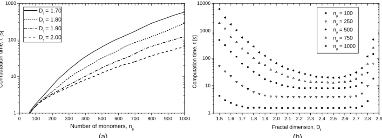
2.3.2.4.1 Computational time of DLA algorithm ... 431
2.4.1 A Comparison between DLA and DLCA aggregates ... 441
2.4.1.1 Numerical test sample of the DLCA aggregates ... 441
2.4.2.1 Estimation of the “global” fractal dimension ... 451
2.4.3.1 Non-homogeneity of the fractal dimension ... 471
2.4.4.1 Sticking DLA aggregates ... 481
2.5.1 Buckyballs aggregates ... 511
2.5.1.1 Introduction ... 511
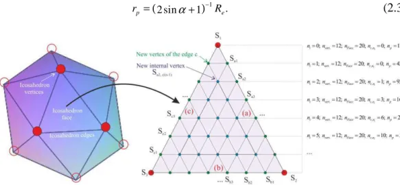
2.5.2.1 Geodesic dome model to describe Buckyballs morphology ... 521
2.5.2.1.1 Some important relations in the icosahedron ... 521
2.5.2.2.1 Building large and regular polyhedron ... 531
2.5.2.3.1 Projection of the circumscribed sphere ... 551
2.5.2.4.1 Optimization of the radius of each monomer ... 551
2.5.2.5.1 Filling Buckyballs ... 561
2.5.3.1 Numerical examples ... 561
2.6.1 Conclusion ... 581
3.1 TEM-BASED METHODS FOR THE ANALYSIS OF FRACTAL-LIKE
AGGREGATES ... 591
3.1.1 Introduction ... 591 3.2.1 Modeling and images pre-processing schemes ... 611
3.2.1.1 Modeling of TEM images ... 611
3.2.2.1 Overlapping factor and projection errors ... 641
TABLE OF CONTENTS
8
3.3.1 Methods for estimating the morphological parameters ... 671
3.3.1.1 Minimum Bounding Rectangle (MBR) method ... 671
3.3.1.1.1 Radius of gyration ... 681
3.3.1.2.1 Number of primary particles ... 701
3.3.1.3.1 Fractal dimension ... 711
3.3.2.1 Modified Box-Counting (MBC) method ... 711
3.4.1 Results and Discussion ... 741
3.4.1.1 The Minimum Bounding Rectangle (MBR) method ... 741
3.4.2.1 The Modified Box-Counting (MBC) method... 781
3.5.1 Conclusion ... 821
4.1 LIGHT SCATTERING THEORIES AND MODELS ... 831
4.1.1 Introduction ... 831 4.2.1 Lorenz-Mie theory ... 831
4.2.1.1 Solutions to the vector wave equations ... 841
4.2.2.1 The internal and scattered fields ... 851
4.2.3.1 Expressions for the phase functions and extinction cross sections ... 861
4.3.1 Rayleigh theory and Rayleigh-Gans-Debye (RGD) theory ... 871
4.3.1.1 Rayleigh theory ... 871
4.3.2.1 Rayleigh-Gans-Debye (RGD) theory ... 891
4.4.1 Rayleigh-Debye-Gans theory for Fractal Aggregates (RDG-FA) ... 911
4.4.1.1 General assumptions ... 911
4.4.2.1 Scattering intensity and cross sections ... 921
4.4.3.1 Scattering-extinction analysis ... 951
4.4.4.1 RDG-FA theory for soot aggregates ... 961
4.4.4.1.1 Numerical examples for the cross sections ... 971
4.4.4.2.1 Numerical examples for the scattering diagrams ... 1001
4.5.1 T-Matrix method... 1021
4.5.1.1 Introduction ... 1021
4.5.2.1 T-Matrix assumptions ... 1021
4.5.3.1 T-Matrix formulation ... 1031
4.5.4.1 The coordinate system and the displayed quantities ... 1051
4.5.5.1 Example numerical results ... 1051
4.5.5.1.1 Optical characteristics of various fractal aggregates ... 1051
4.5.5.2.1 Averaging procedure for the scattering diagrams ... 1071
4.5.5.3.1 Averaging procedure for the extinction profiles ... 1081
4.5.5.4.1 Extinction cross section of single monomers within fractal aggregates ... 1101
4.5.5.5.1 Extinction cross section of Buckyballs-like aggregates ... 1111
4.5.5.6.1 Extinction cross section of single monomers within Buckyballs aggregates ... 1121
4.5.5.7.1 Computational time with the T-Matrix code (Mackowski and Mishchenko 1996) ... 1131
4.6.1 Conclusion ... 1141
5.1 ANALYSIS OF THE SCATTERING DIAGRAMS ... 1151
5.1.1 Introduction ... 1151 5.2.1 Estimation of fractal parameters from scattering diagrams ... 1161
5.2.1.1 Introduction ... 1161
5.2.2.1 Light scattering properties ... 1161
9
5.2.4.1 Algorithms for estimating the fractal dimension ... 1171
5.2.4.1.1 Second Slope Estimation (SSE) Algorithm ... 1171
5.2.4.2.1 First Slope Estimation (FSE) Algorithm ... 1181
5.2.5.1 Results and discussion ... 1191
5.2.5.1.1 Estimation of the radius of gyration... 1201
5.2.5.2.1 Estimation of the fractal dimension ... 1211
5.2.6.1 Conclusion ... 1251
5.3.1 Influence of free monomers on the analysis of the OSF ... 1261
5.3.1.1 Physical background ... 1261
5.3.2.1 Results and discussion ... 1271
5.4.1 A comparison between scattering properties of DLA and DLCA aggregates ... 1291 5.5.1 Conclusion ... 1311
6.1 LIGHT EXTINCTION SPECTROMETRY (LES) ... 1331
6.1.1 Introduction ... 1331 6.2.1 Principle ... 1331 6.3.1 Inversion procedure ... 1351 6.4.1 Numerical results ... 1371
6.4.1.1 Extinction spectra and scattering diagrams ... 1371
6.4.1.1.1 Aggregates of Amorphous Silicon ... 1371
6.4.1.2.1 Aggregates of Silicon Dioxide ... 1401
6.4.1.3.1 Aggregates of Silicon Carbide ... 1431
6.4.2.1 Spectral transmission ... 1441
6.5.1 Experimental investigations ... 1461
6.5.1.1 Optical setup ... 1461
6.5.2.1 Aerosol of silicon dioxide buckyballs ... 1481
6.5.2.1.1 Setup: fluid loop and colloidal suspensions ... 1481
6.5.2.2.1 Inversion procedure ... 1511
6.5.2.3.1 Sampling procedure and electron microscopy analyses ... 1511
6.5.2.4.1 Experimental results ... 1511
6.5.3.1 Aerosol of tungsten aggregates ... 1591
6.5.3.1.1 Setup: fluid loop and powders ... 1591
6.5.3.2.1 Inversion procedure ... 1601
6.5.3.3.1 Example results ... 1601
6.5.4.1 Low-pressure discharge (dusty plasma) ... 1611
6.5.4.1.1 Background of the study ... 1611
6.5.4.2.1 Setup: plasma reactor and optical setup ... 1621
6.5.4.3.1 Experimental results ... 1631
6.6.1 Conclusion ... 1661
7.1 GENERAL CONCLUSION AND PERSPECTIVES ... 1671
8.1 REFERENCES ... 1701
RÉSUMÉ EN FRANCAIS (ABSTRACT IN FRENCH LANGUAGE) ... 1781
ABSTRAKT W J2ZYKU POLSKIM (ABSTRACT IN POLISH LANGUAGE) ... 1911
LIST OF SYMBOLS AND ABBREVIATIONS
10
LIST OF SYMBOLS AND ABBREVIATIONS
Symbols
TEM
δ the mean background noise and TEM image offset
0
λ laser wavelength in air
λ laser wavelength in the considered medium
θ scattering angle
x
σ standard deviation of x-value
p
σ standard deviation of particle radius
a subscript for aggregate
n
C particle concentration in number
v
C particle concentration in volume
x
C cross section (x = absorption, scattering or extinction)
2 3
,
D D
Cυκ Cυκ 2 and 3-dimensional overlapping factor of primary particles (monomers) in the
aggregate
2 3
, D D
dυκ dυκ 2 and 3-diemensional distance between centers of mass of primary particles
(monomers) p
d diameter of a single particle (monomer), dp =2rp
f
D fractal dimension of the aggregate
g gain of the optical conversion and imaging system
(
, g, f)
G k R D structure factor
i complex number
I scattering intensity
0
I incident beam intensity
( )
I q experimentally measured optical structure factor (OSF) of fractal-like
aggregate k wave number k=2 /π λ B k Boltzmann constant kB 1.381 10 23 [JK 1] − − ≈ × f
k fractal prefactor of the aggregate
p
k imaginary part of particle (monomer) refractive index at λ0 (kp ≥0)
m
K electron path length within external medium
p
K electron path length within particles (monomers)
L length of the experimental setup
2 D
11
3D
L total length of the aggregate in 3D space
e
m real refractive index of the external medium for λ0
p
m1 complex refractive index of particles (monomers) at λ0
p
m real part of the particle (monomer) refractive index at λ0
1, 2
M M the first and the second momentum (i.e. mean value and variance) of the
distribution of the number of monomers within aggregates p
n number of particles within an aggregate
p subscript for particles (monomers)
q magnitude of the scattering (wave) vector, q=2 sin( / 2)k θ
x
Q cross sections efficiency (x = absorption, scattering or extinction)
p
r radius of a single particle (monomer)
b
R minimum bounding sphere enclosing aggregate
e
R external boundary sphere used in the DLA algorithm
g
R radius of gyration of the aggregate
p
R appearance sphere used in the DLA algorithm
S
R radius in surface – radius of the sphere with surface equivalent to the one of the
aggregate (or particle)
v
R radius in volume – radius of the sphere with volume equivalent to the one of
the aggregate (or particle)
( )
S q structure factor of fractal-like aggregate
( )
iT λ beam transmission for λi wavelength
2D
W width of the 2D projection of the aggregate
3D
W total width of the aggregate in 3D space
p
x size parameter (i.e. Mie parameter), xp =2πrp/λ
Abbreviations and acronyms
abs subscript for absorption (cross section, efficiency, etc.)
ext subscript for extinction (cross section, efficiency, etc.)
sca subscript for scattering (cross section, efficiency, etc.)
DLA Diffusion Limited Aggregation
DLCA Diffusion Limited Cluster Aggregation
HC hexagonal close packed aggregate (hexagonal compact)
LIST OF SYMBOLS AND ABBREVIATIONS
12
LMT Lorenz-Mie Theory
Log.-Norm. Log-Normal size distribution
LSQ Least Square method
MBC Modified Box-Counting
MBR Minimum Bounding Rectangle
OSF Optical Structure Factor
PDF Probability Density Function
PSD Particle Size Distribution
RGD Rayleigh-Gans-Debye Theory
RDG-FA Rayleigh-Debye-Gans Theory for Fractal Aggregates
RLCA Reaction Limited Colloid Aggregation
SEM Scanning Electron Microscopy
TEM Transmission Electron Microscopy
13
1234567898
1.
INTRODUCTION
Undoubtedly, people have always been exposed to various nanoparticles via numerous natural phenomena, e.g. dust storms, volcanic ash, combustion, water evaporation, etc. At the same time, the human body has evolved to protect itself from potentially harmful influence of nanoparticles. However, from the technological point of view, for a long time we were not able to detect, control or use nanoparticles to any industrial application. The situation had
changed with rapidly developing technologies in the last decades of the 20th century.
Nowadays, nanoparticles and aggregates of nanoparticles are the subject of intensive research due to their unusual physical properties and potential technological impact. Basically, there are two primary factors that makes nanoparticles significantly different comparing to the bulk materials: surface effects and quantum effects (Buzea et al. 2007). Both of them influence any aspects related to the nanoparticles i.e. their chemical reactivity, mechanical, optical, electric and magnetic properties. In the same way, nanoparticles exhibit additional interesting and completely new properties, like strong ionic forces, unusual thermal diffusion or surface plasmons effects. They are also the subject of environmental and health concerns. Figure 1.1 shows some examples of nanoparticle aggregates encountered in various fields.
The surface effects are related to the fraction of atoms at the surface, which for nanomaterials is thousands of times larger than for the bulk ones. As an example, if we consider a single carbon microparticle with 60 mµ in diameter and 0.3 gµ mass, its surface area is equal to
2
0.01 mm (Buzea et al. 2007). To have the same mass in carbon nanoparticles with diameter
60 nm we need to take 1 billion particles. Their surface area is 2
11.3 mm giving the ratio surface area to the particles volume around 1000 times higher than for the single microparticle. As the particles reactivity is more and less determined by their surface, we can
CHAPTER 1 - INTRODUCTION
14
clearly see that reactivity of nanoparticles increases significantly comparing to the ordinary bulk materials, even at the microscale.
The quantum effects are related to the size of particles and appear as a sets of phenomena that are typical for single atoms rather than for particles or molecules (Roduner 2006). For instance, similarly as electrons in a single atom, quantum dots shows quantized energy spectra due to the electrons confinement. They demonstrate also quantified changes in their ability to accept or donate electrical charges. Yet another interesting result of the quantum confinement effect is that magnetic moments appear in nanoparticles of chemical compounds that are non-magnetic at a macroscale, e.g. gold, or platinum (Buzea et al. 2007).
Figure 1.1. Nanoparticles in various fields: (a) thermonuclear reactor and dust produced during the nuclear reaction, (b) plasma reactor and nanopowder, (c) nozzle to produce aerosols with spray drying method and highly-ordered Buckyballs aggregates, (d) flame and soot, (e) suspension and aggregation.
All the aforementioned issues cause that ultra-fine dry powders (nanometer-sized aggregates, ceramics and crystals, quantum dots), nano-colloidal suspensions (slurries, nanofluids, emulsions, gels) or nano-sized aerosols (various dusts, fine-droplet liquid paints, carbonaceous aggregates) are the milestones of the future science.
As already pointed out above, nanoparticles and aggregates of nanoparticles are highly interesting from the scientific and technological points of view. Nonetheless, to understand, to monitor and to control their properties and formation mechanisms in various systems, it is fundamental to access to key parameters like particle size distribution (PSD) and particle number concentration (Cn). But, this is precisely a challenge from the metrological and experimental points of view. Sampling and off-line analyses (e.g. electron microscopy, electro-mobility, etc.) are the most widely used methods to characterize properties of nano
15 and microparticles (i.e. size, shape, elementary composition and specific surface area). However, for so reactive and fragile objects, the reliability and repeatability of such analyses may be questionable. For instance, the sampling procedure can be biased by the particle flow-field dynamics or the smallest particles can remain trapped in micro roughness of the sampling tool or the substract (like in tokamaks). Apart from that, aggregates can be broken down due to the rolling and collapsing effects or by the sampling procedure itself. For all the above mentioned reasons, optical particle sizing techniques appear to be very suitable for the in-situ and the in-line characterization of the morphological properties of nanoparticle systems.
Various optical methods have been developed to characterize particle systems, e.g. (Xu 2002). However, using them to characterize complex particles is not an easy and trivial task. In the next paragraphs, to illustrate our purposes, the advantage and limits of four optical techniques used to characterize nanoparticles form in combustion and plasma systems are briefly reviewed.
- Particle Imaging Velocimetry (PIV) and Particle Tracking Velocimetry (PTV)
techniques (Stanislas et al. 2004) allow to measure the velocity of submicron particles. Both techniques relies on the illumination of the particle flow by two intense and successive pulsed laser sheets. The particles “image”, recorded by a CCD camera localized at θ = °90 , is just a bright spot whose size depends only on the point spread function (PSF) (Goodman 1996) of the imaging system. Using short time pulses (a few nanoseconds with a YAG laser) and a short time delays between the two successive pulses and images (down to few hundred nanoseconds with a typical PIV/PTV camera) allow to freeze particle motion and to measure velocities up to several hundred meters per second.
The only difference between PIV and PTV relies on the numerical algorithm used to obtain the velocity field. PIV estimates this field by measuring the global displacement of all particles within small interrogation windows (i.e. raw PIV images are meshed). Thus, based on a local flow field continuity assumption, PIV provides an Eulerian description of particulate media. On the other hand, PTV tracks each particle motion, providing an Lagrangian description of the particulate media (e.g. (Ouellette et al. 2006)). Therefore, PTV appears to be more appropriate for analyzing the spatial distribution of particles or particle properties linked to their charge and dynamics. Particle imaging techniques are basically constrained by the diffraction limit (Goodman 1996), making it impossible to image the surface and structure of sub-micron aggregates. Indeed, depth of view, optical magnification and aberrations, pixel size, particle size and refractive index, are also fundamental parameters that limit imaging technique capabilities.
However, imaging techniques can be used to characterize the size and the velocity of larger particles (see Figure 1.2 (a)). For this purpose, the PTV system must be operated in a backlight mode. In that configuration, the flow field is backlighted by a collimated beam,
CHAPTER 1 - INTRODUCTION
16
produced by a double pulse flash lamp or a laser. When a laser is used, a diffusion plate or a fluorescence cell must be used to decrease the speckle noise level (Guenadou et al. 2008). The CCD camera is equipped with high magnification optics and placed in front of the lighting
beam (i.e. θ= °0 ). With conventional systems, the minimum particle size that can be
“measured” is ≈4 mµ for a working distance of 4 mm≈ and a field of view of ≈400 400 m× µ 2
. These techniques have been extensively used to infer the size of nanoparticles in colloids or fusion plasmas (where the nanoparticles inter-distances or velocities are connected to their electrical charge, and then, their size) but they are not really of practical use for other systems (see Table 1.1) (Onofri et al. 2011b).
Figure 1.2. Basic experimental optical setups for (a) Shadowgraph imaging, Laser Light Scattering (LSS) and Ellipsometry techniques; (b) Light Extinction Spectroscopy (LES) and Laser Induced Incandescence (LII) techniques (Onofri et al. 2011b).
- Laser Induced Incandescence (LII) occurs when a laser beam encounters solid
absorbing particles (Melton 1984; Schulz et al. 2006; Michelsen et al. 2007; Vander-Wal 2009). The absorbed energy causes an increase of the particle temperature. Simultaneously, particles lose energy via heat transfer with their surrounding. If the energy absorption rate is sufficiently high, the temperature can reach high levels where significant incandescence (essentially blackbody emission) and vaporization phenomena can occur. The inversion of the LII signal intensity and time-decay is done with a PSD model assumption, allowing the determination of the volume concentration and the mean size of all single particles (referred also as monomers) and all small aggregates within the measurement volume. It can be a local (the detector is a photomultiplier, PM) or a 2D measurement (the detector is a streak camera, with a time resolution of a few nanoseconds (De-Iuliis et al. 2005; Desgroux et al. 2008)), see Figure 1.2 (b). The LII basic setup is then composed of a pulsed laser, a focusing optics, a collection (1D) or an imaging optics. Although, this technique is still under development, it has been used with success in combustion science (i.e. to characterize soots). It is however
Shadow. imag. Delay generator
LSS & Ellipsom. laser Shadow. imag. emission
Ellipsom. collection & polarization optics PM Shadow. imag. collection optics PM Polarization optics LSS:l/2; Nephel.:l/4 Rotative Linear polarizer 0-180° LSS-Goniometer, collection & polarization optics
Linear polarizer at 0° or 90° CCD camera Double pulse laser Fluorescence cell q 0° LII-Streak Camera LES - UV/NIR
Lamp & Spectrometer
LII-Delay generator LII-laser LII-1D Collection LES - Collection LII-Streak Camera LII-Streak Camera LII-2D Streak Camera Passband filter PM TTL Spatial filter LII-2D Collection LES - Emission L (a) (b) Fiber coupler Parabolic mirror On-line attenuator Optical fiber
17 fundamentally limited to extremely small absorbing particles at low concentration (see Table 1.1).
- The Laser Light Scattering (LLS) (referred also as the Nepholometry technique)
analyzes the angular scattering patterns produced by a sample of particles illuminated by focused and continuous laser beam, randomly or a linearly polarized (Xu 2002).
A LLS setup is generally, and basically, composed of a set of lenses, an interference filter centered onto the laser wavelength (to attenuate the optical background noise), a linear polarizer (to select parallel or/and perpendicular polarization), a spatial filter (to control the probe volume size) and a photomultiplier, see Figure 1.2 (a). Like most optical particle characterization techniques, LLS technique is limited to optically diluted particle systems although solutions have been proposed to correct multiple scattering effects with optical methods (Meyer et al. 1997; Onofri et al. 1999) or data inversion (Mokhtari et al. 2005; Tamanai et al. 2006). The main drawbacks of the LSS are that it cannot perform absolute particle concentration measurements, it requires wide optical accesses and a stationary process (i.e. regarding the scanning time). However, the LSS has two clear advantages: like the LII technique, it allows the detection of extremely small particles (e.g. monomers) at low concentration and, in addition, scattering diagrams are very sensitive to the morphology of aggregates (see Table 1.1 and reference (Onofri et al. 2011b) for additional inputs).
Table 1.1. Summary of key features of the various optical techniques.
Technique Shadow-imag. LES LII LSS Ellipsometry
Illumination system
Flash lamp, pulsed laser and
flurosc. cell, 0.1-100 mJ Stabilized thermal source, 5-20 W Pulsed laser, 50-700 mJ/cm2 continuous wave laser, 0.5-5 W continuous wave laser, 0.5-5 W Detection
system CCD camera Spectrometer PM or streak
camera Rotat. system, PM and polarizer PM with rotat. polarizer Size range 2 4 µm to cm 10 nm – 2 µm 2 nm – 0.5 µm 10 nm – 2 mm 10 nm – 2 µm
Concentration Relative Absolute Relative Relative Relative
Probe volume Slab, 10-2 mm3 –
102 cm3 Cylinder, cm3 – 104 cm3 Cubic or Slab, 10-3 mm3 – cm3 Cubic, 10-3 mm3 – cm3 Cubic, 10-3 mm3 – cm3 Main
advantage Flow pattern
size-velocity Limited access, long distance Low concentration Fractal dimension, low concentration Morphology, low concentration Main drawbacks
Only large par. depth of view, speckle noise Particle material spectrum needed Only monomers and dilute aggregates Wide optical access needed, Stationary flow Stationary flow, Local meas.
- Ellipsometry infers the properties of particles from their ability to modify the
CHAPTER 1 - INTRODUCTION
18
to produce a focused and polarized beam (i.e. circularly or linearly) that illuminates the particles within a small probe volume, see Figure 1.2 (a). Like the LSS, and for the same reasons, the collection optics is composed of a set of lenses, an interference filter, a spatial filter and a photomultiplier. Ellipsometry collection optics is ordinarily set at θ = °90 , and it integrates a computer controlled polarizing optics (e.g. a linear polarizer fixed on a motorized goniometer, or a liquid crystal linear polarizer). In most studies, the latter component is simply used to analyze the light polarization phase-angle 1 and amplitude 3 (e.g. (Hong and Winter 2006)). Based on the Lorenz-Mie calculations, the inversion procedure consists on searching for the particle mean diameter and refractive index that allow to minimize differences observed between the theoretical and experimental values of 1 and 3 (Mishchenko et al. 2000). Indeed, light polarization is very sensitive to particle roughness and heterogeneity, making polarization techniques suitable for particle morphology investigations provided that an appropriate scattering models (like the T-Matrix or the DDA ones) is used. Among the drawbacks of this technique there is the fact that the measurement is local and that it requires well defined optical accesses, see Table 1.1 (Onofri et al. 2011b). The latter constraint make this technique totally unsuitable to characterize, for instance, dust in fusion devices.
One can conclude that very few methods allow the in-situ and time-resolved analysis, with limited optical accesses, of nanoparticle systems, and if there are, they usually use too simple light scattering model and inversion technique.
So that, the goal of this Ph.D. work was to contribute to the development of the two aforementioned optical methods: the Light Extinction Spectrometry (LES) and the Laser Light Scattering (LLS), and this, by using realistic and as accurate as possible particle and light scattering models, by developing dedicated inversion methods and validation experiments. All this work has been done with the objective to propose in fine an optical diagnosis that can be used both to perform laboratory experiments (mainly on colloidal suspensions) and experiments at long distance (fusion devices, aerosols, combustion).
Chapter 2 introduces the particle models we have developed to describes the morphology of two types of nanoparticle aggregates of interest, and with a fractal-like (plasmas, combustion systems) and buckyballs-like (aerosols, suspensions) shapes.
Chapter 3 summarize all the work done to determine the morphological parameters of fractal-like aggregates from electron microscopy images.
Chapter 4 reviews and discuss the physical and mathematical backgrounds of all the theories used in this work to predict the light scattering properties of nanoparticle and their aggregates: Lorenz-Mie theory, Rayleigh-based approximations (RGD, RDG-FA) and T-Matrix method.
19 Chapter 5 presents the algorithms and results obtained for the extraction of the morphological parameters of fractal aggregates from their scattering diagrams, the influence of single particles or the superposition of different populations of aggregates.
Chapter 6 details the basic principles as well as inversion techniques of extinction data recorded for fractal-like and buckyballs-like aggregates. Various experimental systems are considered and analyzed: aerosol of silica nanobeads and tungsten aggregates, dusty plasmas with silicone aggregates.
Chapter 7 is a general conclusion with perspectives for this work. Chapter 8 contains references.
Chapter 9 and 10 are extended abstracts of this work, in French and in Polish languages respectively.
20
12345678A8
2.
MODELS FOR PARTICLE AGGREGATES
2.1.
Introduction
Aggregation of nanoparticles occurs in numerous media and it has significant influence on the overall properties of the particle systems. For instance, although the chemical reactions and physical processes governing combustion systems, dusty plasmas or colloidal suspensions may be considered as rather different, they can lead to the formation of aggregates of nanoparticles with similar shapes. Nevertheless, from one case to another, the clusters may exhibit highly different dimensions or morphological properties. For example, they may contain from a few primary particles (called also monomers) up to several thousands of them. They may also take various shapes: from the dilute chain-like formations (Kim et al. 2003), through the typical fractal-like aggregates (Sorensen 2001), up to the dense and opaque cauliflower-like structures (Sharpe et al. 2003; Onofri et al. 2011b). To describe very dense and highly opaque aggregates with an overall shape close to the spherical one, buckyballs model (see section 2.5) (Toure 2010) may be applied. For highly ordered crystal structures one can also use hexagonal compact particle model (Holland et al. 1998).
The chapter is organized as follows. Section 2.2 presents a simplified overview of the physical background of the aggregation phenomena for colloidal suspensions according to the DLVO model. Section 2.3 is devoted to the numerical algorithm of the Diffusion Limited Aggregation (DLA) we have developed to reproduce the morphology of fractal-like aggregates. Section 2.4 compares DLA aggregates produced with our tunable algorithm with numerically generated DLCA aggregates provided by Dr. Jérôme Yon. Section 2.5 describes a mathematical and physical model to reproduce the morphology of highly ordered aggregates.
21
2.2.
Physical basis of the aggregation in colloidal suspensions
2.2.1.
Aggregation regimes
To characterize particle motion in a medium, the most commonly used parameter is the
Knudsen number. It combines the mean free path l and the radius rp of the particle:
. p l Kn r = (2.1)
We define also the diffusion Knudsen number as KnD =lp/rp, where lp is the persistence length of the particle (i.e. the distance over which a particle moves effectively in a straight line). Depending on the values of the Knudsen number, three different aggregation regimes are defined (Pierce et al. 2006): the “continuum regime” (referred also as the “Stokes” or
“hydrodynamic regime”, Kn 2 ), the intermediate regime (called also the “slip regime”,1
~ 0
Kn ) and the “free molecular regime” (Kn 3 ). 1
Most aggregation studies have been carried out in the continuum regime (Kn 2 ), where 1 particles motion between collisions is diffusive. This regime refers to aggregation in colloidal liquid suspensions or aerosols at low temperature and high pressure. In the continuum regime each particle experience a drag force that, for spherical particles, can be calculated as:
6 p,
f = πηr (2.2)
where η is the dynamic viscosity of the medium. The diffusion constant for spherical
particles is described by the Stokes-Einstein equation (Pierce et al. 2006):
, 6 B SE p k T D r πη = (2.3)
where kB is Boltzmann’s constant and T is the medium temperature.
In the free molecular regime (Kn 3 ) monomers have a similar mean free path as the 1
molecules of the surrounding medium and the distance between monomers is significantly large. Due to the law describing the drag force of particles, this region is also called the Epstein regime. In this regime, the drag force of a single monomer is:
1/ 2 2 2 8 1 , 3 8 m B p m k T f r m β π π ρ1 2 1 2 = 3 4 3 + 4 5 6 5 6 (2.4)
where ρ is the medium mass density, mm is the molecular mass of the particles and βm is the
momentum accommodation coefficient. In the free molecular regime monomers move either ballistically or diffusively (Meakin 1984; Stasio et al. 2002; Babu et al. 2008). Usually, the limit between the diffusive and the ballistic motion, is found for diffusion Knudsen number smaller than KnD ≈1. In that case, the diffusion constant is given by (Pierce et al. 2006):
CHAPTER 2 - MODELS FOR PARTICLE AGGREGATES 22 1/2 1 2 3 1 . 8 2 8 m B Ep m p m k T D r π β ρ π − 1 2 1 2 = 3 4 3 + 4 5 6 5 6 (2.5)
During the ballistic motion the root mean square velocity of the monomers with mass m can
be calculated as (Pierce et al. 2006):
1/ 2 3 . B k T v m 1 2 =3 4 5 6 (2.6)
The intermediate regime (slip regime) is observed for 0.1≤Kn≤10 (Pierce et al. 2006). Particles motion in this regime may be described introducing the Cunningham correction
( )
C Kn into the Stokes-Einstein equations. Therefore, the diffusion constant is given as:
( )
,SE
D=D C Kn (2.7)
with the corresponding drag force:
( )
6 . p r f C Kn πη = (2.8)Eqs. (2.1) – (2.8) refer to a single particle in various aggregation regimes. Nevertheless, they can be also apply to fractal aggregates. To do so, one must take into account that fractal aggregates are ramified, so to estimate the drag force or the diffusion constant, we must
introduce the effective mobility radius Rm. In that case, regardless of the aggregate
morphology, we can use Eqs. (2.1) – (2.8) with the Rm instead of the rp.
2.2.2.
Aggregation models (DLA, DLCA, RLCA)
In colloidal suspensions particles remain in a constant motion caused by the molecular collisions. This phenomenon, studied independently by Albert Einstein (1905) (Einstein 1956) and Marian Smoluchowski (1906) (Smoluchowski 1906), is widely known as the Brownian motion. Each particle experience a random walk like the one simulated on Figure 2.1. The latter figure shows 5000 steps of the motion of a single monomer in 3-dimensional space. Length scale in the presented figure is normalized by the step increment of the particle (i.e. increment step is equal to 1).
23 -40 -30 -20 -10 0 10 -50 -40 -30 -20 -10 0 10 20 -40 -30 -20 -10 0 10 Z Y X
Figure 2.1. Simulated Brownian motion: 5000 steps of a single monomer in a 3-dimensional space (increment step equal to 1).
According to the DLVO model, the suspension remains stable against the aggregation (Lin et al. 1989), if the repulsive energy barrier caused by the electrostatic forces is much greater than
B
k T (where kB is the Boltzmann constant and T is the temperature). In that case attractive,
short-range van der Waals forces (proportional to the 6
1 / r , where r is a distance from the particle) are much weaker than the repulsive long-range, electrostatic forces between
monomers (proportional to the 2
1 / r ). To make the suspension unstable and hence trigger aggregation phenomena, we can modify the ionic balance of the system by changing the pH (neutralize the surface charges of the particles) adding tensio-actives to reduce the range of the electrostatic forces, etc. When the attractive van der Waals forces are no more balanced – they predominate causing aggregation. For dilute particle system the dynamics of this aggregation process is fundamentally limited by the ability of the primary particles to diffuse within the continuous medium, so that it is usually referenced as the Diffusion Limited Aggregation (DLA, e.g. (Witten and Sander 1981; Jullien and Botet 1987)). In that case, due to large distances between particles, diffusion of aggregates within a continuous medium is negligible. It is important to notice that in the suspension where repulsive energy barrier is greater than several k TB particles are still able to stick together but significant number of
collisions is necessary. This is the fundamental requirement for the Reaction-Limited Colloid Aggregation (RLCA) (Lin et al. 1989). In contradiction to that, for the DLA process probability that two colliding particles stick together is close to unity. During the aggregation not only single monomers but also previously formed aggregates may collide. The process in which the DLA phenomena and clusterization occur simultaneously is called the Diffusion-Limited Cluster Aggregation (DLCA, e.g. (Weitz et al. 1985; Tang et al. 2000; Babu et al. 2008)). Its dynamics is limited by the ability of the previously formed clusters to diffuse within the continuous medium.
CHAPTER 2 - MODELS FOR PARTICLE AGGREGATES
24
In the current part of this work, to generate synthetic aggregates, an fully adjustable (tunable) DLA-type code has been developed rather than a DLCA one. The main reason for that is that presented research requires aggregates with precisely defined parameters, strict self-similarity and thus scale-invariant properties (Theiler 1990). This requirement is not precisely satisfied for small aggregates produced in DLCA model (i.e. the power law nature of Eq. (2.13) is not satisfied) (Heinson et al. 2010). Furthermore, DLCA models should take into account physical (e.g. van der Waals’, Coulomb's forces), mechanical (e.g. excluded volume, entanglement) and chemical (e.g. sintering, bonding) interactions and mechanisms that are not yet fully understood. But this is not the case as most DLCA as well as DLA models described in the literature assume only random motion of monomers and an irreversible sticking after their collision. They do not require any initial constraints regarding fractal dimension, fractal prefactor or number of monomers within aggregates. When simulation process is completed, the fractal parameters of the generated aggregates may be calculated.
The biggest advantage of the tunable DLA code developed in the current work is that it preserves all the fractal parameters (with a given accuracy) at each step of the aggregation process. This allows to avoid generation of multi-fractal aggregates (i.e. aggregates with different parameters at different scale or in a different part of the particle) and assures reliability and repeatability of the results. The detailed description of the DLA software and algorithm applied in this work can be found in section 2.3.
2.2.3.
Scaling law for the aggregate growth rate
A complete characterization of the aggregating system requires to define aggregation kinetics and the structure of the growing aggregate. The cluster-cluster aggregation kinetics is governed by Smoluchowski equation (Zift et al. 1985). For sufficiently dilute systems of monodisperse monomers the Smoluchowski equation may be expressed in the relatively simple form (Sorensen et al. 1998; Stasio et al. 2002):
2 1 , 2 n c n dC K C dt = − (2.9)
where Kc is the aggregation kernel, which specifies the aggregation rates, and Cn is the
particle number concentration. The aggregate structure is well described by the number of monomers np, their mean radius rp and the related PSD, as well as the fractal parameters: Df,
f
k and Rg (see Eq. (2.13) and description later on).
The aggregation kinetics may be characterized by the time evolution of the average mass of
the aggregate z
m4t . For the DLCA in colloidal suspension, the linear dependency of the
aggregation kinetics was observed (Lin et al. 1989), so that z=1 and
(
/ 0)
z
m= t t . Characteristic time t0 is given by t0 =3 / 8η
(
k TCB n,0)
, where η is the dynamic viscosity of thefluid and Cn,0 is the initial particle concentration. The aggregate mass distribution during the
25 and Benedek 1982) which, with a good approximation, leads to the solution expressed by the following exponential form:
1 1 ( ) 1 , m a n n m m m − 1 2 = 3 − 4 5 6 (2.10)
where na =
7
n m( ) is the total number of aggregates and m=7
mn m( )/na is the mean mass ofthe aggregates.
Although there are initial similarities between the diffusion-limited and the reaction-limited cluster aggregation phenomena, both processes appear to be considerably different. The time
evolution of the average mass of the aggregate in the RLCA is defined as m eAt
4 , where A is
a constant dependent on the sticking probability and the time between collisions of monomers. On the other way, the solution of Smoluchowski equations is given as:
/ ( ) m mc,
n m 4m e−τ − (2.11)
where τ is a constant evaluated analytically, numerically and experimentally in the range 1.5 1.9
τ = − (Lin et al. 1989).
2.3.
DLA aggregates
We define here aggregates as objects made of small elementary particles (monomers) that are stuck together and form a larger structure. It was shown that to describe and analyze aggregated particles we can apply the fractal-like model (Witten and Sander 1981). Its main concept is based on the self-similarity and structure invariance at each scale. The fractal theory may be applied regardless of the particular aggregation phenomena and specific conditions that have led to the cluster formation (Weitz and Oliveria 1984). Following this approach, in the fractal-like model the mass of the cluster M and its spatial dimension L, may be simply related as:
,
D
M4L (2.12)
where D is the Hausdorff or the so-called fractal dimension. It is always smaller than the Euclidian dimension. This relation describes the basic concept of the fractal-like aggregates and it is the fundamental dependency applied in the further morphological analysis.
2.3.1.
Numerical model and algorithm of DLA aggregates
To define mathematically, and by a limited number of parameters, the morphology of particle aggregates, the so-called fractal equation (Forrest and Witten 1979; Bau et al. 2010) is commonly used: , f D g p f p R n k r 1 2 = 33 44 5 6 (2.13)
CHAPTER 2 - MODELS FOR PARTICLE AGGREGATES
26
where np and rp represent respectively the number and the mean radius of the primary
particles (monomers), Df and Rg are the fractal dimension and the radius of gyration of the
aggregate, and kf is called the fractal prefactor (or structural coefficient).
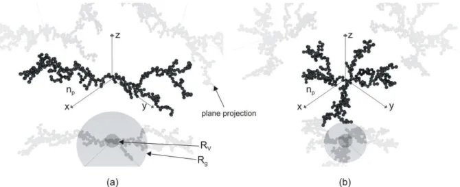
Figure 2.2. Numerically generated fractal aggregate with parameters: np=100,Df =1.80,kf =1.593,
9.97
g
R = , Rv = 4.64: (a) 3D rendering with POV-Ray software, (b) 2D projection of the aggregate.
As an example, Figure 2.2 (a) shows a 3D visualization (created with the POV-Ray software
(POV-Ray 2004)) of the aggregate defined by np =100 monomers, fractal dimension
1.80
f
D = , fractal prefactor kf =1.593, radius of gyration Rg =9.97 and equivalent radius in volume Rv =4.46. Figure 2.2 (b) shows a 2D projection (the image of the aggregate as it is obtained in the zy plane).
In Eq. (2.13), and more particularly in this work, the fractal dimension and the radius of gyration are thought to be the key parameters to describe the morphology of aggregates. To define the radius of gyration, the centre of mass of the aggregate
(
x y za, a, a)
must be previously specified. For the group of particles it may be defined as follows:(
)
1 1 1 1 1 , , , , , p p p p n n n a a a n n n n n n n n n n n n x y z x m y m z m m = = = = 1 2 = 33 44 57
7
7
67
(2.14)where
(
x y zn, n, n)
is the vector pointing to the n th− particle with mass mn. If we assume thatall particles have the same unitary mass and radius m0 and r0 respectively, we can define the
mass of the n th− particle with radius rp n, as 3
0 ,
n p n
m =m r . Using this assumption we can
eliminate the mass of the particles in Eq. (2.14). The position of the centre of mass is now defined, so we can calculate the aggregate’s radius of gyration. The latter quantity characterize the spatial distribution of mass in the aggregate. It is defined as a mean square distance of the particles from the centre of mass:
2 1 1 ( ) , p n g n p R n = =
7
r0−rn (2.15)27 where in the classical laboratory Cartesian and Spherical Coordinate Systems
(
x y z, ,)
and(
r, ,θ ϕ)
, rn and r0 are vectors pointing respectively the n th− particle and the centre of massof the aggregate with radius of gyration Rg.
2.3.1.1. Aggregation algorithm
Figure 2.3 shows a flow chart of the DLA algorithm. An overview diagram of the geometry of the DLA algorithm is shown in Figure 2.4 (a). In the aggregation process all the primary particles are generated successively at a large distance Rp (also called appearance sphere) from the centre of mass of the aggregating
cluster: , p, p g n R 3 R (2.16) where , p g n
R describes the temporary radius of
gyration of the growing aggregate. If during its random march the new particle moves out of the external boundary sphere with radius Re,
the particle is rejected and another particle is generated at the distance Rp. The definition of
the boundary sphere with radius Re, with
e
R ≥Rp (ideally Re3Rp) is necessary to avoid particle’s roaming far from the aggregate since this will significantly increase computational time. It is important to notice that here, the radiuses of appearance and external boundary spheres are not fixed. These values are continuously optimized. To do so, they are calculated as the sum of the additional
constants (p and b for the appearance and the
boundary spheres respectively) and multiplied by the radius of the minimum bounding sphere and by a factor called “appearance sphere multiplier”. This procedure provides a wide range of possible relations between the Rb, Rp and Re. For example, it is possible to turn off
the multiplication and use only a constant difference between radiuses of the defined spheres.
Figure 2.3. Schematic diagram of the DLA algorithm.
CHAPTER 2 - MODELS FOR PARTICLE AGGREGATES
28
Figure 2.4. (a) Schematic diagram of the Diffusion Limited Aggregation (DLA) steps and parameters and (b) Spherical Coordinate System.
Figure 2.4 (b) presents the coordinate system of the DLA code. To avoid problems related with temporary position of the growing cluster at each step of the algorithm the centre of mass of the aggregate is relocated at the centre of the coordinate system. When the aggregation procedure is completed it is necessary to convert the spherical coordinates
(
r, ,θ ϕ)
to theclassical laboratory Cartesian Coordinate System
(
x y z, ,)
. To do so we can use the followingmapping procedure: cos sin , sin sin , cos . x r y r z r θ ϕ θ ϕ ϕ = = = (2.17)
The random motion of the primary particles is simulated by the decomposition of their trajectories into small step increments (e.g. 2rp) with a statistically true isotropic orientation.
The latter is obtained by generating at each step random inclination and azimuth angles ϕ θ,
with a uniform spherical distribution (Bird 1994). This procedure is not a trivial task because the intuitive approach is incorrect. Indeed, if we generate the inclination and azimuth angles
,
ϕ θ in the range
[ ]
0,π and[
0, 2π]
respectively and transform them to the Spherical Coordinate System using Eq. (2.17), the points are not distributed uniformly. As an example, Figure 2.5 shows 5000 points generated on the surface of a unit sphere. It can be seen that their spatial distribution is denser at the poles. This problem is caused by the mapping procedure between the spherical and the Cartesian coordinates which does not preserve area (i.e. initial space is pinched and compressed at the poles). It is clear that random numbers generated in this way would strongly affect aggregation procedure and thus generated aggregates would be statistically elongated and oriented (anisotropic).x y z φ θ P O r Accepted monomer Minimum bounding sphere, Rb
Random walk
New monomer
Aggregate
Appearance sphere, Rp
External boundary sphere, Re
Rejected monomer
(b) (a)
29 -1.0 -0.5 0.0 0.5 1.0 -1.0 -0.5 0.0 0.5 1.0 -1.0 -0.5 0.0 0.5 1.0 (a) Z A x is Y Ax is X Axis -1.0 -0.5 0.0 0.5 1.0 -1.0 -0.5 0.0 0.5 1.0 (b) Y a x is X axis 0 1 2 3 4 5 6 0.0 0.5 1.0 1.5 2.0 2.5 3.0 (c) V e rt ic a l a n g le , ϕ Horizontal angle, ϑ
Figure 2.5. 5000 points generated on a surface of a unit sphere with the Uniform Distribution in the Cartesian Coordinates mapped to the Spherical Coordinate System: (a) 3D view, (b) top view of the region of the “north” pole and (c) angular distribution of the points.
-1.0 -0.5 0.0 0.5 1.0 -1.0 -0.5 0.0 0.5 1.0 -1.0 -0.5 0.0 0.5 1.0 Z A x is Y Ax is X Axis (a) -1.0 -0.5 0.0 0.5 1.0 -1.0 -0.5 0.0 0.5 1.0 Y a x is X axis (b) 0 1 2 3 4 5 6 0.0 0.5 1.0 1.5 2.0 2.5 3.0 (c) V e rt ic a l a n g le , ϕ Horizontal angle, ϑ
Figure 2.6. 5000 points generated on a surface of a unit sphere with the Uniform Spherical Distribution: (a) 3D view, (b) top view of the region of the “north” pole and (c) angular distribution of the points.
To avoid orientation problem and to find equations necessary for the generation of random points with the Uniform Spherical Distribution, it is necessary to consider the Jacobian matrix of the mapping procedure (Bird 1994):
(
, ,)
cos sinsin sin cos cossin cos cos sinsin sin .cos sin cos
F x x x r r r y y y J r r r r r z z z r ϕ θ θ ϕ θ ϕ θ ϕ ϕ θ θ ϕ θ ϕ θ ϕ ϕ θ ϕ ϕ ϕ ϕ θ 8∂ ∂ ∂ 9 A∂ ∂ ∂ B A B 8 − 9 A∂ ∂ ∂ B A B =A B A= B ∂ ∂ ∂ A B AC − BD A∂ ∂ ∂ B A B ∂ ∂ ∂ C D (2.18)
The Jacobian determinant is independent of the azimuth angle θ but it is related with the inclination angle ϕ and radius r. However, if we consider an unit sphere we can cut out
CHAPTER 2 - MODELS FOR PARTICLE AGGREGATES
30
cumulative distribution function. Finally, using its inverse we can generate the inclination and
azimuth angles ϕ θ, with uniform spherical distribution (Bird 1994):
1 2 2 , 2arcsin , θ πδ ϕ δ = = (2.19)
where, δ1 and δ2 are uniform distributions on
[ ]
0,1 . As an example, Figure 2.6 shows 5000points generated on a surface of a unit sphere. It is worth to compare the distribution of the
angles ϕ and θ generated with both solutions (see Figure 2.5 (c) and Figure 2.6 (c)). It can be
seen that now, the points are distributed equally on the entire surface of the given sphere (Figure 2.6).
2.3.1.2. Sticking process
Figure 2.7 shows a schematic diagram of a collision between a randomly marching monomer and an aggregating cluster. It should be noticed that for drawing considerations the increment step presented here (equal to 6rp) is significantly larger than the one used for our simulations (see Table 2.1). If the distance between the current position of the monomer (a) and any of the particles within the aggregating cluster is smaller than the increment step, the possibility of a collision must be considered. In that case, new coordinates of the monomer (b) are calculated with the typical procedure described above. However, the algorithm also verifies whether during the current increment step (i.e. between positions (a) and (b)) the monomer collides with the aggregate or not. If an intersection occurs (see Figure 2.7), the coordinates of the marching particle are recalculated the exact contact position (c).
Figure 2.7. Schematic diagram of a collision between a randomly marching monomer and aggregating cluster: (a) current position of the monomer, (b) new position of the monomer without collision, (c) position of the monomer at the collision point.
The procedure described above does not fulfill all requirements for the aggregation process. In fact, the collision and sticking between a single monomer and an aggregate of np−1
particles, is only effective when the following inequality is satisfied:
, , , 1 , 1 , 1 f f p p p p D D g n p g n g n p g n R n R R n R ε ε − + − − 1 2 1 2 3 4 ≤ ≤3 4 3 4 − 3 4 5 6 5 6 (2.20) (a) (c) (b) Marching monomer Aggregating cluster Increment step
31 where 4 is an accuracy parameter on the fractal dimension. In the DLA software this value
may be adjusted on demand. Nevertheless, in the present study it was fixed at 2
10
ε = −
as smaller values greatly increase computational time without noticeable improvements in morphological characteristics of the aggregates. Something important to understand is that Eq. (2.20) allows ensuring at each aggregation step that Eq. (2.13) is nearly verified and thus, that the scaling properties of all aggregates are conserved at all scales.
During the aggregation process we assume that particles stick together like hard spheres in contact, i.e. exactly in one point and any additional displacement after their collision is impossible. From a macroscopic point of view both assumptions, especially the latter, seem to be incorrect. It is obvious that velocity of a fast moving object after a collision with a larger one decreases significantly but due to the principle of inertia and the law of conservation of the linear momentum, the colliding particle should in most cases remains in motion. This is not necessarily the case of nanoparticles which are mostly sensitive to adhesion and short range forces (e.g. Van der Waals forces). Nevertheless, it is common to simplify this problem and ignore particle displacement after collision (Witten and Sander 1981; Babu et al. 2008).
2.3.1.3. Overlapping factor
In some particle systems, due to additional processes (e.g. melting, polymerization, deposition or collision impact), primary particles may be entangled by more than a single point of contact, and they can also significantly overlap. For example, overlapping may be encountered when aggregation process occurs at high temperature (e.g. during combustion or in a plasma system), so it may be necessary to take into account and model this phenomenon. Figure 2.8 shows a schematic diagram of the overlapping of 2 particles with radiuses rp,1, rp,2
and their centers of mass distant each other by d3D
12.
Figure 2.8. Schematic diagram of the three dimensional overlapping factor Cυκ3D for 2 spherical particles with radiuses rp1, rp2 and their centers of mass distant each other by d123D.
To quantify overlapping effect, it is convenient to define a 3D overlapping factor based on the true Euclidian inter-distance d3D
12 between the particles' centers of mass (Brasil et al. 1999):
(
)
3 ,1 ,2 3 ,1 ,2 , D p p D p p r r d C r r υκ υκ + − = + (2.21)CHAPTER 2 - MODELS FOR PARTICLE AGGREGATES
32
where Cυκ3D <0 for monomers that are not in contact, Cυκ3D =0 for hard spheres in contact and
(
]
30,1
D
Cυκ ∈ for partially to fully overlapped spheres. If we consider only monodisperse
particles within an aggregate, Eq. (2.21) may be simplified to:
(
)
3 3 2 / 2 . D D p p Cυκ = r −dυκ r (2.22)As an example, for diesel soot aggregates, depending on the sampling and storage protocols, Wentzel et al. (Wentzel et al. 2003) have found an overlapping factor in the range
3
0.10 0.29 D
Cυκ = − , while Ouf et al. (Ouf et al. 2010) reported Cυκ3D =0.16 0.30− . We have found
similar value (Cυκ3D =0.20 0.05± ) for the experimental sample of diesel soot particles (Yon et al. 2011) during the TEM-based analysis (see chapter 3). Estimated overlapping factor was also applied to model artificial fractal-like aggregates.
In what follows, to numerically account for overlapping (Brasil et al. 1999), we first generate an aggregate of hard spheres in contact. Next, we can take into account for Cυκ3D by progressively increasing the radiuses of monomers within an aggregate while maintaining the position of their centers. At the same time it is necessary to perform a scaling down procedure to keep the initial value of the particle radius. Described steps are depicted in Figure 2.9.
Figure 2.9. Numerical procedure for overlapping: (a) an aggregate with hard spheres in contact, (b) the aggregate with expanded radiuses of monomers, (c) the aggregate after scaling down procedure.
Figure 2.10 compares radius of gyration of the aggregates with fractal dimension equal to 1.80 and various number of monomers for different overlapping factors (from 0 to 0.5). It can be seen that the overlapping factor has a linear influence on the radius of gyration.