HAL Id: tel-02408685
https://hal.archives-ouvertes.fr/tel-02408685
Submitted on 13 Dec 2019HAL is a multi-disciplinary open access archive for the deposit and dissemination of sci-entific research documents, whether they are pub-lished or not. The documents may come from teaching and research institutions in France or abroad, or from public or private research centers.
L’archive ouverte pluridisciplinaire HAL, est destinée au dépôt et à la diffusion de documents scientifiques de niveau recherche, publiés ou non, émanant des établissements d’enseignement et de recherche français ou étrangers, des laboratoires publics ou privés.
System: the case of Guanay cormorant, Peruvian booby
and Peruvian pelican
Giannina Paola Passuni Saldana
To cite this version:
Giannina Paola Passuni Saldana. A bird-eye view on the spatio-temporal variability of the seasonal cycle in the Northern Humboldt Current System: the case of Guanay cormorant, Peruvian booby and Peruvian pelican. Biodiversity and Ecology. Université de Montpellier, 2016. English. �tel-02408685�
Délivré par l’Université de Montpellier Préparée au sein de l’école doctorale
GAIA : Biodiversité, Agriculture, Alimentation, Environnement, Terre, Eau
Et de l’unité de recherche Marine Biodiversity, Exploitation and Conservation
Spécialité : Ecosystèmes et sciences agronomiques Présentée par Giannina Paola Passuni Saldana
Soutenue le 15 avril devant le jury composé de
M. Ronan FABLET, Professeur, Universite de Bretagne Occidentale
Rapporteur
M.Daniel ORO, Directeur de Recherche, Consejo Superior de Investigaciones Cientificas
Rapporteur
M. Etienne DANCHIN, Directeur de Recherche, CNRS
Examinateur
M. Alexis CHAIGNEAU, Chargee de Recherche, IRD
Examinateur
M. Thierry BOULINIER, Directeur de Recherche, CNRS
Examinateur
M.Christophe BARBRAUD, Charge de Recherche, CNRS
Co-directeur de these
Mme.Sophie BERTRAND, Charge de Recherche, IRD
Directrice de these
A bird-eye view on the spatio-temporal
variability of the seasonal cycle in the
Northern Humboldt Current System: the case
of Guanay cormorant, Peruvian booby and
Peruvian pelican
celeste magnitud, innumerable emigración del viento de la vida, cuando vuestros cometas se deslizan enarenando el cielo sigiloso
del callado Perú, vuela el eclipse. Oh lento amor, salvaje primavera que desarraiga su colmada copa y navega la nave de la especie
con un fluvial temblor de agua sagrada desplazando su cielo caudaloso
hacia las islas rojas del estiércol. Yo quiero sumergirme en vuestras alas, ir hacia el Sur durmiendo, sostenido por toda la espesura temblorosa. Ir en el río oscuro de las flechas con una voz perdida, dividirme en la palpitación inseparable.
Después, lluvia del vuelo, las calcáreas islas abren su frío paraíso
donde cae la luna del plumaje, la tormenta enlutada de las plumas. El hombre inclina entonces la cabeza ante el arrullo de las aves madres, y escarba estiércol con las manos ciegas que levantan las gradas una a una, raspa la claridad del excremento, acumula las heces derramadas, y se prosterna en medio de las islas de la fermentación, como un esclavo, saludando las ácidas riberas
que coronan los pájaros ilustres.
The Northern Humboldt Current System (NHCS) is a place of a high biological activity due to an intense coastal upwelling. It supports one of the biggest forage fish populations, the Peruvian anchovy, and the world-leading monospecific fishery in terms of landings. The NHCS also hosts large, although variable, seabird populations, composed among others by three guano-producing sympatric species: the Guanay cormorant (Phalacrocorax bougainvillii), the Peruvian booby (Sula variegata) and the Peruvian pelican (Pelecanus thagus), which all feed primarily on anchovy.
In this work we reviewed the fluctuations of these three seabird populations, focusing on the seasonal cycle of their breeding, to address the following questions: How different are the seasonality of reproduction among species? To what extent may they be plastic in space and time? What from the natural environment and the anthropogenic activities impact more the breeding of seabirds?
We addressed these questions using the monthly occupancy of breeders (1) in >30 Peruvian sites between 06°S and 18°S and from 2003 to 2014; and (2) in one site during three decadal periods (1952-1968, 1972-1989, 2003-2014). We also used environmental covariates from satellite and at-sea monitoring such as oceanographic conditions, prey abundance, availability and body conditions, and fisheries pressure covariates. We used multiseason occupancy models to characterize the seasonality of breeding and relate it with environmental covariates. We also used functional principal component analysis for classifying the differences in seasonality among sites, and random forest regression for analyzing the relative contribution of covariates in the variability of the seasonal breeding.
We found that in average seasonal breeding mainly started during the austral winter/ early spring and ended in summer/ early fall, this pattern being stronger in boobies and pelicans than in cormorants. The breeding onset of seabirds is timed so that fledging independence occurs when primary production, prey conditions and availability are maximized. This pattern is unique compared with other upwelling ecosystems and could be explained by the year-round high abundances of anchovy in the NHCS.
The average seasonal breeding may differ among nesting sites. Seabirds breed earlier and are more persistent when colonies are larger, located on islands, within the first 20km of the coast, at lower latitudes and with greater primary production conditions. These results suggest that in the NHCS, the seasonality of breeding is more influenced by local environmental conditions than by large-scale environmental gradients. These results provide critical information to a better coordination of guano extraction and conservancy policies.
Seabirds may also adapt the seasonality of their breeding to drastic ecosystem changes caused by regime shifts. We found that the three study species exhibited a gradient of plasticity regarding the seasonality of their breeding. Cormorants showed a greater plasticity, modulating the timing
may be related to their specific foraging strategy and/or to changes of prey items when anchovy stock was low. We also suggested that boobies may adapt other fecundity traits as growth rate of chicks to lower abundance of anchovy.
The specific differences in the adaptation of seasonal breeding allow seabirds to take profit differently from local prey conditions or to face differently regime shifts. Further researches, implementing a large-scale capture-recapture methodology in parallel with monthly census, are proposed in order to fulfill gaps in the basic knowledge on vital traits (adult survival, first age at reproduction, and juvenile recruitment) which are critical parameters to evaluate the dynamic of a population.
Le Système Nord du Courant de Humboldt (SNCH) est le lieu d’une forte activité biologique due à un upwelling côtier intense. Il abrite l’une des plus grandes populations de l’anchois du Pérou soumis à la plus grande pêcherie monospécifique au monde. Le SNCH héberge aussi de grandes, quoique variables, populations d’oiseaux, composées entre autres de trois espèces sympatriques productrices de guano : le cormoran guanay (Phalacrocorax bougainvillii), le fou péruvien (Sula
variegata) et le pélican péruvien (Pelecanis thagus), qui se nourrissent toutes principalement
d’anchois. Dans ce travail, nous examinons les fluctuations de ces trois populations d’oiseaux marins, en nous concentrant sur le cycle saisonnier de leur reproduction, pour aborder les questions suivantes : Dans quelle mesure les saisonnalités de reproduction diffèrent elles entre espèces ? Dans quelle mesure sont-elles plastiques dans le temps et dans l’espace ? Qu’est ce qui, des conditions environnementales et des activités anthropogéniques affecte le plus la reproduction des oiseaux marins ?
Nous abordons ces questions en utilisant des données de présence de reproducteurs (1) dans plus de 30 sites péruviens répartis entre 06°S et 18°S, et entre 2003 et 2014 ; et (2) dans un site, pendant trois périodes décennales (1952-1968, 1972-1989, 2003-2014). Nous utilisons aussi des covariables environnementales d’origine satelitale ou de campagnes à la mer décrivant les conditions océanographiques, l’abondance, l’accessibilité et la condition des proies, ainsi que des covariables décrivant la pression de pêche. Nous utilisons des modèles d’occupation multi-saisonniers pour caractériser la saisonnalité de la reproduction et la relier aux covariables environnementales. Nous mettons également en œuvre des analyses en composantes principales fonctionnelles pour classifier les différences de saisonnalité entre sites, et des forêts aléatoires de régression pour analyser la contribution relative des covariables à la variabilité de la saisonnalité de reproduction.
Nous mettons en évidence qu’en moyenne, la reproduction démarre au cours de l’hiver austral / début de printemps et prend fin en été / début d’automne, ce patron étant plus marqué chez les fous et pélicans que chez les cormorans. La reproduction est calée dans le temps de telle sorte à ce que les jeunes prennent leur indépendance lorsque les conditions de production primaire, d’abondance et d’accessibilité des proies sont maximales. Ce patron est unique en comparaison avec les autres écosystèmes d’upwelling et peut être expliqué par les fortes abondances absolues de proies disponibles tout au long de l’année dans le SNCH.
La saisonnalité de reproduction diffère entre les sites de nidification. Les oiseaux se reproduisent plus tôt et avec de plus fortes probabilités lorsque les colonies sont plus grandes, situées sur des îles à moins de 20 km des côtes, aux plus basses latitudes, et présentant une production primaire plus élevée. Ces résultats suggèrent que dans le SNCH, la saisonnalité de la reproduction est davantage influencée par les conditions environnementales locales que par les gradients environnementaux de grande échelle. Les oiseaux marins adaptent aussi la saisonnalité de leur reproduction aux changements drastiques causés dans l’écosystème par les changements de
l’amplitude de la saisonnalité de leur reproduction. Cela est probablement permis par leur plus grande flexibilité de fourragement offerte par leurs excellentes capacités de plongée. Les dates et amplitudes fixes observées chez les fous peuvent être liées aux spécificités de leur stratégie de fourragement et à des changements de proies lorsque le stock d’anchois est bas. Nous suggérons aussi que les fous peuvent adapter d’autres traits de fécondité, comme le taux de croissance des poussins, lorsque l’abondance d’anchois est réduite. Les différences spécifiques dans les adaptations de la saisonnalité de reproduction permettent aux oiseaux de profiter différemment des conditions locales de proies, et de faire face aux changements de régime avec des stratégies différentes. Une méthodologie de capture-recapture de grande échelle en parallèle des comptages mensuels est proposée pour que les recherches futures permettent de combler des lacunes de connaissance sur les traits vitaux (survie adulte, âge a la première reproduction et recrutement des jeunes) qui sont des paramètres essentiels pour évaluer la dynamique d’une population.
Institutions such as the Instituto del Mar del Peru (IMARPE), Marine Biodiversity, Exploitation and Conservation (MARBEC) and Center for Biological Studies Chize (CEBC-CNRS) who hosted me during my internships in Peru and France. I owe my gratitude to the French Research Institute for Development (IRD) which co-funded this thesis with the TOPINEME project. Its support was not only economic but also logistic. My thanks to Agricultural Development Program of the Peruvian minister of Production (AGRORURAL) because they provide me information and experience about the guano birds.
Inside the different institutions, I am indebted to several research and friends who supported me. At IMARPE my gratitude to Jesus Ledesma, Ramiro Castillo, Angel Perea, Julio Mori, Marilu Bouchon and Jorge Tam. At MARBEC: Arnaud Bertrand, Herve Demarcq, Yann Tremblay, Pierre Freon, Claire Sairaux and Nicolas Bez. At AGRORURAL, my gratitude to: Mary Garcia, Carla Cepeda and Tomas Cedamanos. I like also thank researchers found throughout my thesis in different institutions, Alexis Chaigneau, Ronan Fablet, Carlos Zavalaga, Hernan Peralta and Marc Kery; discussions during courses, meetings, conferences or simply by e-mail helped me with new ideas, clarified my doubts and give me new questions.
I wish to thank foremost the commitment and effort of Sophie Bertrand and Christophe Barbraud, my thesis supervisors. Sophie, a page is not enough to thank you the experiences in these years of teamwork. I can only say thank you for trust in me and my work since started working with you in Peru with less competences but a lot of willing to learn. When I began this thesis I had only general ideas about seabirds, I seemed almost magical when Christophe proposed a well-developed theory about the results. Finally I see that it is not magic, it a result of experience and I have to say thank you to give me the tools to acquired it. Although I can still thinking that the magic environment of Chize can contribute to developed it.
The experience of working with a multidisciplinary team was worthwhile, because I had the opportunity to meet several colleagues and friends who influenced my work and life. Perhaps the time in each place seemed to me too short especially when time to say goodbye but I also was learned to appreciate the present over the past and the future. To the “chicks” that now are top predators and those who are still fledglings: Ana Alegre, Liliana Roa-Pascuali, Rocio Joo, Daniel Grados, Ricardo Oliveros, Pepe Espinoza, Rosmery Sosa, Zaida Quiroz, Vilma Romero, Erick Chacon, Omar and Maite Aranguena; thanks for your advice, for sharing our concerns and occasionally share a beer or a glass of wine. To my friends in Sete, who share with me so enjoyable moments and supported me: Ferard-Pouget Ghislaine, Soumaia Oueslati, Amparo Perez, Estefania Torreblanca, Angelee Annasawmy and Ана Максимовић. A special thanks to Nicole Giraud, who welcomed me into their home like a member of her family. I owe my gratitude to “the little dragons” of the Wu-Wei team, specially our teacher Delphine, your teaching had help me to find my soul peace. Thanks to my friends in Chize, Carine Precheur, Licia Calabrese, Loriane Mendez, Lisa Sztukowski, Pamela Michael and especially Adriana Iglesias who teach me about the joy even in faraway places like Chize.
Finally sincere thanks to the efforts of my family to support me in all my projects. I owe my deepest gratitude to my dear Michael Schech, the little sunshine that illuminates my way. Your efforts and support have been crucial during my studies in Europe. My life is happier with you.
Agradecimientos
Mediante estas breves líneas deseo agradecer a todos los que me apoyaron en la realizacion de esta tesis. Entre ellos diferentes instituciones y personas que que me ayudaron durante este intenso trabajo. Instituciones como el Instituto del Mar del Peru (IMARPE), MARine Biodiversity, Exploitation and Conservation (MARBEC) y Centro de Estudios Biologicos de Chize (CEBC-CNRS) que me acogieron en sus instalaciones durante mis estadías en Perú y Francia. Mis agradecimientos también para el Instituto Frances de Investigacion para el Desarrollo (IRD) que cofinancio esta tesis junto con el proyecto TOPINEME. No solo la ayuda fue monetaria si no también logística en los diferentes desplazamientos en misión. Mi agradecimiento al Programa de Desarrollo Productivo Agrorural del Ministerio de la Produccion en Peru (AGRORURAL) en especial a la Unidad de Insumos y Abonos que me brindaron su información y experiencia sobre las aves guaneras.
Las instituciones no solo son estructuras si no tambien personas, las cuales puedo identificar como colegas y amigos. Asi, en el IMARPE mi especial gratitud a Jesus Ledesma, Ramiro Castillo, Angel Perea, Julio Mori, Marilu Bouchon y Jorge Tam. En MARBEC a Arnaud Bertrand, Herve Demarcq, Yann Tremblay, Pierre Freon, Claire Sairaux y Nicolas Bez. En AGRORURAL a Mary Garcia, Carla Cepeda y Tomas Cedamanos. A los investigadores que encontré a lo largo de mi tesis en diferentes instituciones, Alexis Chaigneau, Ronan Fablet, Carlos Zavalaga, Hernan Peralta y Marc Kery, las discusiones durante los cursos, presentaciones, meetings, conferencias o simplemente por e-mail me ayudaron con nuevas ideas, aclararon mis dudas y me hicieron plantearme nuevas preguntas.
Considero especialmente el esfuerzo y compromiso de Sophie Bertrand y Christophe Barbraud, mis directores de tesis. Sophie, una página no bastaría para agradecer las experiencias vividas en estos años de trabajo en equipo. Solo puedo decir gracias por la confianza que depositaste en mí y mi trabajo desde que entre a trabajar en Peru con menos competencias pero con muchas ganas de aprender. Cuando comencé esta tesis tenía una idea muy general sobre las aves marinas, me parecía casi mágico cuando Christophe planteaba una teoría alrededor de los posibles resultados e ideas a desarrollar. Finalmente puedo decir que no es magia, es la experiencia adquirida de la que también me he beneficiado. Aunque todavía no descarto el toque mágico de Chizé.
La experiencia de trabajar con un equipo multidisciplinario y en diferentes laboratorios fue muy enriquecedora, ya que tuve la oportunidad de conocer a varios colegas y amigos que influenciaron en mi vida. Quizás el tiempo en cada lugar me parecía corto y sobre todo eran difíciles las despedidas pero también aprendí a valorar el presente sobre el pasado y el futuro. A los pollitos que volaron y se convirtieron en depredadores superiores y a los que todavía se entrenan en pescar: Ana Alegre, Liliana Roa-Pascuali, Rocio Joo, Daniel Grados, Ricardo Oliveros, Pepe Espinoza, Rosmery Sosa, Zaida Quiroz, Vilma Romero, Erick Chacon, Omar y Maite Aranguena; gracias por sus consejos, por compartir nuestras inquietudes y de vez en cuando una cerveza o una copa de vino. A mis amigas en Sete, que me
acogió en su casa como un miembro de su familia. Muchas gracias a “los petites dragons” del grupo de tai-Chi Wu-Wei por compartir su sabiduría y paz, en especial a nuestra profesora Delphine. Un gracias a mis amigas en Chize, por los gratos momentos, Carine Precheur, Licia Calabrese, Loriane Mendez, Lisa Sztukowski, Pamela Michael y muy especialmente a Adriana Iglesias que me dio clases sobre la alegría incluso en lugares lejanos como Chize.
A mi amiga Tania Bazanez por siempre darme coraje para seguir adelante. A mis amigas en Perú, Rosmery Lopez, Liz Fuentes, Kelly León y Ruth Rojas por su apoyo y por no olvidarse de esta ingrata. Finalmente admiración y gracias al esfuerzo de mis padres, hermano y familiares por salir adelante y por apoyarme en mis proyectos. Y las últimas líneas te las dedico a ti mi amado Michael, el rayito de sol que ilumina mi camino. Tu esfuerzo y apoyo han sido cruciales durante mis estudios en Europa. Mi vida es más feliz a tu lado.
Content
List of Figures ... i
List of Tables ... xi
Résumé executif ... xiv
Introduction ... xiv
Résultats ... xxi
Conclusions et perspectives ... xxiii
Preface ... 1
Chapter I: General introduction ... 4
1. The Northern Humboldt Current System (NHCS): general features ... 5
1.1. NHCS oceanography... 9
1.1.1. Currents and water masses ... 9
1.1.2. Oxygen Minimum Zone (OMZ) ... 12
1.2. Biological components of the NHCS ... 13
1.2.1. Primary and secondary producers ... 13
1.2.2. Forage fish ... 15
1.2.3. Seabirds and mammals ... 17
1.3. Fish meal fishery ... 21
1.4. Guano harvesting industry ... 24
2. Temporal dynamics in the NHCS ... 29
2.1. Millennial and centennial variability ... 30
2.2. Decadal variability ... 31
2.3. Interannual variability ... 32
2.4. Seasonal variability ... 35
3. Biology of pelican, boobies and cormorants in the NHCS ... 36
3.1. On the Pelecaniforms: current classification and evolution ... 36
3.2. Morphology of the guano-producing seabirds ... 38
3.3. Distribution range ... 40
3.4. Reproduction ... 41
4.1. Why birds must restrict breeding season to a particular period? ... 45
4.2. Timing of breeding and mechanisms implied ... 47
4.3. Sensitivity and adaptation of birds to proximate factors for timing the breeding ... 49
5. Modelling the timing of breeding of seabird and its relation with environmental conditions in the NHCS ... 51
5.1. Seabird data: Land-based census data collection ... 51
5.2. Metapopulation approach: Multiseasons site occupancy model ... 53
Chapter II: Seasonality of the breeding of the Peruvian seabirds in relation with prey and environmental conditions ... 57
1. Introduction ... 60
2. Materials and methods ... 61
2.1. Study area and species ... 61
2.2. Nesting habitat covariates ... 64
2.3. Oceanographic covariates ... 64
2.4. Prey covariates ... 64
2.5. Modeling seabird seasonal breeding and its relationship with oceanographic and prey covariates ... 65
3. Results ... 66
3.1. Seasonal onset and termination of breeding events ... 66
3.2. Effects of oceanographic conditions on breeding onset probability ... 69
3.3. Effects of prey availability and anchovy condition on breeding onset probabilities ... 71
4. Discussion ... 72
4.1. Seasonal variability in oceanographic conditions and anchovy availability ... 74
4.2. Effect of nesting habitat characteristics on breeding onset ... 74
4.3. Seasonal breeding patterns in relation to oceanographic conditions and anchovy availability 75 4.4. Comparison with seasonal breeding in other eastern boundary upwelling ecosystems ... 76
5. Summary of appendix ... 77
Chapter III: Site-specific adaptation of seasonal breeding of seabirds in a highly dynamic upwelling ecosystem ... 78
... 78
2.2. Fishery covariates ... 83
2.3. Seabird covariates ... 84
2.4. Oceanographic conditions ... 84
2.5. Occupancy modelling and functional data analysis ... 85
3. Results ... 87
3.1. Site specific variables ... 87
3.2. Seabird abundance at breeding sites ... 87
3.3. Oceanographic conditions and anchovy fishery covariates ... 87
3.4. General pattern of onset and occupancy of breeding ... 91
3.5. Differences of onset and occupancy of breeding between colonies ... 91
4. Discussion ... 96
4.1. Differences in breeding seasonality between sites ... 96
4.2. Factors affecting seasonal breeding between sites ... 98
4.3. Implications for the human activities in the ecosystem ... 100
6. Summary of appendix ... 100
Chapter IV: Long-term changes in the breeding seasonality of Peruvian seabirds in relation with environmental variability ... 101
... 101
1. Introduction ... 104
2. Material and methods ... 105
2.1. Study area and seabird data ... 105
2.2. Oceanographic data ... 105
2.3. Anchovy data: availability and catches ... 106
2.4. Modeling seabird seasonal breeding and its relation with oceanographic and prey covariates 106 3. Results ... 108
3.1. Changes in seasonality of oceanographic conditions ... 108
3.2. Changes in anchovy availability and catches ... 110
3.3. Changes in the seasonality of breeding seabirds ... 110
3.4. Effects of environmental conditions on breeding seasonality ... 114
4.2. Effects of regime shifts on breeding seasonality of seabirds ... 119
5. Conclusion ... 120
6. Summary of appendix ... 121
Chapter V Conclusions and Perspectives ... 122
General references ... 131
ANNEXE 1 ... 157
ANNEXE 2 ... 183
i
List of Figures
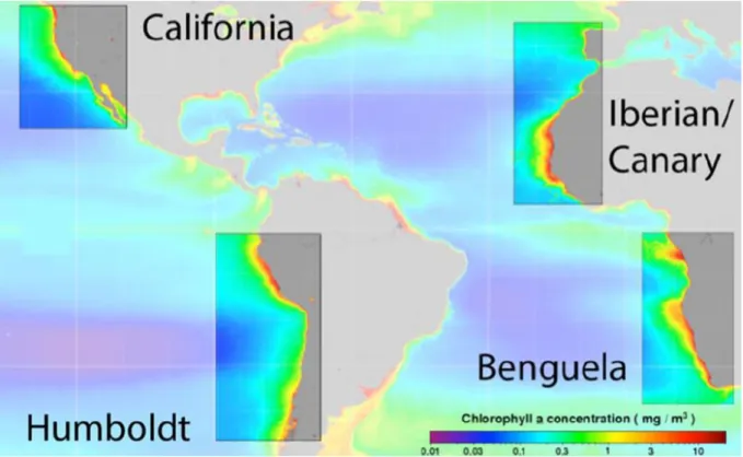
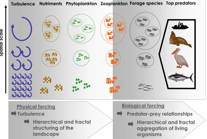
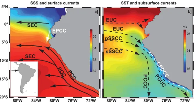
Figure 1.1. EBUS localization and their chlorophyll-a annual average concentrations. Source Bakun et al. 2015. ………...……5 Figure 1.2. Fish catch versus primary productivity for the four main eastern boundary coastal upwelling ecosystems for the years 1998–2005. It was assumed that the reported fish catches (Fish and Agriculture Organization, FAO) were made within 100 km from the coast. The catches were then normalized by area. Primary productivity was estimated from satellite remote sensing of chlorophyll and the Behrenfeld and Falkowski (1997) model. Even during the El Niño year of 1998 Peru fish catch still exceeded that from the other areas by several fold. Is Peru exceedingly efficient in the transfer of primary production to fish or are Benguela and Northwest Africa exceedingly inefficient? Source Chavez et al. 2008. ………..……6 Figure 1.3. First ‘‘ecosystem-based” diagram for the northern Humboldt Current System developed when seabirds were the focus of management Source Chavez 2008 and reprint from Vogt 1948. ………..7 Figure 1.4. Schematic representation of the concept of bottom-up transfer of behavior and spatial structuring. …..………8 Figure 1.5. Sea surface properties and oceanic circulation scheme of the NHCS. Sea-surface salinity (SSS, color shading) and surface circulation, right panel. Sea-surface temperature (SST, color shading in °C) and subsurface circulation, left panel. The newly defined Ecuador-Peru Coastal Current (EPCC) and Chile-Peru Deep Coastal Current (CPDCC) are indicated by white arrows. Surface currents. SEC: South Equatorial Current; EPCC: Ecuador-Peru Coastal Current; POC: Peru Oceanic Current; PCC: Peru Coastal Current. Subsurface currents. EUC: Equatorial Undercurrent; pSSCC: primary (northern branch) Southern Subsurface Countercurrent; sSSCC: secondary (southern branch) Southern Subsurface Countercurrent; PCCC: Peru-Chile Countercurrent; PCUC: Peru-Chile Undercurrent; CPDCC: Chile- Peru Deep Coastal Current. Source Chaigneau et al 2013. ….………..10 Figure 1.6. Schematic distribution of characteristic surface water masses: a) latitudinal distribution of surface water masses along the Peruvian Coast (Ayon et al 2008), vertical distribution of water mass based on b) Salinity and c) temperature from the fourth section of a glider deployment (at 14 ° S). Source Pietri et al 2014. Cold coastal waters (CCW), the subtropical surface waters (STSW), the equatorial surface waters (ESW), and the tropical surface waters (TSW), the eastern south Pacific intermediate water (ESPIW) and the Antarctic intermediate water (AAIW). …..………...11
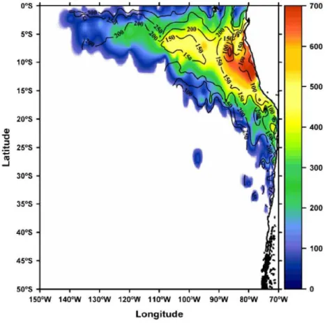
ii Figure 1.7. Oxygen Minimum Zone (OMZ, < 20μmolkg-1
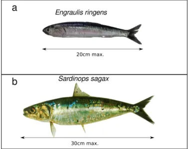
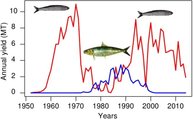
) thickness (m) in the south-eastern Pacific. Thickness is colour-coded according to the color bar on the right-hand side of the figure. The upper boundary of the OMZ is shown in black contour lines with 50 m intervals. Source Fuenzalida et al. 2009. …..……….12 Figure 1.8. Simplified food web of NHCS, centered on euphausiid Euphausia mucronata during a period of high biomass of anchovy Engraulis ringens. Thickness of the arrows indicates the relative flow of biomass between components. Souce Antezana 2010. ……….14 Figure 1.9. Peruvian (a) anchovy and (b) sardine. …..………..……16 Figure 1.10. Most common seabird species that depends on forage fish included a) Cushuri (P.
olivaceous), b) the Guanay cormorant (P. bougainvillii), c) the Red-legged cormorant (P. gaimardi), d) Peruvian booby (S. variegata), e) the Blue-footed booby (S. nebouxii), f) the
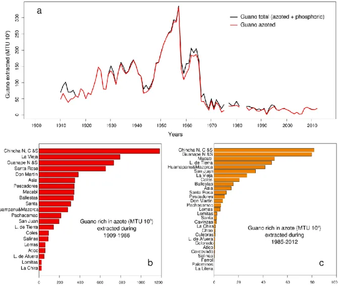
Humboldt penguin (Spheniscus humboldti), g) the Peruvian pelican (Pelecanus thagus), h) and the Inca tern (Sterna inca). The i) Kelp gull (Larus dominicanus) is a common species that feed on eggs, chicks and regurgitates of guano seabirds breeding in sympatry. ………..19 Figure 1.11. Main marine mammal species occurring in the NHCS. Source Majluf 1989. …….21 Figure 1.12. Purse-seiners used to catch anchovy, a) “industrial” purse seiner with a steel hull and b) “artisanal” purse-seiner with a wooden hull. …..………...22 Figure 1.13. Time series of annual yield (MT) of anchovy and sardine in the NHCS. Source of data, IMARPE. …..………..………..……23 Figure 1.14. Abundances of seabirds (cormorants, boobies and pelicans) from 1952 to 2014, and catch of anchovy and sardine. Years when strong El Niño events occurred are marked by orange bars. Data source AGRORURAL and IMARPE. …..………...25 Figure 1.15. Map of the main seabird colonies during 1956. Source: 48 Memoria del Directorio de la Compania Administradora de Guano. …..………...26 Figure 1.16. a) Guano extracted per year during the last century in the main seabird colonies (Data source AGRORURAL), b) Guano extracted by nesting site from 1909-1966, period of large abundance of anchovy and under the CAG administration and c) guano extracted during 1985-2012, period of less abundance and posterior recuperation of anchovy but not of seabirds. Data source for b and c were Cushman 2003 and AGRORURAL pers.com. …..………...27 Figure 1.17. Map of the main seabird colonies during 2009, when the National Reserve of Guano Island, Islets and Headland was created. Source AGRORURAL. …..………..…...28 Figure 1.18. Stommel’s diagram showing how population or “biomass variability” is linked to the oceanic process in time-space scales. It represented a conceptual model of the time-space
iii scale of zooplankton biomass variability and the factors contributing to this scales. I, J, K, are bands centered about thousands and tens of kilometers in space scale with time variations between weeks and geological time scales. Source Haury et al. 1978. …..………...…...29 Figure 1.19. Fish debris deposition rates off Pisco, Peru for A) Anchovy vertebrate fluxes (# vertebrae.103y-1cm-2) and B) Sardine scale fluxes (# scales.103y-1cm-2). Highlighted areas indicate the Current Warm Period (CWP from ~1900 to the present), Little Ice Age (LIA, from 1500 to 1850AD), the Medieval Climate Anomaly (MCA, from 900 to 1350AD) and the Dark Ages Cold Period (500 – 900 AD). Source Salvatecci 2013. …..……….…...30 Figure 1.20. Conceptual model of decadal changes in anchovy and sardine populations in the southeastern tropical Pacific. Schematic representation of a) the temporal changes in abundance of large plankton and anchovy (blue) and small plankton and sardine (orange) during 1960-2010. b) Energetic costs of feeding on dominant plankton size-spectra for anchovy and sardine according to the scenarios from a. c). Schematic of the available habitat for anchovy (blue shaded area) and sardine (red shaded area). Source, Bertrand et al. 2011. …..……….…...32 Figure 1.21. Schematic representation of a) La Niña, b) Normal conditions and c) El Niño conditions in the Pacific Ocean. Source: NOAA / PMEL / TAO Project Office. ……….……...33 Figure 1.22. Graphical representation of El Niño regions based on sea surface temperature data collected in the eastern and central tropical Pacific Ocean. Source:
http://www.cpc.ncep.noaa.gov/products/analysis_monitoring/ensostuff/nino_regions.shtml. …34
Figure 1.23. Time series of the SST anomalies in the El Niño 1+2 are. Red portions of the line refer to EN conditions according to Trenberth 1997 and portions in blue refer to LN conditions according to Trasmonte and Silva 2008. Source of time series:
http://www.cpc.ncep.noaa.gov/data/indices/ersst3b.nino.mth.81-10. …..………....34
Figure 1.24. Guanay cormorant, a) adult in ventral view, b) adult in dorsal view. …..…….…...38 Figure 1.25. Peruvian booby, a) adult in ventral view, b) adult in dorsal view and c) young of Peruvian booby. …..………...…...39 Figure 1.26. Peruvian pelican, a) adult in dorsal view, b) adult in ventral view. …..…………...40 Figure 1.27. Monthly distance travelled in miles by a) Guanay cormorant and b) Peruvian booby. Data source Jordan 1958; Jordan & Cabrera 1960. …..………....41 Figure 1.28. Guanay cormorant, a a) recently emerged chick b) and chicks of 2-3 weeks. Peruvian booby, adults with two chicks of 2-3 weeks. Peruvian pelican, d) adults with several chicks in a “crèche”. …..………...42
iv Figure 1.29. Comparison of maximum sustained working level of parent birds tending nestlings with the working level of heavy labor by human standards. Maximum sustained working level is expressed as metabolizable energy per day (DME). Examples are of Asia atus, Delichan urbica,
Sturnus vulgaris, Larus glaucescens and Streptapelia risaria. Source Drent & Daan 1980. …...46
Figure 1.30. Hypothetical relationship between food supply, date of laying eggs and date of young becoming independent in two species, (a and b). The black curves show the level of food abundance against the food required for body maintenance (green) and the food required for forming eggs (red). Depending on the species, the time required from forming, laying and incubate eggs (X) varies and the amount of food availability affects the capacity to raise the young to the point of independence (Y). Redrawn from Perrins 1970. …..………...……...46 Figure 1.31. Warmer air temperature is proximate factor used by Great tit (Parus major) for triggering the onset of egg laying. The ultimate factor is the availability of caterpillar when chicks are reared and when birds’ energetic demands are highest. Source Durant et al. 2007. ...48 Figure 1.32. Schematic representation of the neuroendocrine cascade controlling expression of sexual behavior. Redrawn from Hau et al. 2001. …..………...48 Figure 1.33. Diagram showing how many times each month occurs in the records of egg-seasons in each 10° of latitude. Graphic was done from date of egg- laying dates from 254 species of Old World birds according with its latitudinal location. Source Baker 1939. …..………...49 Figure 1.34. Model proposed by Wingfield et al. (1992) about the theoretical relationships between the environmental information factor (Ie) and the environmental information needed to optimize the timing of breeding, with the relative contribution of two types of environmental information (initial predictive information and supplementary information). As Ie tends towards zero, the individual respond only to predictive information. When Ie increases, supplementary information becomes important. When Ie is very high supplementary information may predominate. Source Wingfield et al. 1992. …..………...50 Figure 1.35. Example of an original field data sheet of the seabird census for Mazorca Island on September 2007. Information about occupied patches by species, age and reproductive status were recorded. Surface occupancy was converted to abundances by multiplying surface occupancy by a species-specific conversion factor of density (number of nests/individuals by m2). Some labels were translated for better understanding. …..……….……...52 Figure 1.36. Different types of metapopulation. Filled circles represent occupied habitat patches; empty circles represent vacant habitat patches; dotted lines represent boundaries of local populations; arrows represent dispersal. a) Classic boundaries of Levins; b) mainland- island; c) patchy population; d) nonequilibrium metapopulation; e) intermediate case combining features of (a), (b), (c), and (d). Source Harrison & Taylor 1997. …..……….………...54
v Figure 1.37. Schema of the estimation of parameters in multiseason occupancy models. Ψ is the initial occupancy (ψ=1, or 1-ψ=0), then in the next seasons (S1, S2 and S3) extinction (Pr(h=10) =ε) or colonization (Pr(h=01)=γ) parameter are estimated. …..……….…...55 Figure 2.1. Map figuring the 31 breeding sites of guano producing seabirds (Guanay cormorant, Peruvian booby and Peruvian pelican) monitored by AGRORURAL along the coast of Peru. ..63 Figure 2.2. Estimates of monthly probabilities of breeding onset for (a) cormorants (solid black line), (b) boobies (dashed line) and (c) pelicans (dotted thick line) related to oceanographic conditions (PC1, dashed lines with dots), standardized anchovy abundance (sA, solid white lines) and standardized anchovy body condition (BCF, dotted thin lines). Shaded areas correspond to 95% confidence intervals. Lines of breeding onset, oceanographic conditions and anchovy body conditions were smoothed with a loess model with 0.45 of span. Effects of nesting habitat covariates on breeding onset probability. …..………...68 Figure2.3. Modeled probabilities of breeding onset as a function of (a) oceanographic conditions (PC1 standardized), (b) the standardized regional anchovy abundance (sA), and (c) standardized anchovy body condition factor (BCF) for boobies (dashed lines) and pelicans (dotted thick lines). The functional relationships were obtained from the selected models for each species (P < 0.005 and highest R²). Shaded areas represent = 95% confidence intervals. …..……….………...71 Figure 2.4. Schematic representation of the onset (dark gray) and termination (i.e. fledging; light gray) of breeding seasons for cormorants, boobies and pelicans related to seasonal variability in environmental conditions. In the section of seasonal variability in environmental condition dark gray area indicates maximum and light gray area minimum values; ‘x’ indicates the lack of data. ………73 Figure 3.1. Functional Principal components of SST and Chlorophyll. Loadings (a and c) were represented on the left and the bivariate plot of scores of each colony for FPC1 and FPC2 (b and d) were represented on the right. Extended names of the nesting sites are described in Appendix A. …..………..………...88 Figure 3.2. Functional Principal components of Upwelling index and Depth of oxycline. Loadings (a and c) were represented on the left and the bivariate plot of scores of each colony for FPC1 and FPC2 (b and d) were represented on the right. Extended names of the nesting sites are described in Appendix A. …..………...89 Figure 3.3. Functional Principal components of onset and occupancy of cormorant. Loadings of timing and magnitude of onset of breeding of cormorant were represented on the left (a and c) and the bivariate plot of scores of each colony for FPC1 and FPC2 (b and d) were represented on the right. Extended names of the nesting sites are described in Appendix A. …..………….…...93
vi Figure 3.4. Functional Principal components of onset and occupancy of booby. Loadings of timing and magnitude of onset of breeding of pelican were represented on the left (a and c) and the bivariate plot of scores of each colony for FPC1 and FPC2 (b and d) were represented on the right. Extended names of the nesting sites are described in Appendix A. …..…………...……...94 Figure 3.5. Functional Principal components of onset and occupancy of pelican. Loadings of timing and magnitude of onset of breeding of pelican were represented on the left (a and c) and the bivariate plot of scores of each colony for FPC1 and FPC2 (b and d) were represented on the right. Extended names of the nesting sites are described in Appendix A. …..………...………...96 Figure 3.6. Schematic representation of the variability of seasonal breeding and covariates that explained that variation. …..………...………...98 Figure. 4.1. Seasonality of oxycline depth (a), sea surface temperature (b), chlorophyll (c), biomass of anchovy (d) and monthly fishing pressure (e) in the Peruvian coast during the periods of 1952-1968 (solid lines), 1977-1990 (dashed lines) and 2000-2014 (dotted lines). Shaded areas represented the 95% and 5% confidence levels of sample mean. …..………...……….109 Figure4.2. Monthly average estimates of probability of onset of breeding during the periods of 1952-1968 (solid lines), 1977-1990 (dashed lines) and 2003-2014 (dotted lines) for cormorants (a, b and c), boobies (d, e and f) and pelicans (g, h and i). Seasonalities of oxycline depth (dashed lines with dots) and biomass of anchovy (dotted thin lines) are also represented for the three periods and its respective axes are at the right of plots. Shaded areas represented the95% and 5% of the posterior distribution of monthly probability of onset of breeding. Breeding onset probability, oxycline depth and biomass of anchovy were smoothed with a loess model with 0.45 of span. …..……….112 Figure4.3. Monthly average estimates of probability of occupancy of breeders for cormorants (a), boobies (b) and pelicans (c) during 1952-1968 (solid lines), 1977-1990 (dashed lines) and 2003-2014 (dotted lines). Shaded areas represented the 95% and 5% of the posterior distribution of monthly probability of onset of breeding. Breeding onset probability lines were smoothed with a loess model with 0.45 of span. ..……….113 Figure 5.1. Schematic representation of the relationships between seabird demographic traits and the marine environment. The breeding frequency is highlighted in red font because is the central topic of these thesis. Source, Weimerskirch 2001. ……….……...124 Figure 5.2. Example of the state and observation process of a marked individual over time for the Cormack Jolly Seber model. The sequence of true states in this individual is z = [1, 1, 1, 1 ,1, 0, 0],and the observed capture-history is y = [1, 1, 0, 1, 0, 0, 0].Source Kéry & Schaub 2012. ……….……..129 Figure 5.3. Graphical representation of an integrated population model (IPM) within a Bayesian approach. Small squares represent the data, circles the parameters (blue: target parameters, green: nuisance parameters), large squares the individual submodels, and arrows the flux of information. Circles appearing in two submodels indicate that they are informed from two data
vii sources. IPM model represent three data types: i) count data where y is the observed data, N is the true abundance and 𝜎2𝑦 is the observational error; ii) productivity data where J is the number of nestling recorded and R is the annual number of surveyed broods; and iii) capture-recapture data where m is the number of released individuals never captured, Sjuv and Sad are survival of
juveniles and adults respectively and p is the observational error. Source Kéry & Schaub 2012. ..………...……….130 FIG A1. Monthly percentage of seabirds observed incubating eggs for pelicans (blue line), boobies (red line), and cormorants (black line). Monthly percentage of anchovy abundance near the nesting place is also shown (dashed green line). Redrawn from Vogt (1942). ……….158 FIG. C1. Example of an original field data sheet of the seabird census for Mazorca Island on September 2007. Information about occupied patches by species, age and reproductive status were recorded. Surface occupancy was converted to abundances by multiplying surface occupancy by a species-specific conversion factor of density by m2. Some labels were translated for better understanding. ..………160 FIG. D1. Colony size frequency distribution for the three species of cormorants, boobies and pelicans. Histograms correspond to the raw abundance data (left column), the abundance data without breeder absences (central column), the abundance data without breeder absences once log10-transformed (right column). ..………164 FIG. E1. Monthly climatology profiles of (a) sea-surface temperature (SST), (b) chlorophyll (Chlo), (c) upwelling index (UI), (d) oxycline depth (Z2ml l-1) and (e) dissolved oxygen concentration (DO) at the surface. The boxplots were constructed from the site-specific climatology profiles built over an area covering a radius of 100 km around each breeding site. Periods encompassed 1999-2009 for SST, Chlo and UI and 1960-2010 for DO and Z2ml l-1. ………..166 FIG. E2. Results from a principal component analysis of oceanographic covariates. The x-axis represents the first principal component (89.1% of the variance) and the y-axis represents the second principal component (7.3% variance). ………167 FIG. F1. An example of a systematic parallel cross-shore transects used on a Peruvian acoustic anchovy survey from November to December of 2006 involving one vessel research. Red points indicate seabird nesting sites and the green line indicates the first 40 km offshore limit used to calculate montly climatologies of abundance and horizontal distribution of anchovy. ………..168 FIG. F2. Monthly variations of anchovy abundance (a) sA, (b) sA+ and (c) index of space occupation (ISO). The boxplots were constructed from the monthly variations of the metrics between 6° and 14°S over the period 1999-2011. ………..171
viii FIG. G1. Monthly variations of anchovy physiological condition metrics (a) body condition factor, BCF; and (b) Gonado-somatic index: GSI. Boxplots were constructed from monthly variations of the metrics between the 6° to 14°S over the 2000-2012 period. ………...172 FIG. I1. Estimates of monthly probabilities of breeding onset (green solid line) and breeding termination (orange solid line) for (a) cormorants, (b) boobies and (c) pelicans in the Northern Humboldt Current System over 10 years. Shaded areas correspond to 95% confidence intervals. ………..177 Figure A1. Schematic map of the localization of the main colonies of Guanay cormorant, Peruvian booby and Peruvian pelican. ………186 Figure A2. Main ports of landings of anchovy, in gray letters nesting colonies near the ports. ………..187 Figure A3. Map of localization of nesting colonies for the three seabirds. Colony size is represented by colors. Largest colonies are represented in red (100 000 – 250 000 for cormorant and booby and 10 000 – 50 000 for pelican) and smallest colonies in yellow (<10 000 for cormorant and booby and <5 000 for pelican). In the left panel longitude is suppressed and latitudinal effect on colony size is showed for the thee species. ………188 Figure A4. Correlation matrix of Site-specific, abundance of seabirds and fisheries variables. ………..189 Figure C1. Schema of procedure in Random forest. ………...193 Figure C2.Schema of PIMP procedure for correct categorical variable bias importance and select only significant important variables. ………...194 Figure D1. Mean (red line) and outliers (green lines) of onset and occupancy for cormorant, booby and pelican. ………..195 Figure D2. Mean (red lines) .and outliers (green lines) of oceanographic conditions. ………...196 Figure E1. The right plot sorts the variables by importance to explain the FPC1 of the onset of breeding of cormorant. Variables were geographic (Lat, S, I/H), scores of functional components of oceanographic covariates (SSTFPC, ChloFPC, Z2mlFPC, UIFPC), fisheries pressure (LA100, DNP). On the left, there are represented the partial plot of the significant variables.social variables (AbC). The important significant variables fall above the red line (p>0.05). ……….197 Figure E2. The right plot sorts the variables by importance to explain the FPC1 and FPC2 of the occupancy of breeders of cormorant. Variables were geographic (Lat, S, I/H), scores of functional components of oceanographic covariates (SSTFPC, ChloFPC, Z2mlFPC, UIFPC), fisheries pressure (LA100, DNP). On the left, there are represented the partial plot of the
ix significant variables.social variables (AbC). The important significant variables fall above the red line (p>0.05). ………...198 Figure E3. The right plot sorts the variables by importance to explain the FPC1 and FPC2 of the onset of breeding of booby. Variables were geographic (Lat, S, I/H), scores of functional components of oceanographic covariates (SSTFPC, ChloFPC, Z2mlFPC, UIFPC), fisheries pressure (LA100, DNP). On the left, there are represented the partial plot of the significant variables.social variables (AbC). The important significant variables fall above the red line (p>0.05). ……… .199 Figure E4. The right plot sorts the variables by importance to explain the FPC1 and FPC2 of the occupancy of breeders of booby. Variables were geographic (Lat, S, I/H), scores of functional components of oceanographic covariates (SSTFPC, ChloFPC, Z2mlFPC, UIFPC), fisheries pressure (LA100, DNP). On the left, there are represented the partial plot of the significant variables.social variables (AbC). The important significant variables fall above the red line (p>0.05). ………..200 Figure E5. The right plot sorts the variables by importance to explain the FPC1 of the onset of breeding of pelican. Variables were geographic (Lat, S, I/H), scores of functional components of oceanographic covariates (SSTFPC, ChloFPC, Z2mlFPC, UIFPC), fisheries pressure (LA100, DNP). On the left, there are represented the partial plot of the significant variables.social variables (AbC). The important significant variables fall above the red line (p>0.05). ……….201 Figure E6. The right plot sorts the variables by importance to explain the FPC1 and FPC2 of the occupancy of breeders of pelican. Variables were geographic (Lat, S, I/H), scores of functional components of oceanographic covariates (SSTFPC, ChloFPC, Z2mlFPC, UIFPC), fisheries pressure (LA100, DNP). On the left, there are represented the partial plot of the significant variables.social variables (AbC). The important significant variables fall above the red line (p>0.05). ………..202 Figure S1. Barplots of data available among the years for a) 𝑍2𝑚𝑙𝑙−1,b)Chlorophyll and c)SST. Data are classified by periods: green 1952-1968, red 1977-1990 and blue 2000-2012. For the most recent period we use oceanographic data since 2000 because it corresponded to the same regime and allowed us to build a stronger climatology.. ………..…………205 Figure S2. Barplots of data available of a) SST, b) 𝑍2𝑚𝑙𝑙−1 and c) Chlorophyll for each month during the periods: 1952-1968 (green), 1977-1990 (red) and 2003-2014 (blue). ………....205 Figure S3. Anomalies of sea surface temperature of the zone El Nino 1+2 since 1950 to 2014. Base climatology to analyze the anomalies was built from 1981-2010 (http://www.cpc.ncep.noaa.gov/data/indices/ersst3b.nino.mth.81-10.ascii). Continuous anomalies for more than 5 months and higher than 0.4°C are identified as El Nino events (Trenberth 1997,
x red lines) and continuous anomalies for more than 5 months and lower than -1.0°C are identified as La Nina (Trasmonte & Silva 2008, blue lines). ………..206 Figure S4. Estimates of monthly probabilities of onset of breeding (green solid line) and termination of breeding (orange solid line) at the breeding sites for (a) cormorants, (b) boobies and (c) pelicans in the Northern Humboldt Current System for the period 2003-2012 from Passuni et al. (2015). Shaded areas correspond to 95% confidence intervals. ………...208 Figure S5. Output of a-c) onset, d-f) termination, and g-i) occupancy of breeding for Guanay cormorants for the periods 1952-1968, 1977-1990 and 2003-2014 with different hyperparameters: Uniform (red boxes), Jeffrey (green boxes) and Informative (blue boxes). 211 Figure S6. Output of a-c) onset, d-f) termination, and g-i) occupancy of breeding for Peruvian boobies for the periods 1952-1968, 1977-1990 and 2003-2014 with different hyperparameters: Uniform (red boxes), Jeffrey (green boxes) and Informative (blue boxes). ………...212 Figure S7. Output of a-c) onset, d-f) termination, and g-i) occupancy of breeding for Peruvian pelicans for the periods 1952-1968, 1977-1990 and 2003-2014 with different hyperparameters: Uniform (red boxes), Jeffrey (green boxes) and Informative (blue boxes). ………213
xi
List of Tables
Table 1. 1. List of the seabird species observed near the coast in NHCS. References: 1 (Murphy 1936), 2 (Tovar Serpa 1969), 3 (Figueroa & Stucchi 2008), 4 (Stucchi et al. 2011), 5(Reserva Nacional Sistema de Islas 2009), 6 (Duffy 1981). …..………...……….…….17 Table 1.2. Approximate duration of the main breeding stages (in days) from pre-laying attendance to the independence of fledglings for cormorants, boobies and pelicans. Pre-laying attendance includes forming a couple and building a nest, post-fledging includes rearing of youngs by adults after fledging. 1 (Nelson 2005 mainly from Galarza Ninaya 1968), 2 (Schreiber & Burger 2002), 3 (Tovar Serpa & Cabrera Quiroz 2005). …..………...………43 Table 2.1. Summary of selected models relating oceanographic conditions (PC1), anchovy regional and local abundance (sA and sA+), anchovy body condition (BCF) and the Gonado-somatic index (GSI) to the probabilities onset of breeding (γ) for cormorant, booby and pelican. Monthly termination of breeding [ε(m)] were not changed between models. Oceanographic conditions, body condition and the Gonado-somatic index were lagged of one month. Notes: The slope (β) ± SE indicates the shape of the relationship between covariates and onset of breeding. The F statistic of ANODEV (noted Fcst/cov/t) and its associated p-value (P) test the covariate
effect on onset of breeding, while R2 provides a measure of the magnitude of the effect. I/H is the geographical effect that in case of pelican changes to DC. ……….70 Table 3.1. Results of FPCA for onset and occupancy for each seabird and oceanographic conditions. …..……….………90 Table 3.2. Results of regression models performed with random forest. Regression models were done between timing and magnitude of onset and occupancy of breeders for the three species as dependent variables and site-specific, oceanographic and prey covariates. Variables presented were significant (P-value>0.05, FDR>0.1). …..……….……….…92 Table 4.1. Models of onset (γ) of breeding related to the depth of oxycline (Z2ml l−1), SST and Chlo. Mean (µ) and standard deviation (sd) of intercept (β0) and slope (β1). The parameter f represents the
proportion of posterior with the same sign as the mean. We consider as significant f > 97.5 and the mean and f are indicated in bold. …..………..……….…………115 Table 4.2. Models of onset (γ) of breeding related to the anchovy biomass and fishing pressure. Mean (µ) and standard deviation (sd) of intercept (β0) and slope (β1). The parameter f represents the proportion of
posterior with the same sign as the mean. We consider significant as f > 97.5 and the mean and f are indicated in bold. …..………..………...……117 Table B1. Approximate duration of the main breeding stages (in days) from pre-laying attendance to the independence of fledglings for cormorants, boobies and pelicans. Information is based on Schreiber (2002), Nelson (2005), Tovar Serpa and Cabrera Quiroz (2005). Pre-laying attendance includes forming a couple and building a nest, post-fledging includes rearing of young by adults after fledging. …………159
xii TABLE D1. Minimum, mean and maximum colonies size (number of individuals) for the Guanay cormorant, the Peruvian booby and the Peruvian pelican. ………162 TABLE D2. Percentage of nesting sites occupied in every month, averaged over all years for the Guanay cormorant, the Peruvian booby and the Peruvian pelican. ………163 TABLE F1. List of cruises which data have been used to compute monthly climatologies of abundance and horizontal distribution of anchovy. ………169 TABLE I1. Testing for Markovian processes in probabilities of breeding onset (γ) and breeding termination (ε) in cormorants, boobies and pelicans. The AIC (Akaike Information Criterion), ΔAIC (difference in Akaike Information Criterion), w (Akaike weight) and np (number of parameters of the model) are given. ………...175 TABLE I2. Modelling time variation of probabilities of breeding onset (γ) and termination (ε) in cormorants, boobies and pelicans. AIC (Akaike Information Criteria), ΔAIC (difference in Akaike Information Criteria), w (Akaike weight) and np (number of parameters of the model). ………176 TABLE I3. Modelling the effects of geographical covariates on the probabilities of breeding onset (γ) and breeding termination (ε) for cormorants, boobies and pelicans. AIC (Akaike Information Criteria), ΔAIC (difference in Akaike Information Criteria), w (Akaike weight) and np (number of parameters of the model). ………..178 TABLE I4. Testing for the effects of oceanographic covariates on the probabilities of breeding onset (γ) and breeding termination (ε) for cormorants, boobies and pelicans using ANODEV. Oceanographic covariates are synthesized by the first component (PC1) of a principal component analysis (see Appendix M). Dev is the deviance of the model, the F statistic of ANODEV (noted Fcst/cov/t) and its associated value (P) test the effect of the oceanographic covariate on monthly onset and termination probabilities, while R2 provides a measure of the magnitude effect. I/H is the geographical effect that, for pelicans, changes to DC. The slope (β) ± SE indicates the shape of the relationship between γ or ε and PC1 taken with a one to three-month lag. ………..179 TABLE I5. Testing for the effects of global (sA) and local (sA+) anchovy abundance and distribution (ISO) on the probabilities of breeding onset and breeding termination for cormorants, boobies and pelicans using ANODEV. Dev is the deviance of the model, the F statistic of ANODEV (noted Fcst/cov/t) and its associated value (P) test the effect of prey abundance and distribution on monthly onset and termination probabilities, while R2 provides a measure of the magnitude effect. I/H is the geographical effect that, for pelicans, pelican changes to DC. The slope (β) ± SE indicates the shape of the relationship between γ or ε and anchovy abundance and distribution……….180 TABLE I6. Testing for the effects of anchovy physiological condition (BCF and GSI) on the probabilities of breeding onset and termination by cormorants, boobies and pelicans using ANODEV. Dev is the deviance of the model, the F statistic of ANODEV (noted Fcst/cov/t) and its associated value (P) test the effect of anchovy condition on monthly onset and termination probabilities, while R2 provides a measure of the magnitude effect. I/H is the geographical effect that, for pelicans, changes to DC. The slope (β) ± SE indicates the shape of the relationship between γ or ε and anchovy physiological condition, taken with a one to three-month lag. ………...181
xiii Table A1. Main nesting colonies of cormorants, its geographic characteristics and average size total and for each species. ………184 Table S1. Number of months consigned for each period of data time series. In parenthesis the years were data was missing for each month……….. 204 Table S2. Mean (µ), variance (σ2) and enlarged variance (σ2 used) of the onset and termination of breeding for the cormorants, boobies and pelicans from 2003-2012 of 31 breeding sites in the Peruvian coast obtained from Passuni et al. (2015). Enlarged variance (maximum for onset 0.01 and termination 0.02), the hyperparameters α and β of the beta distribution were calculated for the three species. β and α hyperparameters for informative prior distribution were calculated from mean and enlarged variance. .208 Table S3. Comparison of deviance information criterion (DIC) between the three priors used to model probabilities of occupancy, onset of breeding and termination of breeding: Uniform, Jeffrey and informative for the three species and the three periods. Comparison between models was only done when the dependent variable did not change, i.e. by rows. The lower DIC with a difference of 5 was selected in bold. ………...210 Table S4. Identifiability of onset (τ_γ), termination (τ_ε) and occupancy (τ_ψ) of breeders for the three seabirds during the three periods analyzed. Values indicated with * were not considered as not identifiable because >70% of overlap between the prior and posterior distribution. 70% were the average of overlap for the probabilities of termination of breeding. ………...214 Table S5.. Mean and standard deviation of onset (γ) and occupancy (ψ) probabilities, Kruskal-Wallis tests and correlation tests for the three periods and the three species. Dunn post-hoc tests were performed when Kruskal-Wallis tests were significant. Significant differences between periods (P < 0.05) are highlighted in bold (mean and standard deviation). For correlation tests with a Pearson coefficient (Z) significant results are in bold (P < 0.05). ………...216 Table S6. Life history traits of cormorants, boobies and pelicans. 1, 2 and 3 are approximate measures corresponding to family members or similar species. Information is based on Nelson 2005, Duffy and Ricklefs 1981, Nelson 1977. ……….217
xiv
Résumé executif
Introduction
Le Système Nord du Courant de Humboldt (SNCH) est le lieu d’une forte activité biologique due à un upwelling côtier intense. Il abrite l’une des plus grandes populations de petits poissons pélagiques, l’anchois du Pérou, et la plus grande pêcherie monospécifique au monde. Ces grandes abondances d’anchois sont aussi à la base de l’alimentation des principaux prédateurs supérieurs comme les oiseaux et mammifères marins. Le SNCH héberge de grandes, quoique variables, populations d’oiseaux, composées entre autres de trois espèces sympatriques productrices de guano: le cormoran guanay (Phalacrocorax
bougainvillii), le fou péruvien (Sula variegata) et le pélican péruvien (Pelecanus thagus), qui se
nourrissent principalement d’anchois.
Le SNCH connaît une très forte variabilité environnementale, à une grande variété d’échelles spatio-temporelles. Dans sa composante spatiale, il y a des différences remarquables entre les eaux côtières et les eaux au large de la côte. Les eaux côtières sont froides, avec une forte production près de la surface qui épuise l’oxygène rapidement dans la colonne d’eau. Les eaux du large sont plus chaudes, moins productives et plus oxygénées. En conséquence, l’intensité d’upwelling et l’oxygène disponible sont des processus très structurants des habitats des organismes vivants dans cet écosystème. Cette structuration est soumise à une grande variabilité temporelle aux échelles saisonnières, interannuelles, décennales, centennales et millénaires. Ces fluctuations peuvent avoir des répercussions importantes sur la distribution et l’histoire de vie des espèces, comme la reproduction notamment.
En sus de la variabilité climatique naturelle, le système et aussi soumis à une forte pression anthropique. Concernant les oiseaux par exemple, il existe des évidences qu’avant la découverte de l'Amérique, les populations locales utilisaient leurs excréments (« guano ») pour améliorer les cultures. Au XIXème siècle, la redécouverte au niveau international des propriétés du guano crée une industrie d’exploitation très importante pour l’économie du pays. L’exploitation intensive conduisit à un rapide épuisement des stocks et un défaut de renouvellement du guano. Suite à l’effondrement de l’exploitation de guano, des efforts de conservation et d’aménagement de l’habitat des oiseaux furent déployés. Ces efforts, en conjonction avec une fluctuation climatique favorisant l’anchois, résultèrent en une rapide augmentation des populations d’oiseaux et la récupération de l’industrie d’exploitation de guano. Cependant, à partir des années 1950, la façon dont les humains exploitent l’écosystème côtier connut un changement radical. Le développement rapide d’une pêcherie industrielle à l’anchois convertit les humains de commensaux des oiseaux, au travers de l’exploitation du guano, à des compétiteurs directs pour l’accès au poisson fourrage. Cette forte pression compétitive associée à des conditions climatiques adverses comme les évènements El Niño, produisit des fluctuations drastiques du nombre d’oiseaux producteurs de guano. Aujourd'hui, les populations d’oiseaux producteurs de guano sont aussi devenues source d’attraction touristique. L’Etat péruvien se préoccupe donc de la santé de ces populations, non seulement vis-à-vis des effets d’évènements ponctuels comme El Niño qui ont été relativement bien documentés, mais aussi et
xv surtout vis-à-vis de l’impact global des variabilités d’origine climatique et anthropogénique qui sont moins bien connues.
La reproduction est un processus clé du cycle de vie, susceptible d’être affecté en premier lieu par les effets du changement climatique et des fluctuations environnementales. La reproduction chez les vertébrés est l’une des phases du cycle de vie demandant les plus forts apports énergétiques. Pour cette raison, la reproduction est généralement saisonnière et synchronisée avec la période où l’abondance de ressources est maximale dans l’écosystème. L’intégration des fluctuations saisonnières de signaux environnementaux comme la lumière, la température ou la pluie est utilisée pour anticiper la période où les ressources seront les plus abondantes. On sait d’autre part que le changement climatique risque d’affecter ces cycles saisonniers et donc de remettre en question la valeur de ces indices environnementaux pour le déclenchement de la reproduction. Des risques de décalage ou « mismatch » entre la reproduction et l’abondance des ressources peuvent apparaître (Visser, Both & Lambrechts 2004) et entraîner des échecs de reproduction à court terme, et des diminutions de population à long terme (Both
et al. 2006).
Dans le SNCH, le cycle saisonnier est décrit comme modéré, avec une grande influence de l’intensité de l’upwelling, de la lumière utilisée pour la photosynthèse et de la profondeur de l’oxycline. En hiver, on observe un intense upwelling et une faible profondeur de l’oxycline mais moins de lumière ce qui limite la production primaire. Au printemps, il y a moins d’intensité d’upwelling, mais plus de lumière et moins de stratification dans la colonne d’eau ce qui permet une production supérieure. Cette production perdure jusque la fin de l’été (Echevin et al. 2008). Si la saisonnalité des conditions océanographique est bien décrite, on dispose de peu d’informations sur le cycle saisonnier des organismes vivants comme les oiseaux marins dans le SNCH. Dans ce travail, nous examinons les fluctuations de ces trois populations d’oiseaux marins, en nous concentrant sur le cycle saisonnier de leur reproduction, pour aborder les questions suivantes: Les oiseaux producteurs du guano ont-ils des cycles saisonniers? Dans quelle mesure les saisonnalités de reproduction diffèrent-elles entre espèces ? Dans quelle mesure sont-elles plastiques dans le temps et dans l’espace ? Qu’est ce qui, des conditions environnementales et des activités anthropogéniques, affecte le plus la reproduction des oiseaux marins ?
La thèse est organisée en un chapitre introductif (chapitre 1) qui fournit une vue d’ensemble sur le fonctionnement du SNCH et trois chapitres centraux (chapitres II, III, IV) prenant la forme de trois publications.
Dans le chapitre II, on analyse la saisonnalité de la reproduction des oiseaux, les différences entre espèces, les conditions environnementales pendant les périodes reproductives et non reproductives et on discute sur les stratégies d’adaptation des cycles reproductifs aux conditions de l’environnement.
Dans le chapitre III, on analyse la variabilité dans le temps et dans l’espace de la saisonnalité moyenne de reproduction pour les trois espèces. On examine les relations entre la date et l’amplitude de la reproduction et les forçages environnementaux, les processus d’attraction sociale, et la pêche à l’échelle des colonies. Nous discutons sur les échelles auxquelles les oiseaux répondent pour adapter leur reproduction.
Dans le chapitre IV, on analyse la date et l’amplitude de la reproduction dans une colonie pendant trois décennies contrastées. Ces trois périodes décennales se différencient en termes de productivité de l’écosystème et de pression anthropique. On analyse les différences entre espèces dans la date et