Modeling and Control of Manipulators - Part II: Dynamics and Control

HAL Id: cel-02130022

https://hal.inria.fr/cel-02130022

Submitted on 15 May 2019

HAL is a multi-disciplinary open access

archive for the deposit and dissemination of sci-entific research documents, whether they are pub-lished or not. The documents may come from teaching and research institutions in France or abroad, or from public or private research centers.

L’archive ouverte pluridisciplinaire HAL, est destinée au dépôt et à la diffusion de documents scientifiques de niveau recherche, publiés ou non, émanant des établissements d’enseignement et de recherche français ou étrangers, des laboratoires publics ou privés.

Distributed under a Creative Commons Attribution - NonCommercial| 4.0 International License

Dynamics and Control

Wisama Khalil

To cite this version:

Wisama Khalil. Modeling and Control of Manipulators - Part II: Dynamics and Control. Doc-toral. GdR Robotics Winter School: Robotica Principia, Centre de recherche Inria Sophia Antipolis – Méditérranée, France. 2019. �cel-02130022�

Modeling and Control of

Manipulators

Part II:

Dynamics and Control

Master I EMARO

European Master on Advanced Robotics

Wisama KHALIL

Ecole Centrale de Nantes

Master Automatique, Robotique et Informatique

Appliquée

Master in Control Engineering, Robotics and Applied

Informatics

2013-2014

Dynamic modeling of serial robots ... 155

7.1. Introduction ... 155

7.2. Notations ... 156

7.3. Lagrange formulation ... 157

7.3.1. Introduction ... 157

7.3.2. General form of the dynamic equations ... 158

7.3.3. Computation of the elements of A, C and Q ... 159

7.3.3.1. Computation of the kinetic energy ... 159

7.3.3.2. Computation of the potential energy ... 162

7.3.3.3. Dynamic model properties ... 162

7.3.4. Considering friction ... 163

7.3.5. Considering the rotor inertia of actuators ... 165

7.3.6. Considering the forces and moments exerted by the end-effector on the environment ... 165

7.3.7. Relation between joint torques and actuator torques ... 166

7.3.8. Modeling of robots with elastic joints ... 166

7.4. Newton-Euler formulation ... 169

7.4.1. Introduction ... 169

7.4.2. Newton-Euler inverse dynamics linear in the inertial parameters ... 169

7.4.3. Practical form of the Newton-Euler algorithm ... 171

7.5. Real time computation of the inverse dynamic model ... 173

7.5.1. Introduction ... 173

7.5.2. Customization of the Newton-Euler formulation ... 177

7.5.3. Utilization of the base inertial parameters ... 179

7.6. Direct dynamic model... 180

7.6.1. Using the inverse dynamic model to solve the direct dynamic problem 180 7.6.2. Recursive computation of the direct dynamic model ... 182

7.6.2.1 Algorithm of computation of the direct dynamic model ... 182

7.6.2.2 Demonstration of relations [7.67] and [7.68] ... 184

Trajectory generation... 187 

8.1. Introduction ... 187 

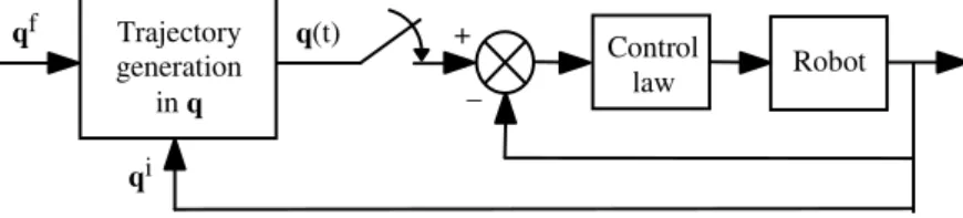
8.2. Trajectory generation and control loops ... 188 

8.3. Point-to-point trajectory in the joint space ... 189 

8.3.1. Polynomial interpolation ... 190 

8.3.1.1. Linear interpolation ... 190 

8.3.1.2. Cubic polynomial ... 190 

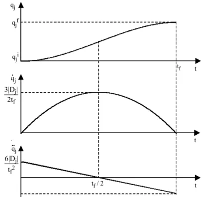
8.3.1.3. Quintic polynomial ... 191 

8.3.1.4. Computation of the minimum traveling time ... 193 

8.3.2. Bang-bang acceleration profile ... 194 

8.3.3. Trapezoidal velocity model ... 195 

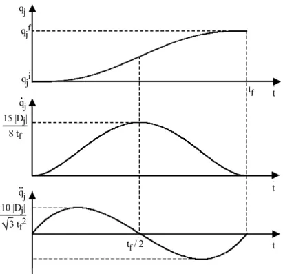
8.3.4. Continuous acceleration profile with constant velocity phase ... 201 

8.4. Point-to-point trajectory in the task space ... 204 

Motion control ... 209 

9.1. Introduction ... 209 

9.2. Equations of motion ... 209 

9.3. PID control ... 210 

9.3.1. PID control in the joint space ... 210 

9.3.2. Stability analysis ... 212 

9.3.3. PID control in the task space ... 214 

9.4. Linearizing and decoupling control ... 215 

9.4.1. Introduction ... 215 

9.4.2. Computed torque control in the joint space ... 216 

9.4.2.1. Principle of the control ... 216 

9.4.2.2. Tracking control scheme ... 217 

9.4.2.3. Position control scheme ... 218 

9.4.2.4. Predictive dynamic control ... 219 

9.4.2.5. Practical computation of the computed torque control laws ... 219 

9.4.3. Computed torque control in the task space ... 220 

9.7. Conclusion ... 222  Appendix: Dynamic model of Staubli 90

Chapter 7

Dynamic modeling of serial robots

7.1. Introduction

The inverse dynamic model provides the joint torques and forces in terms of the joint positions, velocities and accelerations. It is described by:

= f(q, .q, ..q, F_e) [7.1]

with:

• : vector of joint torques or forces, depending on whether the joint is revolute or prismatic respectively. In the sequel, we will only write joint torques; • q: vector of joint positions;

• q: vector of joint velocities; . • ..q: vector of joint accelerations;

• F_e: vector of forces and moments exerted by the robot on the environment. Equation [7.1] is an inverse dynamic model because it defines the system input as a function of the output variables. It is often called the dynamic model. This form of model which is expressed in terms of Lagrangian variables (joint variables and their derivatives) is called “Lagrangian Model”. The Euler model makes use of the Eulerian variables (linear and rotational Cartesian velocities and accelerations).

The direct dynamic model gives the joint accelerations in terms of the joint positions, velocities and torques. It is represented by the relation:

..

The dynamic model of robots plays an important role in their design and control. For robot design, the inverse dynamic model can be used to select the actuators [Chedmail 90b], [Potkonjak 86], while the direct dynamic model is employed to carry out simulations (§ 7.7) for the purpose of testing the performance of the robot and to study the relative merits of possible control schemes. Regarding robot control, the inverse dynamic model is used to compute the actuator torques, which are needed to achieve a desired motion . It is also used to identify the dynamic parameters that are necessary for both control and simulation applications .

Several approaches have been proposed to model the dynamics of robots [Renaud 75], [Coiffet 81], [Vukobratovic 82]. The most frequently employed in robotics are the Lagrange formulation [Uicker 69], [Khalil 76], [Renaud 80a], [Hollerbach 80], [Paul 81], [Megahed 84], [Renaud 85] and the Newton-Euler formulation [Hooker 65], [Armstrong 79], [Luh 80b], [Orin 79], [Khalil 85a], [Khosla 86], [Khalil 87b], [Renaud 87].

In this chapter, we present the dynamic modeling of serial robots using these two formulations. The problem of calculating a minimum set of inertial parameters (base parameters) will not be covered in this year. We will focus our study on the minimization of the number of operations of the dynamic model in view of its real time computation for control purposes. Lastly, the computation of the direct dynamic model will be addressed.

7.2. Notations

The main notations used in this chapter are compiled below: aj unit vector along axis zj;

F_tj total external wrench (forces and moments) on link j, composed of f_tj and m_tj;

f_j force exerted on link j by link j – 1; f_ej force exerted by link j on the environment; F_cj parameter of Coulomb friction acting at joint j; F_vj parameter of viscous friction acting at joint j; g gravitational acceleration;

G_j center-of-mass of link j;

I_Gj inertia tensor of link j about G_j and with respect to a frame parallel to frame R_j;

Ia_j moment of inertia of the rotor and the transmission system of actuator j referred to the joint side;

2 2 j j j j 2 2 Oj j j j 2 2 j j j (y z ) dm xy dm xzdm XX XY XZ = xy dm (x z ) dm yz dm XY YY YZ XZ YZ ZZ xz dm yz dm (x y )dm  _{  }  _{ }  _{  }         _{  }         



















I [7.3]

Ij (6x6) spatial inertia matrix of link j (relation [7.21]);

L_j position vector between O_j-1 and O_j; M_j mass of link j;

MS_j first moments of link j with respect to frame R_j, equal to M_j S_j. The components of j_{MSj are denoted by [ MXj MYj MZj ]}T_;

m_Gj moment of external forces on link j about G_j; mtj moment of external forces on link j about Oj;

mj moment about Oj exerted on link j by link j – 1;

mej moment about Oj exerted by link j on the environment;

s_j vector of the center-of-mass coordinates of link j. It is equal to O_jG_j; v_j linear velocity of O_j;

Vj (6x1) kinematic screw vector of link j, formed by the components of vj and _j;

j

v

linear acceleration of O_j;

v_Gj linear velocity of the center-of-mass of link j;

Gj

v

linear acceleration of the center-of-mass of link j; _j angular velocity of link j;

._j angular acceleration of link j.

7.3. Lagrange formulation 7.3.1. Introduction

The dynamic model of a robot with several degrees of freedom represents a complicated system. The Newton-Euler method developed in § 7.5 presents an efficient and systematic approach to solving this problem. In this section, we develop a simple Lagrange method to present the general form of the dynamic model of robots and to get an insight into its properties. Firstly, we consider an ideal system without friction or elasticity, exerting neither forces nor moments on the environment. These phenomena will be covered in § 7.3.4 through 7.3.8.

The Lagrange formulation describes the behavior of a dynamic system in terms of work and energy stored in the system. The Lagrange equations are written in the form:

i i i d L L = for i = 1, ..., n dt q q       [7.4a]

This relation can be written in matrix form as:

d

dt













 

_

_



_

_







q







q



T T

L

L

where L is the Lagrangian of the robot defined as the difference between the kinetic energy E and the potential energy U of the system:

L = E – U [7.4b]

7.3.2. General form of the dynamic equations

The kinetic energy of the system is a quadratic function in the joint velocities such that:

E = 1_{2 q}.T _Aq.

[7.5]

where A is the (nxn) symmetric and positive definite inertia matrix of the robot. Its elements are functions of the joint positions. The (i, j) element of A is denoted by A_ij.

Since the potential energy is a function of the joint positions, equations [7.4] and [7.5] lead to:

= ( ) + ( , ) + ( ) A q q C q q q Q q

 [7.6]

where:

• C(q, q.) q. is the (nx1) vector of Coriolis and centrifugal torques, such that: C q. = A. q. – ∂E_∂q

• Q = [Q₁ … Q_n]T _{is the vector of gravity torques.}

Consequently, the dynamic model of a robot is described by n coupled and nonlinear second order differential equations.

There exist several forms for the vector C(q, q.) q.. Using the Christoffell symbols c_i,jk, the (i, j) element of the matrix C can be written as:

n ij i, jk k k 1 ij _ik jk i, jk k j i C c q A _A A 1 c [ ] 2 q q q       _{ }   _{  }  _{  } 



 [7.7]

The Q_i element of the vector Q is calculated according to: i i U Q q    [7.8]

The elements of A, C and Q are functions of the geometric and inertial parameters of the robot.

7.3.3. Computation of the elements of A, C and Q

To compute the elements of A, C and Q, we begin by symbolically computing the expressions of the kinetic and potential energies of all the links of the robot. Then, we proceed as follows:

i – the element A_ij is equal to i j

E q q 

  this leads to:

- the element A_ii is equal to the coefficient of (q._i2_{/2) in the expression of the} kinetic energy, while A_ij, for i ≠ j, is equal to the coefficient of q._i q._j;

ii –the elements of C are obtained from equation [7.7]; iii–the elements of Q are obtained from equation [7.8]. 7.3.3.1. Computation of the kinetic energy

The kinetic energy of the robot is given as: n j j 1 E E  



[7.9]

T T j j Gj j j Gj Gj 1 E ( M ) 2   I   v v [7.10]

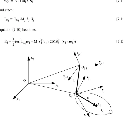
Since the velocity of the center-of-mass can be expressed as (Figure 7.1):

VGj = Vj + j x Sj [7.11] and since: Oj Gj j j j= -M I I s s  [7.12] equation [7.10] becomes: Oj T T T j 1 j j j j j j j j E ( M 2 ( )) 2    ω I ω  v v MS v ω [7.13] O_j x_j-1 x_j s_j z_j-1 O₀ x₀ y₀ z₀ y_j-1 z_j L_j O_j-1 G_j C_j y_j

Figure 7.1. Composition of velocities

Equation [7.10] is not linear in the coordinates of the vector S_j. On the contrary, equation [7.13] is linear in the elements of M_j, MS_j and J_j, which we call the

standard inertial parameters. The linear and angular velocities V_j and _j are computed using the following recursive equations (Figure 7.1):

_j_j-1 +–_jq._j a_j [7.14]

If the base of the robot is fixed, the previous equations are initialized by v₀ = 0 and₀ = 0.

All the elements appearing in equation [7.13] must be expressed in the same frame. The most efficient way is to express them relative to frame R_j which is fixed with the link j. Therefore, equations [7.13], [7.14] and [7.15] are rewritten as:

E_j = 1_{2 [}j_ jT jIOj jj + MjjvjTjvj + 2 jMSjT (jvj x jj)] [7.16] j_ j  jRj-1j-1j-1 +–jq.jjaj  jj-1 +–jq.jjaj [7.17] j_{vj =} j_{Rj-1 (}j-1_{vj-1 +} j-1_{j-1 x} j-1_{Pj) + j q}._jj_{aj [7.18]} The parameters j_I

Oj and jMSj are constants.

Using the spatial notation, the kinetic energy can be written in the following compact form by using screw notations:

Ej = 1₂ jVTj jIj jVj [7.19] where: j_{Vj =}













j_vj j_j [7.20] j_{Ij =} j T j j j j j Oj ˆ M ˆ         3 I MS MS I [7.21] where jMSˆT_j =  MSj ˆ_j

The recursive velocity relations [7.17] and [7.18] can be combined as follows: j_{Vj =} j_Sj-1 j-1_{Vj-1 + q}._j j_{aj [7.22]} where j_{Sj-1 is the (6x6) screw transformation matrix defined in [2.46] as:}

j_S j-1 =













j_R j-1 –jRj-1j-1P^j 0₃ j_R j-1 =













j_R j-1 jP^j-1jRj-1 0₃ j_R j-1 [7.23a]

j_{aj =}













_j j_aj – _j j_a j [7.23b]

7.3.3.2. Computation of the potential energy The potential energy is given by:

n n T j j 0, j j j 1 j 1 U U M ( )   



 



g L s [7.24]

where L_{0, j} is the position vector from the origin O₀ to O_j. Projecting the vectors appearing in [7.24] into frame R₀, we obtain:

0 T 0 0 j

j j j j j

U  M g ( P  R S ) [7.25a]

an expression that can be rewritten linearly in M_j and the elements of j_{MSj as:}

j 0 T 0 0 j 0 T 0 j j j j j j j j U (M ) 0 M     _{ }    _{   }     MS g P R MS g T [7.25b]

Since the kinetic and potential energies are linear in the elements of j_I

Oj, jMSj, M_j, we deduce that the dynamic model is also linear in these parameters.

7.3.3.3. Dynamic model properties

In this section, we summarize some important properties of the dynamic model of robots:

a) the inertia matrix A is symmetric and positive definite; b) the energy of link j is a function of (q1, …, qj) and (q.1, …, q.j);

c) the element Aij is a function of qk+1, …, qn,with k = min(i, j), and of the inertial parameters of links r, ..., n, with r = max(i, j);

d) from property b and equation [7.4], we deduce that _i is a function of the inertial parameters of links i, ..., n;

e) the matrix [d -2 ( , )]

dtA C q q is skew-symmetric for the choice of the matrix C given by equation [7.7] [Koditschek 84], [Arimoto 84]. This property is used in Chapter 14 for the stability analysis of certain control schemes;

f) the inverse dynamic model is linear in the elements of the standard inertial parameters M_j, j_MS

j and jJj. This property is exploited to identify the dynamic parameters (inertial and friction parameters), to reduce the computation burden of the dynamic model, and to develop adaptive control schemes; g) there exist some positive real numbers a1, ..., a7 such that for any values of q

and q. we have [Samson 87]: || A(q) || ≤ a₁ + a₂ || q || + a₃ || q ||2 || C(q, q.) || ≤ || q. || (a4 + a5 || q ||) || Q || ≤ a6 + a7 || q ||

where ||*|| indicates a matrix or vector norm. If the robot has only revolute joints, these relations become:

|| A(q) || ≤ a₁ || C(q, q.) || ≤ a₄ || q. || || Q || ≤ a₆

h) a robot is a passive system which dissipates energy. This property is related to property e).

7.3.4. Considering friction

Friction plays a dominant role in limiting the quality of robot performance. Non-compensated friction produces static error, delay, and limit cycle behavior [Canudas de Wit 90]. Many works have been devoted to studying friction torque in the joint and transmission systems. Various friction models have been proposed in the literature [Dahl 77], [Canudas de Wit 89], [Armstrong 88], [Armstrong 91], [Armstrong 94]. In general, three kinds of frictions are noted: Coulomb friction, static friction, and viscous friction.

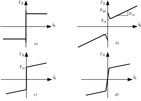
The model based on Coulomb friction assumes a constant friction component that is independent of the magnitude of the velocity. The static friction is the torque necessary to initiate motion from rest. It is often greater than the Coulomb friction (Figure 7.2a). The viscous friction is generally represented as being proportional to the velocity, but experimental studies [Armstrong 88] have pointed out the Stribeck phenomenon that arises from the use of fluid lubrication. It results in decreasing friction with increasing velocity at low velocity, then the friction becomes

proportional to velocity (Figure 7.2b). A general friction model describing these components is given by:

_fi = F_ci sign(q.i) + Fviq.i + (Fsti – Fci) sign(q.i) e–|q.i|Bi [7.26] In this expression, _fi denotes the friction torque of joint i, F_ci and F_vi indicate

the Coulomb and viscous friction parameters respectively. The static torque is equal to F_sti sign(q._i). . q_i Fsti Fvi fi a) b) Fci d) c) _fi fi _fi . qi q.i . q_i Fci

Figure 7.2. Friction models

The most often employed model is composed of Coulomb friction together with viscous friction (Figure 7.2c). Therefore, the friction torque at joint i is written as:

_fi = F_ci sign(q._i) + F_viq._i [7.27]

To take into account the friction in the dynamic model of a robot, we add the vector _f on the right side of equation [7.6] such that:

_f = diag(q.)F_v + diag(sign(q.))F_c [7.28]

• F_v =

[

Fv1 ... Fvn T

]

; • Fc =

[

Fc1 ... Fcn T

]

;

• diag(q) is the diagonal matrix whose elements are the components of . q. . This friction model can be approximated by a piecewise linear model as shown in Figure 7.2d.

7.3.5. Considering the rotor inertia of actuators

The kinetic energy of the rotor (and transmission system) of actuator j, is given by the expression1 Ia q_{j j}2

2  . The inertial parameter Iaj denotes the equivalent inertia referred to the joint velocity. It is given by:

2

j j

Ia = Nj Jm [7.29]

where Jmj is the moment of inertia of the rotor and transmissions of actuator j, Nj is the transmission ratio of joint j axis, equal to q.mj / q.j where q.mj denotes the rotor velocity of actuator j. In the case of a prismatic joint, Iaj is an equivalent mass.

In order to consider the rotor inertia in the dynamic model of the robot, we add the inertia (or mass) Ia_j to the A_jj element of the matrix A, that is to say we add the term Ia q_{j j}on j.

Note that such modeling neglects the gyroscopic effects of the rotors, which take place when the actuator is fixed on a moving link. However, this approximation is justified for high gear transmission ratios. For more accurate modeling of the rotors the reader is referred to [Llibre 83], [Chedmail 86], [Murphy 93], [Sciavicco 94]. 7.3.6. Considering the forces and moments exerted by the end-effector on the

environment

We have seen in § 5.9 that the joint torque vector _e necessary to exert a given wrench fen on the environment is obtained using the basic static equation:

_e = JT_nFen [7.30]

7.3.7. Relation between joint torques and actuator torques

In general, the joint variables are not equal to the motor variables because of the existence of transmission systems or because of couplings between the actuator variables. The relation between joint torques and actuator torques can be obtained using the principle of virtual work. Let the relationship between the infinitesimal joint displacement dq and the infinitesimal actuator variable dq_m be given by:

dq =J_qm dq_m [7.31]

where J_qmis the Jacobian of q with respect to q_m, equal to _∂∂_qq m . The virtual work can be written as:

T _dq* _=T_mdq*_{m [7.32]}

where _mis the actuator torque vector and the superscript (*_{) indicates virtual} displacements.

Combining equations [7.31] and [7.32] yields:

_m= JT_qm  [7.33]

7.3.8. Modeling of robots with elastic joints

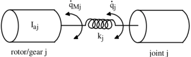
The presence of joint flexibility is a common feature of many current industrial robots. The joint elasticity may arise from several sources, such as elasticity in the gears, transmission belts, harmonic drives, etc. It follows that a time-varying displacement is introduced between the position of the driving actuator and the joint position. The joint elasticity is modeled as a linear torsional spring for revolute joints and a linear spring for prismatic joints [Khalil 78], [Spong 87]. Thus, the dynamic model requires twice the number of generalized coordinates to completely characterize the configuration of the links and the rotors of the actuators. Let q_M denotes the (nx1) vector of rotor positions as reflected through the gear ratios (Figure 7.3). Consequently, the vector of joint deformations is given by (q – q_M). Note that the direct geometric model is only a function of the joint variables q.

The potential energy of the springs is given by: U_k = 1_{2 (q – qM})T _{k (q – q}

where k is the (nxn) definite positive joint stiffness matrix.

The dynamic equations are obtained using the Lagrange equation, i.e.: A ..q+ C q + Q + k (q. _{– q}

M) + diag(q) F. v + diag(sign(q)) F. c = 0 [7.35a]

Ia ..qM +diag(q.M) Fvm + diag(sign(q.M)) Fcm – k(q – qM) =  [7.35b] where I_a is the (nxn) diagonal matrix containing the inertia of the rotors, F_vm and F_cm are the (nx1) vectors containing the viscous and Coulomb parameters of the actuators and transmissions referred to the joint side. The joint friction terms can easily be included in equation [7.35a].

A general and systematic method to model systems with lumped elasticity is presented in [Khalil 00a].

kj joint j rotor/gear j Iaj . q_Mj q._j

Figure 7.3. Modeling of joint flexibility

•

Example 7.1. Computation of the elements of the matrices A and Q for the first three links of the Stäubli RX-90 robot whose geometric parameters are given in Example 3.1.

i) computation of the angular velocities (equation [7.17])

0_{0 = 0} 1_{1 = [ 0 0 q}._1]T 2_ 2 = 2R111 +q.2 2a2 =

















C2 0 S2 –S2 0 C2 0 –1 0













0 0 . q₁ +













0 0 . q₂ = [S2 q.₁ C2 q.₁ q.₂]T 3_ 3 = 3R222 + q.3 3a3

=

















C3 S3 0 –S3 C3 0 0 0 1

















S2q.₁ C2 q.₁ . q₂ +













0 0 . q3 = [S23 q.₁ C23 q.₁ q._{2 +} q.₃]T

ii) computation of the linear velocities (equation [7.18])

0_{v0 = 0} 1_{v1 = 0} 1_v 2 = 1v1 + 11 x 1P2 = 0 2_{v2 = 0} 2_v 3 = 22 x 2P3 = [0 D3 q.2 –C2D3 q.1]T 3_{v3 =} 3_R22_{v3 = [S3 D3 q}._{2 C3 D3 q}._{2 –C2D3 q}._1]T

iii) computation of the inertia matrix A. With the following general inertial

parameters: j_{MSj = [MXj MYj MZj]T} j j j j Oj j j j j j j XX XY XZ = XY YY YZ XZ YZ ZZ             I , a1 a a2 a3 I 0 0 = 0 I 0 0 0 I           I

we obtain the elements of the robot inertia matrix as:

A11 = Ia1 + ZZ1 + SS2 XX2 + 2CS2 XY2 + CC2 YY2 + SS23 XX3 + 2CS23 XY₃ + CC23 YY₃ + 2C2 C23 D3 MX₃ – 2C2 S23 D3 MY₃ + CC2 D32 M₃ A₁₂ = S2 XZ₂ + C2 YZ₂ + S23 XZ₃ + C23 YZ₃ – S2 D3 MZ₃ A13 = S23 XZ3 + C23 YZ3 A₂₂ = Ia₂ + ZZ₂ + ZZ₃ + 2C3 D3 MX₃ – 2S3 D3 MY₃ + D32 _M 3 A₂₃ = ZZ₃ + C3 D3 MX₃ – S3 D3 MY₃ A₃₃ = Ia₃ + ZZ₃

where SSj = (sin _j)2_{,CCj = (cos j)}2 _{andCSj = cos j sin j. The elements of the} matrix C can be computed by equation [7.7];

iv) computation of the gravity forces. Assuming that gravitational acceleration is

given as 0_{g = [0 0 G3]}T_{, and using equation [7.25], the potential energy is} obtained as:

U = –G3 (MZ₁ + S2MX₂ + C2MY₂ + S23MX₃ + C23MY₃ + D3S2M₃) Using equation [7.8] gives:

Q₁ = 0

Q₂ = –G3 (C2 MX₂ – S2 MY₂ + C23 MX₃ – S23 MY₃ + D3 C2 M₃) Q₃ = –G3 (C23 MX₃ – S23 MY₃)

7.4. Newton-Euler formulation 7.4.1. Introduction

The Newton-Euler equations describing the forces and moments (wrench) acting on the center-of-mass of link j are given as:

j j Gj Gj Gj j j Gj j = M [7.36] = + ( ) [7.37] f v m I ω ω I ω  

The Newton-Euler algorithm of Luh, Walker and Paul [Luh 80b], which is considered as one of the most efficient algorithms for real time computation of the inverse dynamic model, consists of two recursive computations: forward recursion and backward recursion. The forward recursion, from the base to the terminal link, computes the link velocities and accelerations and consequently the dynamic wrench on each link. The backward recursion, from the terminal link to the base, provides the reaction wrenches on the links and consequently the joint torques.

This method gives the joint torques as defined by equation [7.1] without explicitly computing the matrices A, C and Q. The model obtained is not linear in the inertial parameters because it makes use of Mj, Sj andIGj.

7.4.2. Newton-Euler inverse dynamics linear in the inertial parameters

In this section, we develop a Newton-Euler algorithm based on the double recursive computations of Luh et al. [Luh 80b], but which uses as inertial parameters the elements of Jj, MSj and Mj [Khalil 87b], [Khosla 86]. The dynamic wrench on link j is calculated on Oj and not on the center of gravity Gj. Therefore, the resulting model is linear in the dynamic parameters. This reformulation allows

us to compute the dynamic model in terms of the base inertial parameters (minimum inertial parameters) and to use it for the identification of the dynamic parameters.

The Newton-Euler equations giving the forces and moments of link j at the origin of frame R_j are given as:

tj j j j j j j j tj Oj j j j j Oj j = M + ( ) [7.38] = + + ( ) [7.39]       f v ω MS ω ω MS m I ω MS v ω I ω    

Using the spatial notation, we can write these equations as: tj F = Ij j j j j Oj j ( ) j _{( )}             ω ω MS ω I ω V [7.40] where j j tj tj j tj ,                v ω f F V m  

 _{Ij is the spatial inertia matrix (equation [7.21]).}

i) forward recursive computation: to compute f_tj and m_tj for j = 1, …, n, using equations [7.38] and [7.39], we need _j, ._j and v._j..The velocities are given by the recursive equations [7.14] and [7.15] rewritten hereafter as:



_j = _j-1 + –_jq._j a_j [7.41]

vj = vj-1 + j-1 x Lj + jq.j aj [7.42]

Differentiating equations [7.41] and [7.42] with respect to time gives:

._j = ._j-1 + –_j (..q_j a_j + _j-1 x q._j a_j) [7.43] and v._j = v._j-1 + ._j-1 x L_j + _j-1 x (_j-1 x L_j+ _jq._j a_j) + _j (..q_j a_j + _j-1 x q._j a_j) giving V.j = V.j-1 + .j-1 x Lj + j-1 x (j-1 x Lj) + j (..qj aj + 2 j-1 x q.j aj) [7.44] 

The initial conditions for a robot with a fixed base are ₀= 0, .₀ = 0 and and v.₀ = 0.

ii) backward recursive computation: this is based on writing for each link j, for j =

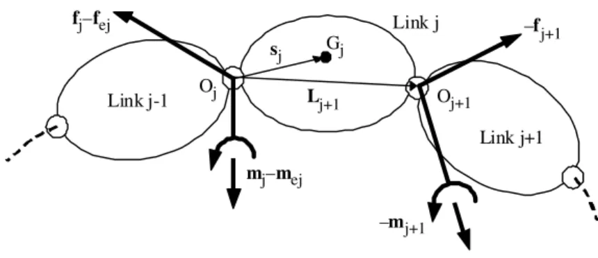
n,…,1, the Newton-Euler equations at the origin O_j, as follows (Figure 7.5):

f_tj = f_j – f_j+1 + M_j g – f_ej [7.45]

G_j –m_j+1 s_j L_j+1 –f_j+1 O_{j O} j+1 f_j–f_ej m_j–m_ej Link j-1 Link j+1 Link j

Figure 7.5. Forces and moments on link j

We note that f_ej and m_ej, which represent the force and moment exerted by link j on the environment,may include contributions from springs, dampers, contact with the environment, etc. Their values are assumed to be known, or at least to be calculated from known quantities.

We can cancel the gravity terms from equations [7.45] and [7.46] and take into account their effects by setting up the initial linear acceleration such that:

v.₀ = –g [7.47]

Thus, using equations [7.45] and [7.46], we obtain:

f_j = f_tj + f_j+1 + f_ej [7.48]

m_j = m_tj + m_j+1+ L_j+1 x f_j+1 + m_ej [7.49]

This backward recursive algorithm is initialized by fn+1 = 0 and mn+1 = 0. Finally, the joint torque j can be obtained by projecting fj or mj on the joint axis, depending whether the joint is prismatic or revolute respectively. We can also consider the friction forces and the rotor inertia as shown in the Lagrange method:

_j = (j fj + –j mj)T aj + Fcj sign(q.j) + Fvjq.j + Iaj..qj [7.50] From equations [7.48], [7.49] and [7.50], we deduce that _j is a function of the inertial parameters of links j, j + 1, …, n. This property has been outlined in § 7.3.3.3.

Since I_Oj and MS_j are constants when referred to their own link coordinates, the Newton-Euler algorithm can be efficiently computed by referring the velocities, accelerations, forces and moments to the local link coordinate system [Luh 80b]. The forward recursive equations become, for j = 1, ..., n:

j_{j-1 =} j_Rj-1j-1_{j-1 [7.51]} j_{j =} j_{j-1 + –jq}._jj_{aj [7.52]} j_. j = jRj-1j-1.j-1 + –j (..qj jaj + jj-1 x q.j jaj) [7.53] j_v._{j =} j_{Rj-1 (}j-1_v._{j-1 +} j-1_Uj-1j-1_{Pj) + j (}.._qj j_{aj + 2} j_{j-1 x q}._jj_{aj) [7.54]} j_{ftj = Mj} j_v._{j +} j_Ujj_{MSj [7.55]} j_m tj = jIOj j.j + jMSj x jv . j + jj x (jIOjjj) [7.56] j_U j = j.^j + j^jj^j [7.57] For a stationary base, the initial conditions are ₀ = 0, .₀ = 0 and v.₀ = – g. The use of j_U

j saves 21n multiplications and 6n additions in the computation of the inverse dynamic model of a general robot [Kleinfinger 86a].

The backward recursive equations, for j = n, ..., 1, are:

j_{fj =} j_{ftj +} j_{fj+1 +} j_{fej [7.58]} j-1_f j = j-1Rjjfj [7.59] j_m j = jmtj + jRj+1j+1mj+1 + jPj+1 x jfj+1 + jmej [7.60] _j = (_jj_f j + –jjmj)Tjaj + Fsj sign(q.j) + Fvjq.j + Iaj..qj [7.61] The previous algorithm can be numerically programmed for a general serial

robot. Its computational complexity is O(n), which means that the number of operations is linear in the number of degrees of freedom. However, as we will see in the next section, the use of the base inertial parameters in a customized symbolic algorithm considerably reduces the number of operations of the dynamic model. NOTES:-

- the symbol jv_j means jR v₀0 _j , and not the time derivative of jv_j. Using the fact that:

0 j j

j 0 j

v R v and0R_j 0ω Rˆ_j0 _j

j j j j j j j j 0 0 0 0 0 j 0 0 j j j j j j j j j 0 j j 0 j 0 j j 0 j 0 j j j j d dt since d _{ˆ ˆ ˆ} dt            v v ω v v R ω v R v R ω R R v R v ω v v      . On the contrary, j _j d j _j j ₀0 _j dt   ω ω R ω .

- We use j =2 to define a fixed frame Rj with resoect to j-1. In this case q._j and ..q_j

are equal to zero, the torque equation [9.94] has no physical meaning and should not be calculated, whereas the velocity and acceleration equations can be used after eliminating the terms multiplied by j or –j .

- If link 0, the base, is mobile (not fixed) with r dof (car, walking robot, or mobile manipulator), we can represent its motion using r virtual joints (Lagrangian variables). The inertial parameters of the first r-1 virtual links are taken equal to zero whereas the rth _{link parameters are equal to those of the base. This case is} efficient if the motion is in a plane. The mobile motion can be represented by two prismatic joints followed by a rotational joint.

- If link 0, the base is mobile, it is in general more efficient to represent its motion using Eulerian variables (linear and rotational Cartesian velocities and accelerations). The equations of the base will be represented in Eulerian form.

7.5. Real time computation of the inverse dynamic model 7.5.1. Introduction

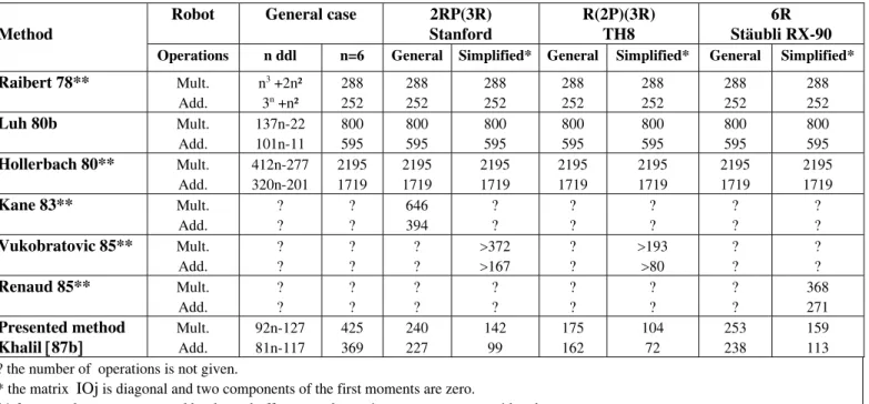
Much work has been focused on the problem of computational efficiency of the inverse dynamic model of robots in order to realize real time dynamic control. This objective is now recognized as being attained (Table 7.5).

Before describing our method, which is based on a customized symbolic Newton-Euler formulation linear in the inertial parameters [Khalil 87b], [Kleinfinger 86a], we review the main approaches presented in the literature.

The Lagrangian formulation of Uicker and Kahn [Uicker 69], [Kahn 69] served as a standard robot dynamics formulation for over a decade. In this form, the complexity of the equations precluded the real time computation of the inverse dynamic model. For example, for a six degree-of-freedom robot, this formulation requires 66271 multiplications and 51548 additions [Hollerbach 80]. This led researchers to investigate either simplification or tabulation approaches to achieve real time implementation.

The first approach towards simplification is to neglect the Coriolis and centrifugal terms with the assumption that they are not significant except at high speeds [Paul 72], [Bejczy 74]. Unfortunately, this belief is not valid: firstly, Luh et al. [Luh 80b] have shown that such simplifications leads to large errors not only in the value of the computed joint torques but also in its sign; later, Hollerbach [Hollerbach 84a] has shown that the velocity terms have the same significance relative to the acceleration terms whatever the velocity.

An alternative simplification approach has been proposed by Bejczy [Bejczy 79]. This approach is based on an exhaustive term-by-term analysis of the elements A_ij, C_i,jk and Q_i so that the most significant terms are only retained. A similar procedure has been utilized by Armstrong et al. [Armstrong 86] who also proposed computing the elements A_ij, C_i,jk and Q_i with a low frequency rate with respect to that of the servo rate. Using such an analysis for a six degree-of-freedom robot becomes very laborious and tedious.

In the tabulation approach, some terms of the dynamic equations are precomputed and tabulated. The combination of a look-up table with reduced analytical computations renders them feasible in real time. Two methods based on a trade-off between memory space and computation time have been investigated by Raibert [Raibert 77]. In the first method SSM (State Space Model), the table was carried out as a function of the joint positions and velocities (q and q.), but the required memory was too big to consider in real applications at that time. In the

Configuration Space Method (CSM), the table is computed as a function of the joint

positions. Another technique, proposed by Aldon [Aldon 82] consists of tabulating the elements A_ij and Q_i and of calculating the elements C_i,jk on-line in terms of the A_ij elements. This method considerably reduces the required memory but increases the number of on-line operations, which becomes proportional to n3_{. We note that} the tabulated elements are functions of the load inertial parameters, which means making a table for each load.

Luh et al. [Luh 80a] proposed to determine the inverse dynamic model using a Newton-Euler formulation (§ 7.5). The complexity of this method is O(n). This method has proved the importance of the recursive computations and the organization of the different steps of the dynamic algorithm. Therefore, other researchers tried to improve the existing Lagrange formulations by introducing recursive computations. For example, Hollerbach [Hollerbach 80] proposed a new recursive Lagrange formulation with complexity O(n), whereas Megahed [Megahed 84] developed a new recursive computational procedure for the Lagrange method of Uicker and Kahn. However, these methods are less efficient than the Newton-Euler formulation of Luh et al. [Luh 80a].

More recently, researchers investigated alternative formulations [Kane 83], [Vukobratovic 85], [Renaud 85], [Kazerounian 86], but the recursive Newton-Euler proved to be computationally more efficient.

The most efficient models proposed until now are based on a customized symbolic Newton-Euler formulation that takes into account the particularity of the

geometric and inertial parameters of each robot [Kanade 84], [Khalil 85a], [Khalil 87b], [Renaud 87]. Moreover, the use of the base inertial parameters in this algorithm reduces the computational cost by about 25%. We note that the number of operations for this method is even less than that of the tabulated CSM method.

Table 7.5. Computational cost of the inverse dynamic modeling methods Method

Robot General case 2RP(3R)

Stanford

R(2P)(3R) TH8

6R Stäubli RX-90

Operations n ddl n=6 General Simplified* General Simplified* General Simplified*

Raibert 78** Mult. Add. n3 _+2n² 3n _+n² 288 252 288 252 288 252 288 252 288 252 288 252 288 252 Luh 80b Mult. Add. 137n-22 101n-11 800 595 800 595 800 595 800 595 800 595 800 595 800 595 Hollerbach 80** Mult. Add. 412n-277 320n-201 2195 1719 2195 1719 2195 1719 2195 1719 2195 1719 2195 1719 2195 1719 Kane 83** Mult. Add. ? ? ? ? 646 394 ? ? ? ? ? ? ? ? ? ? Vukobratovic 85** Mult. Add. ? ? ? ? ? ? 372 167 ? ? 193 80 ? ? ? ? Renaud 85** Mult. Add. ? ? ? ? ? ? ? ? ? ? ? ? ? ? 368 271 Presented method Khalil 87b Mult. Add. 92n-127 81n-117 425 369 240 227 142 99 175 162 104 72 253 238 159 113 ? the number of operations is not given.

* the matrix IOj is diagonal and two components of the first moments are zero.

** forces and moments exerted by the end-effector on the environment are not considered.  the given number of operations corresponds to the computation of the elements of A, Ci,jk and Q.

Before closing this section, it is worth noting the formidable technological progress in the field of computer processors, to the point that the dynamic model can be calculated at control rate with standard personal computers (Chapter 14). 7.5.2. Customization of the Newton-Euler formulation

The recursive Newton-Euler formulation of robot dynamics has become a standard algorithm for real time control and simulation (§ 7.5.3). To increase the efficiency of the Newton-Euler algorithm, we generate a customized symbolic model for each specific robot and utilize the base dynamic parameters. To obtain this model, we expand the recursive equations to transform them into scalar equations without incorporating loop computations. The elements of a vector or a matrix containing at least one mathematical operation are replaced by an intermediate variable. This variable is written in the output file, which contains the customized model [Kanade 84], [Khalil 85a]. The elements that do not contain any operation are not modified. We propagate the obtained vectors and matrices in the subsequent equations. Consequently, customizing eliminates multiplications by one (and minus one) and zero, and additions with zero. A good choice of the intermediate variables allows us to avoid redundant computations. In the end, the dynamic model is obtained as a set of intermediate variables. Those that have no effect on the desired output, the joint torques in the case of inverse dynamics, can be eliminated by scanning the intermediate variables from the end to the beginning.

The customization technique allows us to reduce the computational load for a general robot, but this reduction is larger when carried out for a specific robot [Kleinfinger 86a]. The computational efficiency in customization is obtained at the cost of a software symbolic iterative structure [Khalil 97] and a relatively increased program memory requirement.

•

Example 7.4. To illustrate how to generate a customized symbolic model, we develop in this example the computation of the link angular velocities j_{j for the} Stäubli RX-90 robot. The computation of the orientation matricesj-1_{Aj (Example} 3.3) generates the 12 sinus and cosinus intermediate variables:

Sj = sin(q_j)

Cj = cos(qj) for j = 1, …, 6

The computation of the angular velocities for j = 1, …, 6 is given as: 1_ 1 =













0 0 QP1

Computation of 1_{1 does not generate any intermediate variable.} 2_ 1 =













S2*QP1 C2*QP1 0 =













WI12 WI22 0 Computation of 2_

2 generates the following intermediate variables: WI12 = S2*QP1

WI22 = C2*QP1

In the following, the vector 2_{2 is set as:} 2_{2 =}













WI12 WI22 QP2

Continuing the recursive computation leads to: 3_{2 =}













C3*WI12 + S3*WI22 –S3*WI12 + C3*WI22 QP2 =













WI13 WI23 QP2 3_{3 =}













WI13 WI23 QP2 + QP3 =













WI13 WI23 W33 4_ 3 =













C4*WI13 – S4*W33 –S4*WI12 – C4*W33 WI23 =













WI14 WI24 WI23 4_ 4 =













WI14 WI24 WI23 + QP4 =













WI14 WI24 W34 5_{4 =}













C5*WI14 + S5*W34 –S5*WI14 + C5*W34 –WI24 =













WI15 WI25 –WI24 5_{5 =}













WI15 WI25 –WI24 + QP5 =













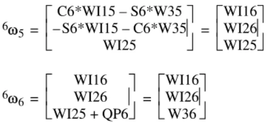
WI15 WI25 W35

6_{5 =}













C6*WI15 – S6*W35 –S6*WI15 – C6*W35 WI25 =













WI16 WI26 WI25 6_ 6 =













WI16 WI26 WI25 + QP6 =













WI16 WI26 W36 Finally, the computation of j_

j, for j = 1, …, 6, requires the following intermediate variables: WI12, WI22, WI13, WI23, W33, WI14, WI24, W34, WI15, WI25, W35, WI16, WI26 and W36, in addition to the variables Sj and Cj for j = 2, …, 6. The variables S1 and C1 can be eliminated because they have no effect on the angular velocities.

7.5.3. Utilization of the base inertial parameters

The dynamic model can be obtained in a reduced number of inertial parameters called the base inertial parameters. These parameters are obtained from the standard parameters after eliminating those who have no effect on the dynamic model and by grouping some parameters together. It is obvious that the use of the base inertial parameters in a customized Newton-Euler formulation that is linear in the inertial parameters will reduce the number of operations because the parameters that have no effect on the model or have been grouped are set equal to zero. Practically, the number of operations of the inverse dynamic model when using the base inertial parameters for a general n revolute degree-of-freedom robot is 92n – 127 multiplications and 81n – 117 additions (n > 2), which gives 425 multiplications and 369 additions for n = 6. By general robot, we mean:

– the geometric parameters r1, d1, 1 and rn are zero (this assumption holds for any robot);

– the other geometric parameters, all the inertial parameters, and the forces and moments exerted by the terminal link on the environment can have an arbitrary real value;

– the friction forces are assumed to be negligible, otherwise, with a Coulomb and viscous friction model, we add n multiplications, 2n additions, and n sign functions.

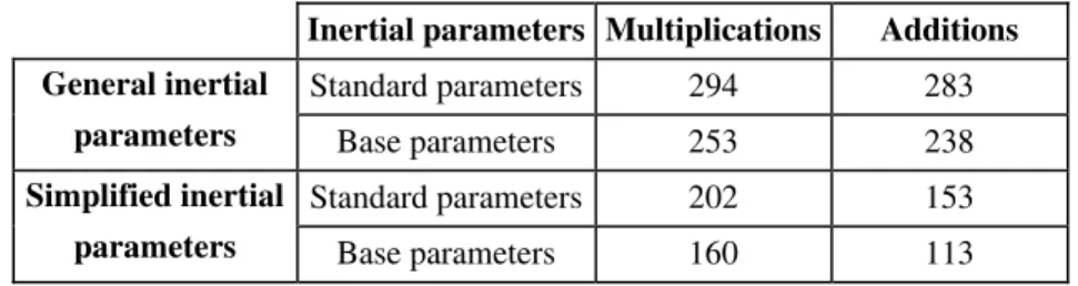
Table 7.6. shows the computational complexity of the inverse dynamic model for the Stäubli RX-90 robot using the customized Newton-Euler formulation. In Appendix 7, we give the dynamic model of the Stäubli RX-90 robot when using the base inertial parameters of Table 7.4, which takes into account the symmetry of the

links. The corresponding computational cost is 160 multiplications and 113 additions.

Table 7.6. Computational complexity of the inverse dynamic model

for the Stäubli RX-90 robot

Inertial parameters Multiplications Additions General inertial parameters Standard parameters 294 283 Base parameters 253 238 Simplified inertial parameters Standard parameters 202 153 Base parameters 160 113

7.6. Direct dynamic model

The computation of the direct dynamic model is employed to carry out simulations for the purpose of testing the robot performances and studying the synthesis of the control laws. During simulation, the dynamic equations are solved for the joint accelerations given the input torques and the current state of the robot (joint positions and velocities). Through integration of the joint accelerations, the robot trajectory is then determined. Although the simulation may be carried out off-line, it is interesting to have an efficient direct dynamic model to reduce the simulation time. In this section, we consider two methods: the first is based on using a specialized Newton-Euler inverse dynamic model and needs to compute the inverse of the inertia matrix A of the robot; the second method is based on a recursive Newton-Euler algorithm that does not explicitly use the matrix A and has a computational cost that varies linearly with the number of degrees of freedom of the robot.

7.6.1. Using the inverse dynamic model to solve the direct dynamic problem From equation [7.6], we can express the direct dynamic problem as the solution of the joint accelerations from the following equation:

A ..q = [ –H(q, q.)] [7.62]

where H contains the Coriolis, centrifugal, gravity, friction and external torques: H(q, q.) = C(q, q.) q. + Q + diag(q.)Fv + diag(sign(q.))Fc + JT fen

Although in practice we do not explicitly calculate the inverse of the matrix A, the solution of equation [7.95] is generally denoted by:

..

q = A-1 _{[ – H(q, q}._{)] [7.63]}

The computation of the direct dynamics can be broken down into three steps: the calculation of H(q, q.), the calculation of A, and the solution of the linear equation [7.62] for ..q.

The computational complexity of the first step is minimized by the use of a specialized version of the inverse dynamics algorithm in which the desired joint accelerations are zero [Walker 82]. By comparing equations [7.1] and [7.63], we deduce that H(q, q.) is equal to ifq = 0. ..

The inertia matrix can also be calculated one column at a time, using Newton-Euler inverse dynamic model [Walker 82]. From relation [7.62], we deduce that the ith _{column of A is equal to  if:}

..

q =u_i, q. = 0, g = 0, F_c= 0 (f_ej = 0, m_ej = 0 for j = 1,…, n) [7.64] where u_i is an (nx1) unit vector with 1 in the ith _{row and zeros elsewhere. Iterating} the procedure for i = 1,…, n leads to the construction of the entire inertia matrix.

To reduce the computational complexity of this algorithm, we can make use of the base inertial parameters and the customized symbolic techniques. Moreover, we can take advantage of the fact that the inertia matrix A is symmetric. A more efficient procedure for computing the inertia matrix using the concept of composite links is given in Appendix 8. Alternative efficient approaches for computing the inertia matrix based on the Lagrange formulation are proposed in [Megahed 82], [Renaud 85].

NOTE.– The nonlinear state equation of a robot follows from relation [7.62] as:













q. q.. =













q. A-1 _{[ – H(q, q}._)]  [7.65]

and the output equation is written as:

y = q or y = X(q) [7.66]

In this formulation, the state variables are given by [qT _q.T_]T_{, the equation y = q} gives the output vector in the joint space, and y = X(q) denotes the coordinates of the end-effector frame in the task space.

7.6.2. Recursive computation of the direct dynamic model

This method is based on the recursive Newton-Euler equations and does not use explicitly the inertia matrix of the robot [Armstrong 79], [Featherstone 83b], [Brandl 86]. The joint accelerations are obtained as a result of three recursive computations:

7.6.2.1 Algorithm of computation of the direct dynamic model

i) first forward recursive computations for j = 1, …, n: in this step, we compute the

screw transformation matrices j_{Sj-1, the link angular velocities} j_{j as well as} j_{j and} j_{j vectors, which represent the link accelerations and the link wrenches respectively} when..q= 0;

Using the screw notation and by combining equations [7.54] and [7.53], which give j_V._{j and} j_{.j, we obtain:}

j_V._{j =} j_Sj-1 j-1_V._{j-1 +} .._qjj_{aj +} j_{j [7.67]} where j_{aj is defined by equation [7.23b], and:}

j_{j =}

















j_Rj-1[j-1_{j-1 x (}j-1_{j-1 x} j-1_{Pj)] + 2j (}j_{j-1 x q}._jj_aj) –_j j_{j-1 x q}._j j_aj [7.68]

Equations [7.88], [7.89], [7.91] and [7.93], which represent the equilibrium equations of link j, can be combined as:

j_Ij j_V._{j =} j_{Fj –} j+1_ST j j+1Fj+1 + jj [7.69] where: j_{j = –} j_{Fej –}













j_{j x (}j_{j x} j_MSj) j_ j x (jIOjjj) [7.70] In equation [7.69], we use equation [2.34] to transform the dynamic wrench

ii) backward recursive computations for j = n, ..., 1: in this step we calculate the

elements H _j, j_J*

j , j*j, jKj , jj which express ..qj and Fj in terms of j-1

.

Vj-1 in the third recursive equations. These equations will be demonstrated in the next section.

For j = n, ..., 1, compute: Hj = (jaTj jI*j jaj+ Iaj) [7.71] j_{Kj =} j_I* j – jI*j jaj H-1j ja T j jI*j [7.72] j_ j = jKj jj + jI*j jaj Hj-1(j +jaTj j*j) – j*j [7.73] where (see equation 7.82)

 _{j = j} – Fsj sign(q.j) – Fvjq.j If j ≠ 1, calculate also: j-1_* j -1 = j-1*j -1 – jSTj-1jj [7.74] j-1_I* j -1 = j-1I*j -1 + jSj-1T jKj jSj-1 [7.75]

Note that these equations are initialized by j_I*

j = jIjand j*j = jj;

iii) second forward recursive computations. Since 0_V.

0 is composed of the linear and angular accelerations of the base that are assumed to be known (v.₀ = –g, .₀ = 0 for fixed base), the third recursive computation allows us to compute ..q_{j ,} j_v.

j and jFj (if needed) for j = 1… n. as follows :

j_V._{j-1,j =} j_Sj-1 j-1_V._{j-1 [7.76]} .. q_j = H-1_j [– j_aT j jI*j (j . Vj-1,j + jj) + j +jaTj j*j] [7.77] j_V._{j =} j_V._{j-1,j +} j_aj.._{qj +} j_{j [7.78]} j_{Fj =}













j_fj j_mj = jI * j j . Vj- j*j [7.79]

NOTES.–

– to reduce the number of operations of this algorithm, we can make use of the base inertial parameters and the customized symbolic technique. Thereby, the number of operations of the direct dynamic model for the Stäubli RX-90 robot is 889 multiplications and 653 additions [Khalil 97]. In the case of the use of simplified inertial parameters (Table 7.4), the computational cost becomes 637 multiplications and 423 additions;

– the computational complexity of this method is O(n), while the method requiring the inverse of the robot inertia matrix is of complexity O(n3_);

– from the numerical point of view, this method is more stable than the method requiring the inverse of the robot inertia matrix [Cloutier 95].

7.6.2.2 Demonstration of relations [7.67] and [7.68]

To illustrate the equations required, we detail the case when j = n and j = n – 1. By combining equations [7.67] and [7.69] for j = n, and since n+1_{Fn+1 = 0, we obtain:}

n_I n (nSn-1 n-1 . V_n-1 +..q_n n_a n + nn) = nFn+ nn [7.80] Since: j_aT j jFj = j – Iaj..qj [7.81] _{j = j} – F_sj sign(q._j) – F_vjq._j [7.82] multiplying equation [7.71] by n_aT

n and using equation [7.72], we deduce the joint acceleration of joint n: .. q_n = H-1_n (– n_aT n nIn (nSn-1 n-1 . V_n-1 + n_ n) + n +naTn nn) [7.83] where H_n is a scalar given as:

H_n = (n_a

nT nInnan+ Ian) [7.84]

Substituting for ..q_n from equation [7.83] into equation [7.82], we obtain the dynamic wrench n_F

n_{Fn =}













n_fn n_m n = n_Kn n_Sn-1n-1_V._{n-1 +} n_{n [7.85]} where: n_{Kn =} n_In– n_In n_anH-1 n naTnnIn [7.86] n_ n = nKn nn + nIn nanH-1n (n +naTn nn) – nn [7.87] We now have ..q_n and n_F

n in terms of n-1

.

Vn-1. Iterating the procedure for j = n – 1,

we obtain, from equation [7.79]:

n-1_In-1 n-1_V._n-1= n-1_Fn-1+ n_ST

n-1nFn+ n-1n-1 [7.88]

which can be rewritten using equation [7.67] as: n-1_I* n-1 (n-1Sn-2 n-2 . Vn-2 + ..qn-1 n-1an-1+ n-1n-1) = n-1Fn-1+ n-1*n-1 [7.89] where: n-1_I* n-1 = n-1In-1 + nSTn-1nKn nSn-1 [7.90] n-1_* n-1 = n-1n-1 – nSTn-1nn [7.91] Equation [7.90] has the same form as equation [7.83]. Consequently, we can express ..q_{n-1 and} n-1_{Fn-1in terms of} n-2_V._{n-2. Iterating this procedure for j = n – 2, …,}

1, we obtain ..q_j and j_F

j in terms of n-1

.

Vn-1 for for j = n – 1, ..., 1 using equations

[2.77] and [7.78] which are similar to [7.83] and [7.85]. 7.7. Conclusion

In this chapter, we have presented the dynamics of serial robots using Lagrange and Newton-Euler formulations that are linear in the inertial parameters. The Lagrange formulation allowed us to study the characteristics and properties of the dynamic model of robots, while the Newton-Euler was shown to be the most efficient for real time implementation. In order to increase the efficiency of the Newton-Euler algorithms, we have proposed the use of the base inertial parameters in a customized symbolic programming algorithm. The problem of computing the direct dynamic model for simulating the dynamics of robots has been treated using two methods; the first is based on the Newton-Euler inverse dynamic algorithm,

while the second is based on another Newton-Euler algorithm that does not require the computation of the robot inertia matrix.

We note that the inverse and direct dynamic algorithms using recursive Newton-Euler equations have been generalized to flexible robots [Boyer 98] and to systems with lumped elasticities [Khalil 00a].