Euclidean Revealed Preferences: Testing the Spatial Voting Model

Texte intégral

(1)2011s-49. Euclidean Revealed Preferences: Testing the Spatial Voting Model Marc Henry, Ismael Mourifié. Série Scientifique Scientific Series. Montréal Juin 2011. © 2011 Marc Henry, Ismael Mourifié. Tous droits réservés. All rights reserved. Reproduction partielle permise avec citation du document source, incluant la notice ©. Short sections may be quoted without explicit permission, if full credit, including © notice, is given to the source..

(2) CIRANO Le CIRANO est un organisme sans but lucratif constitué en vertu de la Loi des compagnies du Québec. Le financement de son infrastructure et de ses activités de recherche provient des cotisations de ses organisations-membres, d’une subvention d’infrastructure du Ministère du Développement économique et régional et de la Recherche, de même que des subventions et mandats obtenus par ses équipes de recherche. CIRANO is a private non-profit organization incorporated under the Québec Companies Act. Its infrastructure and research activities are funded through fees paid by member organizations, an infrastructure grant from the Ministère du Développement économique et régional et de la Recherche, and grants and research mandates obtained by its research teams. Les partenaires du CIRANO Partenaire majeur Ministère du Développement économique, de l’Innovation et de l’Exportation Partenaires corporatifs Autorité des marchés financiers Banque de développement du Canada Banque du Canada Banque Laurentienne du Canada Banque Nationale du Canada Banque Royale du Canada Banque Scotia Bell Canada BMO Groupe financier Caisse de dépôt et placement du Québec CSST Fédération des caisses Desjardins du Québec Financière Sun Life, Québec Gaz Métro Hydro-Québec Industrie Canada Investissements PSP Ministère des Finances du Québec Power Corporation du Canada Rio Tinto Alcan State Street Global Advisors Transat A.T. Ville de Montréal Partenaires universitaires École Polytechnique de Montréal HEC Montréal McGill University Université Concordia Université de Montréal Université de Sherbrooke Université du Québec Université du Québec à Montréal Université Laval Le CIRANO collabore avec de nombreux centres et chaires de recherche universitaires dont on peut consulter la liste sur son site web. Les cahiers de la série scientifique (CS) visent à rendre accessibles des résultats de recherche effectuée au CIRANO afin de susciter échanges et commentaires. Ces cahiers sont écrits dans le style des publications scientifiques. Les idées et les opinions émises sont sous l’unique responsabilité des auteurs et ne représentent pas nécessairement les positions du CIRANO ou de ses partenaires. This paper presents research carried out at CIRANO and aims at encouraging discussion and comment. The observations and viewpoints expressed are the sole responsibility of the authors. They do not necessarily represent positions of CIRANO or its partners.. ISSN 1198-8177. Partenaire financier.

(3) Euclidean Revealed Preferences: Testing the Spatial Voting Model * Marc Henry †, Ismael Mourifié ‡. Abstract In the spatial model of voting, voters choose the candidate closest to them in the ideological space. Recent work by (Degan and Merlo 2009) shows that it is falsifiable on the basis of individual voting data in multiple elections. We show how to tackle the fact that the model only partially identifies the distribution of voting profiles and we give a formal revealed preference test of the spatial voting model in 3 national elections in the US, and strongly reject the spatial model in all cases. We also construct confidence regions for partially identified voter characteristics in an augmented model with unobserved valence dimension, and identify the amount of voter heterogeneity necessary to reconcile the data with spatial preferences. Keywords: revealed preference, partial identification, elliptic preferences, voting behaviour. Codes JEL: C19, D72. *. Date: The present version is of May 17, 2011. Financial support from SSHRC Grant 410-2010-242 is gratefully acknowledged. The authors are also grateful to the co-editor Thierry Magnac, three anonymous referees, Russell Davidson, Romuald Méango, Aureo de Paula, Yves Sprumont, Bernard Salanié, Étienne de Villemeur and participants at the Montreal Conference on Revealed Preferences and Partial Identification and the Penn State econometrics seminar for helpful discussions. The usual disclaimer applies. † Département de sciences économiques, Université de Montréal, C.P. 6128, succursale Centre-ville, Montréal QC, H3C 3J7, Canada. Tel: 1 (514) 343-2404. Fax: 1 (514) 343-7221. Email: marc.henry@umontreal.ca ‡ Université de Montréal..

(4) ´ MARC HENRY AND ISMAEL MOURIFIE. 2. Introduction The analysis of voting decisions is an integral part of the revealed preference theory of non-market interactions. A dominant framework in the analysis of voting data is the spatial theory of voting of (Hotelling 1929) and (Downs 1957), which characterizes voters and candidates in an election by their positions in a common ideological space and postulates that voters choose candidates closest to them in that space (see (Hinich and Munger 1997) and (Poole 2005) for accounts of the theory). Two fundamental questions arise regarding the empirical content of this theory.. (1) Are the distribution of voter ideological positions (hence voter preferences) identified on the basis of voting choices? (2) Can the fundamental behavioral assumption of the spatial theory be rejected on the basis of voting data?. Following the work of (Heckman and Snyder 1997) and (Poole and Rosenthal 1997), data on the position of candidates in a two-dimensional ideological space are now widely available (see also (Poole 2005) and references therein). Hence the first question can be reformulated in the following way: does the maintained assumption of spatial voting allow the identification of voter positions in the ideological space on the basis of the knowledge of candidate positions and aggregate voting outcomes? This question is answered affirmatively by (Merlo and de Paula 2009) who also provide a nonparametric estimation strategy with data on repeated elections. The second question is tackled in different guises by (Bogomolnaia and Laslier 2007), (Degan and Merlo 2009) and (Kalandrakis 2010). (Bogomolnaia and Laslier 2007) find the minimal dimension for the ideological space such that voter preference orderings over a finite number of candidates can be represented by spatial utility functions. (Kalandrakis 2010) derives testable restrictions on the positions of voters’ ideal points based on a finite number of binary voting choices, when the positions of the alternatives are known. (Degan and.

(5) EUCLIDEAN REVEALED PREFERENCES. 3. Merlo 2009) establish conditions for the falsifiability of the spatial model in the context of multiple elections, individual voting profile data and observable candidate positions. Falsifiability then derives from the multiplicity of elections; in a single election, a vote for candidate j is compatible with the voter’s ideal point lying in the Voronoi cell of candidate j’s position (i.e. all points in the space for whom j is closest among all alternatives). With multiple elections, a voting profile is compatible with the voter belonging to the intersection of the Voronoi cells of respective candidates chosen in that voting profile. When the number of elections is strictly larger than the dimension of the ideological space, some such intersections are empty and the spatial model is falsifiable. Based on this result, we first provide an econometric methodology to formally test the hypothesis of spatial voting based on observed individual voting profiles from multiple elections, where the ideological position of candidates are known. The main difficulty in setting up a test of the spatial voting model is that the model does not pin down the data generating process for the voting profiles. This is in sharp contrast with the literature on compatibility of discrete choice probabilities and stochastic utility maximization. (Daly and Zachary 1979) and (McFadden 1979) give necessary and sufficient conditions for a discrete choice distribution to be compatible with the maximization of an additively separable random utility. See also (Borsch-Supan 1990) and (Koning and Ridder 2003). The compatibility conditions rely crucially on the coherency of the model, in the sense of (Heckman 1978) and (Gouriéroux, Laffont, and Monfort 1980), and identifiability of its components. We show that in the present context, despite lack of identification, the null hypothesis of compatibility between the voting data and the spatial model can still be formally tested with an appeal to partial identification techniques recently developed in (Galichon and Henry 2011). This partial identification approach to revealed preference testing relates our work directly to (Blundell, Browning, and Crawford 2008), (Hoderlein and Stoye 2009) and, even more closely (Kawai and Watanabe 2010). The latter partially identify preference parameters in a voting model in which a.

(6) 4. ´ MARC HENRY AND ISMAEL MOURIFIE. fraction of voters incorporate strategic considerations in their voting decisions. A partially identified setting also arises in (Hoderlein and Stoye 2009) who provide a test of WARP based on consumption data from repeated cross sections of heterogeneous consumers. Finally, (Blundell, Browning, and Crawford 2008) also provide empirical implications of revealed preference axioms in the forms of bounds on demand responses. We test spatial voting in US National elections for years 2000, 2004, and 2008 and the whole data combined. In all three elections, we reject the hypothesis that voters have elliptic preferences over candidates. That is to say, we reject the spatial voting model with heterogeneity of unknown form, both in voter bliss points and in the distances characterizing preferences. This brings new striking evidence to bear on the debate over the adequacy of the spatial voting model in explaining stylized facts on the positioning of political party platforms, and the convergence to the center implied by median voter results (see (Zakharov 2008) for an excellent account). Former empirical analysis and tests of the spatial voting model were conducted assuming knowledge of voter ideological positions (see (Alvarez and Nagler 1998), (Jeong 2008) and references therein). The latter is a reasonable assumption, when analyzing roll call voting in the House and the Senate, but much less so, when analyzing voter behavior in general elections. Another substantial distinction with roll call voting is the coexistence and competition of two voting logics in general elections, ideology versus performance. The spatial model describes voters’ preferences over the candidate’s program, whereas preferences over the candidate herself, involving charisma, experience and competence, are typically captured with an additive non spatial term in the utility, generally called valence. A fundamental difference between the valence dimensions and the dimensions of the ideological space is that preferences are satiated relative to the latter only. The spatial model is augmented with a valence dimension in (Ansolabehere and Snyder 2000) and.

(7) EUCLIDEAN REVEALED PREFERENCES. 5. (Groseclose 2001). (Azrieli 2009) axiomatizes the model and (Schofield 2007) shows that incorporating the valence dimension leads to equilibria, where party platforms do not all converge to the center of the electoral distribution. As in the problem of testing the validity of the spatial model, the problem of estimating and testing valence specifications of the spatial model is complicated by the fact that voter’s ideal points are unobserved and the model only partially identifies the distribution of voting profiles. We show how to construct confidence regions for the partial effect of distance to ideal point and of valence characteristics in the utility specification. Of particular empirical relevance are the spatial preference parameter configurations compatible with the smallest values of valence dispersion. These can be interpreted as estimates of the spatial preference parameters that best rationalize the data. A notable finding is that voter differ from candidates in their perception of the relevant ideological dimensions and that the liberal-conservative axis of the standard ideological space dominates the social issues axis in voter preferences. This opens the possibility for parties to gain vote shares by rebalancing political platforms. The rest of this paper is organized as follows. In the Section 1 we characterize the empirical content of the spatial model of voting. In Section 2, we introduce valence. The data is described in Section 3 and the empirical results in Section 4. The last section concludes.. 1. Empirical content of the spatial voting model 1.1. Analytical framework. The spatial model of voting postulates a common ideological space Y ⊆ Rk , where k is the number of ideological dimensions. Voters face m > k simultaneous elections, each indexed by e ∈ {1, ..., m}. In election e, each voter chooses exactly one candidate e j e ∈ J e = {1, . . . , q e } among the q e candidates competing in election e. All candidates j ∈ ∪m e=1 J.

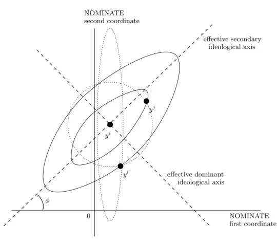
(8) ´ MARC HENRY AND ISMAEL MOURIFIE. 6. are characterized by their position y j in the ideological space, which is observed by the voters and the analyst. In the rest of this work, we shall consider only two-candidate elections, hence q e = 2. Because of its elegance, simplicity and interpretability, the spatial voting model has dominated a large section of the literature on the analysis of voting choices. An excellent account can be found in (Zakharov 2008). Following the principal component analysis of roll call voting in the US Congress, the two-dimensional NOMINATE Common Space (Poole and Rosenthal 1997) has become a staple of empirical work on the issue. Ideological positions of members of Congress are estimated on the unit square of a two-dimensional space, the first axis of which is usually interpreted as the liberal-conservative axis, measuring economic conservatism, and the second axis of which is usually interpreted as measuring position on social issues. Given the prevalence of this two-dimensional spatial voting model, we will concentrate on the case k = 2 in the rest of this work. Voters are said to have Euclidean preference (or to “vote ideologically”) if their preferences are satiated at a bliss point y i for voter i in the ideological space and if they maximize a utility function, which is decreasing in the Euclidean distance between their bliss point and the position y j of the chosen candidate.. Definition 1 (Euclidean preferences). Voter i ∈ I has Euclidean preferences (“votes ideologically”) if there exists y i ∈ Y such that voter i chooses to vote for candidate j in each election e, denoted 0. vei = j, if and only if y j minimizes distance d(y i , y; ω) among y j , j 0 ∈ J e , where ω = (ω1 , ω2 )0 , ω22 < ω1 and µ d(y, y 0 ; ω) = (y − y 0 )t. 1 ω2. ω2 ω1. ¶ (y − y 0 ).. Figure 1 shows the elliptic indifference curves for a voter, whose ideological bliss point is y i and whose utility when candidate with position y j is elected is a negative non increasing function of d(y i , y j ; ω). The dotted circle represents an indifference curve for voter i when ω1 = 1 and ω2 = 0,.

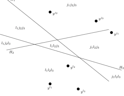
(9) EUCLIDEAN REVEALED PREFERENCES. 7. i.e. when the space of reference for candidate coordinates is the effective ideological space for the voter. Note that candidates y j and y l are both on the circle, and hence are indifferent. The dotted vertical ellipse represents the indifference curve for voter i when ω2 = 0 and ω1 < 1. In that case, the main axes are still the effective ideological dimensions, but in the given units of measurements, the horizontal axis is dominant in the sense that y l , closer to y i in the horizontal dimension, is preferred to y j , closer to y i in the vertical dimension. When ω2 6= 0, the ideological space is different from the reference space. y j is now preferred to y l .. i ) the voting profile of voter i, i.e the 1.2. Falsifiability of the model. Denoting v i = (v1i , ..., vm. collection of candidates voter i chooses in elections e = 1, ..., m, the hypothesis that voters have Euclidean preferences is falsifiable if there exist at least one voting profile ve, which cannot be rationalized by the maximization of Euclidean preferences in each election.. Example 1. In figure 2, we illustrate a case with two ideological dimensions and 2 simultaneous elections with 2 candidates each. The black dots represent candidate positions, y j1 and y l1 in election 1 and y j2 and y l2 in election 2. The lines He , e = 1, 2 separate the ideological space into the half-space, where voters vote for candidate je and the half-space, where voters vote for candidate le . The intersection of the half-space, where voters vote for j1 in the first election, say and the halfspace, where voters vote for l2 in the second elections is denoted j1 l2 in the figure. All four possible voting profiles are rationalizable by the maximization of Euclidean preferences, hence the hypothesis is not falsifiable.. Example 2. In figure 3, we illustrate the case with 2 ideological dimensions and 3 simultaneous elections, with = 2 candidates each. In addition to the half-spaces in example 1, H3 separates the ideological space in two regions, one, where voters prefer (are closer to) candidate j3 and one, where voters prefer (are closer to) candidate l3 . The intersection of three half-spaces corresponds.

(10) 8. ´ MARC HENRY AND ISMAEL MOURIFIE. to a particular voting profile. For any configuration of candidate positions such that y j 6= y l when j 6= l, there is exactly one voting profile which is incompatible with Euclidean preference, hence the hypothesis is falsifiable. In figure 3, the half-spaces of voters, who vote for j1 in election 1, for j2 in election 2 and for l3 in election 3 have empty intersection. Hence, voting profile j1 j2 l3 is incompatible with spatial voting.. More generally, (Degan and Merlo 2009) show that for two candidate elections, falsifiability is equivalent to m > k. In a small data exploration on US National elections, where voters are faced with m = 3 simultaneous elections (presidential, senate and house) and individual voting profiles and candidate ideological positions in R2 are observed, (Degan and Merlo 2009) find evidence of violations of ideological voting as defined in Definition 1 with ω1 = 1 and ω2 = 0 constant across voters. In the data set that we consider, with the US 2000, 2004 and 2008 elections, we report incidence of violations of the spatial model with no heterogeneity in Table 4. In order to evaluate the statistical significance of these violations and examine alternative specifications, some form of voter heterogeneity needs to be introduced in the utility specification. Unobserved heterogeneity may be entertained within the spatial model in the form of voter specific distance d(., .; ω) as we describe in the next section. It may also take the form of a non spatial random utility term, when allowing for voters’ response to non ideological characteristics of the candidate. We defer the discussion of the latter form of voter heterogeneity to Section 2 below. 1.3. Unobserved preference heterogeneity. Preference heterogeneity may be entertained within the framework of the spatial voting model by assuming that voters may differ in their perception of the relevant ideological dimensions. That is to say, the distance d(., .; ω) in the spatial utility function may be voter specific. Thus the requirement that voters have Euclidean preferences according to definition 1 is equivalent to a requirement that all voters have outward decreasing elliptic preferences in that each voter i with position y i chooses candidate to minimize d(y i , y j ; ω i ), where.

(11) EUCLIDEAN REVEALED PREFERENCES. 9. ω i is voter specific. To conduct a revealed preference test of this assumption of elliptic preference maximization, we need to characterize the empirical content of the assumption as follows. Let X denote the set of observable variables, which includes the positions of all candidates in the elections. A given voter with bliss point (position in the ideological space) y and preference parameter ω characterizing the shape of her indifference curves is facing m = k + 1 = 3 elections (recalling that k = 2 is the dimension of the ideological space) characterized by the vector X of positions of all candidates. Given (y, ω, X), the resulting voting profile v is uniquely determined by the voting model as long as assumptions on the distribution of candidates rule out ties. Denote the unique implied voting profile v = g(ω|X, y), which is the profile of choices of candidates je 0. such that y je minimizes d(y, y je ; ω) among candidates je0 ∈ {je , le } in each election e. For instance, in example 2, g(ω|X, y) = l1 l2 j3 when y belongs to the central triangle. However, the position y of voters is unobservable, hence all that utility maximization predicts is that v lies within the set of compatible voting profiles, which depends on the positions of candidates X and the realization ω of preference heterogeneity. For instance, in example 2, the model only tells us that v lies in {j1 j2 j3 , j1 l2 j3 , j1 l2 l3 , l1 j2 j3 , l1 j2 l3 , l1 l2 j3 , l1 l2 l3 }. We denote G(ω|X) this set of compatible voting profiles, i.e., G(ω|X) =. S y. g(ω|X, y). The model predicts the following bound on the probability of. voting profile being V = v:. P(V = v|X) = P(g(ω|X, y) = v|X) ≤ P(v ∈ G(ω|X)|X),. since the only model prediction is g(ω|X, y) ∈ G(ω|X) for any y in the ideological space. Similarly, for any subset B of the set of all 2m possible voting profiles, the model predicts the following bound on the probability of the voting profile V belonging to B.. P(V ∈ B|X) ≤ P(G(ω|X) ∩ B 6= ∅|X).. [EC].

(12) 10. ´ MARC HENRY AND ISMAEL MOURIFIE. The inequalities above specify a set of bounds on the distribution of unobserved heterogeneity. As shown above, if voters’ choices are compatible with spatial preferences with heterogeneity, the inequalities in [EC] are necessarily satisfied. Conversely, if the inequalities in [EC] are satisfied, then voters’ choices can be rationalized by spatial preferences with heterogeneity. In that precise sense, the inequalities in [EC] define sharp bounds on the distribution of unobserved heterogeneity. The converse statement is a corollary of Theorem 1 in (Galichon and Henry 2011) (see also (Beresteanu, Molchanov, and Molinari 2011)). One way to gain insight into the proof of this result is to characterize rationalizability of voters’ choices by spatial preferences as the existence of an assignment of voting profiles v to unobserved heterogeneity values ω satisfying the constraints v ∈ G(ω|X). By the Marriage Lemma, such an assignment exists if and only if there is no over demanded set of ω’s, which in the present setting means there is no subset B of voting profiles such that P(B|X) > P(G(ω|X) ∩ B 6= ∅|X). The discussion above can be summarized in the following theorem, which gives the characterization of the empirical content of the model.. Theorem 1 (Empirical content). The empirical content of the spatial voting model is characterized by the inequalities [EC] for each subset B of the set of voting profiles.. Theorem 1 tells us that a test of the spatial voting model with heterogeneity in the shape of the voters’ indifference curves, i.e., in ω, is equivalent to testing that the inequalities [EC] hold. Letting the distribution of unobserved heterogeneity ω be characterized by the parameter vector θ, we consider the set ΘI (possibly empty) of values of θ, such that [EC] hold, noting that the right-hand side of [EC] depends on the distribution of ω, hence on θ. ΘI is called the identified set.. Definition 2. (Identified set) We call identified set ΘI the set of parameter values such that the moment inequalities in [EC] hold..

(13) EUCLIDEAN REVEALED PREFERENCES. 11. By theorem 1, ΘI is exactly the set of parameters θ such that the spatial voting model with heterogeneity is not rejected. ΘI is sometimes called sharp identified set to emphasize the fact that all values of θ in ΘI are observationally equivalent: no value in ΘI can be rejected on the basis of the information contained in the spatial model and the true distribution of voting profiles. As a result, a test of the inequalities of Theorem 1 is a classical revealed preference test of the spatial voting model. The way we implement the test is to construct a confidence region for the identified set, using the methodology proposed in (Henry, Méango, and Queyranne 2010) and described in detail in Appendix A. In the data set described in Section 3, we find a 99% confidence region for the identified set ΘI to be empty, hence we reject the spatial voting model specification with distance heterogeneity at the 99% level of significance (see Section 4 for details). In other words, the data cannot be rationalized by a model with heterogenous elliptic preferences.. 2. Introducing valence The rejection of the spatial model leads to the consideration of a non spatial component in preferences. As mentioned in the introduction, there is a large literature in political science that attempts to reconcile voting models with observed (non converging) distributions of political party platforms by combining two logics of voting in voter preferences, the logic of ideology, in a spatial term, and the logic of performance, in a non spatial non satiated valence term. We now adopt this approach in our empirical investigation of the determinants of voting choices. The specification generally considered in the literature is the following: voter i maximizes utility Ui (j) = −d(y i , y j ; ω)2 + ²ji. (2.1). in each election over j ∈ J e candidates. The valence term E = (²ji 1 , ²li1 , . . . , ²ji m , ²lim ) is independently distributed conditionally on X = (y j1 , y l1 , y j2 , y l2 , y j3 , y l3 ). Let the distribution of the valence term be parameterized with parameter θ..

(14) ´ MARC HENRY AND ISMAEL MOURIFIE. 12. As in the case of heterogeneity in the distance characterizing preferences in Section 1, we denote by G(²|X; ω) the set of compatible profiles for a given realization ² of unobserved valence heterogeneity. The same reasoning applies to show that the inequalities P(V ∈ B|X) ≤ P(G(²|X; ω) ∩ B 6= ∅|X; θ). [ECval]. for each subset B of voting profiles, characterize the empirical content of the spatial model with valence heterogeneity (note that now ² is the random unobserved heterogeneity, whereas ω is treated as a deterministic parameter vector). The characterization of the empirical content of the model in [ECval] still involves a large number of inequalities, namely up to one for each subset B of the set V m of voting profiles. It turns out that in the case of valence heterogeneity, we can achieve a dramatic dimension reduction to 2 inequalities. First we show the following lemma.. Lemma 1 (Incompatible profiles). Let m = k + 1 elections with 2 candidates in each election, then for almost all X, there is a pair of profiles v(X) and v(X) such that for all ², Gc (²|X; ω) = {v(X)} or Gc (²|X; ω) = {v(X)}.. In other words, for a given X characterizing the positions of all candidates, there is exactly one voting profile incompatible with Euclidean preferences and it belongs to a pair {v(X), v(X)}. This pair is independent of ², so that for different values of unobserved heterogeneity ², the unique incompatible profile can only take value v(X) or v(X). In example 2 and figure 3, the two profiles that are potentially incompatible with spatial voting are profiles l1 l2 j3 and j1 j2 l3 . The formal proof is given in the appendix, but it is very easy to understand its heuristics in figure 3: j1 j2 l3 is the only incompatible profile and l1 l2 j3 is the only profile with compact support, which is compatible with spatial voting. The slopes of separating hyperplanes are independent of ². Hence non compact profile supports cannot disappear, and the only profile that can disappear when ² shifts the location of the lines in the figure is l1 l2 j3 . The latter disappears and is replaced by j1 j2 l3 in any of the.

(15) EUCLIDEAN REVEALED PREFERENCES. 13. following three cases: H1 moves sufficiently to the left, H2 moves sufficiently to the right or H3 moves sufficiently to the right. We are now in a position to show our simple characterization of the empirical content of the model.. Theorem 2 (Empirical content of model with valence). The empirical content of the spatial voting model is characterized by exactly 2 inequalities P(v(X)|X) ≤ P(v(X) ∈ G(²|X; ω)|X; θ) and P(v(X)|X) ≤ P(v(X) ∈ G(²|X; ω)|X; θ).. (2.2). In other words, if the two inequalities are satisfied, then all inequalities in [ECval] are satisfied and the spatial model with valence heterogeneity is compatible with the true voting profile distribution. Conversely, if for some X, one of these two inequalities is violated, then the true voting distribution is incompatible with the spatial voting model with valence heterogeneity. We are interested in the set ΞI of parameter values ξ = (ω, θ) of the model (possibly empty) such that (2.2) holds. This set is the identified set in the model with valence heterogeneity. Our goal is to build a confidence region of asymptotic level cl for the identified set which is defined as a ˆ satisfying P(ΞI ⊆ Ξ) ˆ > cl asymptotically. The methodology derived from (Henry, Méango, region Ξ and Queyranne 2010) is detailed in appendix A, where a step-by-step account of the procedure is given. The procedure involves few, relatively simple steps and is computationally efficient. Once the ˆ is obtained, we can directly test specifications of the spatial model at the same confidence region Ξ ˆ is a set of values of the parameter vector ξ that are not rejected. level of significance. Recall that Ξ Suppose for illustration purposes, that ² is normal with mean zero and variance σ 2 . Suppose, ˆ does not contain any value of ξ with σ < 2, then σ 2 = 2 is a lower moreover that the region Ξ bound on the variance of unobserved valence necessary to rationalize the data with model (2.1). ˆ does not contain any value of ξ with (ω1 , ω2 ) = (1, 0), then the Suppose further that the region Ξ.

(16) ´ MARC HENRY AND ISMAEL MOURIFIE. 14. ˆ we always have ω2 > 0 and ω1 > 1, we spatial model with no distance distortion is rejected. If in Ξ can reject the hypothesis that the NOMINATE Common Space first coordinate (liberal-conservative axis) matters more to voters than the second coordinate (social issues). The partial identification approach adopted here is particularly well suited to the revealed preference problem at hand. Indeed, we wish to test to what extent the spatial model rationalizes the data. We have no information about the position of voters in the ideological space, hence it is undesirable to predicate rejection of the spatial model on ad-hoc assumptions on the latter. This would be the case, if we parameterized the distribution of voter positions and valence heterogeneity, imposed additional restrictions for identification of this nonlinear model, estimated with maximum likelihood and tested for the presence of unobserved heterogeneity with a version of (Chesher 1984).1. 3. Data Data are drawn from the following sources. The candidate positions are drawn from the Poole and Rosenthal NOMINATE Common Space data set2 ((Poole and Rosenthal 1997), (Poole 2005)), which gives the position of candidates on a two dimensional ideological space based on individual roll call voting of members of Congress. Only candidates who have held office are included in the data set. A fundamental assumption here is that voters observe the true ideological position of all candidates, whereas the econometrician only observes positions of candidates included in the NOMINATE Common Space data set. Each candidate that has not held office is assigned the position among all candidates in his party and district, which is most favorable to the hypothesis of spatial voting, to ensure that rejection of the model is not driven by missing data issues. This. 1. We are grateful to the co-editor Thierry Magnac for this suggestion.. 2. Available at http://voteview.com.

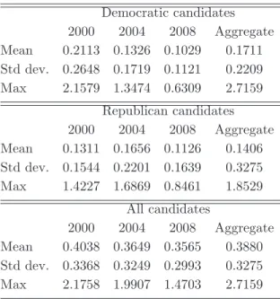
(17) EUCLIDEAN REVEALED PREFERENCES. 15. is done by choosing the position, which minimizes the number of voters in the district, who choose one of the pair of forbidden profiles {v(X), v(X)}. As for voting choices, they are obtained from the American National Elections Study (ANES), which represents the best and most widely used source of individual-level data on electoral participation and voting in United States3. For each election year, ANES contains individual voting decisions in presidential and congressional elections of a nationally representative sample of the voting age population. In addition, the ANES contains information on the congressional district where each individual resides, the identity of the Democratic and the Republican candidate competing for election in his or her congressional district, and, in the event that a Senate election is also occurring in his or her state, the identity of the candidates competing in the Senate race. For each election we consider a sub-sample, which contains only voters, who vote in the three simultaneous elections. Hence in any district h = 1, ..., 435 in state s = 1, ..., 50, a voter i is facing three simultaneous elections. As in (Degan and Merlo 2009), we match each voter in the ANES sample with the position of the presidential, senate and house candidates. We consider election years 2000, 2004 and 2008. 3.1. Candidate positions. Summary statistics on the distribution of candidate positions on the NOMINATE Common Space are described in Tables 2 and 3. Table 2 shows that democratic candidates are somewhat more dispersed than republican candidates in election year 2000, whereas republican candidates are somewhat more dispersed in election years 2004 and 2008. The overall dispersion is about twice as large as within party dispersion, but significantly smaller than between party dispersion, as shown in the top half of Table 3. The 0 in the latter table indicates that in election year 2000, one of the republican candidates shared their ideological position with one of the democratic candidates, indicating that they may have had an identical roll call voting record. The bottom half of Table 3 shows that the dispersion of elected candidates is greater than within 3. The ANES is available on-line at http://www.electionstudies.org/.

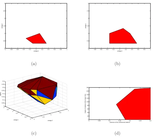
(18) 16. ´ MARC HENRY AND ISMAEL MOURIFIE. party dispersion, but smaller than the overall dispersion of candidates. On the first axis, sometimes called liberal-conservative axis, democratic and republican candidates are clearly separated, in the sense that for every election year as well as for the aggregate data, mean ± two standard deviations confidence intervals for democratic and republican candidates are disjoint. This feature is also very visible on the scatter plots of figure 4. On the second axis (also referred to as the social issues axis), however, the distributions of democratic and republic candidates are not clearly distinguishable. 3.2. Voting profiles. The distributions of voting profiles for elections years 2000 to 2008 are given in Table 1. A large majority of voters choose candidates from the same party in all three elections (75% in 2000, 76% in 2004 and 78% in 2008). Otherwise, no clear pattern arises among the remaining voting profiles.. 4. Empirical results 4.1. Distance heterogeneity. We considered a normal specification for ω2 with mean µ2 and variance σ22 and a log-normal specification for ω1 with mean µ1 and variance σ12 . ω1 and ω2 were assumed independent. We restricted the parameter space to (µ1 , µ2 ) ∈ [−5, 5]×[0, 10] and (σ12 , σ22 ) ∈ [0, 13]2 . The 99% level confidence region for the parameter vector (µ1 , µ2 , σ12 , σ22 ) is empty, so that the spatial voting model with distance heterogeneity is rejected at the 99% level of significance. We conclude that voters’ choices cannot be rationalized by spatial voting, even if we let the shape of the indifference ellipses be voter specific. 4.2. Valence heterogeneity. We considered two parametric specification for the valence term ² in specification 2.1. We first modeled E = (²j1 , ²l1 , ²j2 , ²l2 , ²j3 , ²l3 ) as a vector of independent mean zero binary variables taking values η and −η. Some features of the resulting confidence regions are given in figure 5 for the aggregate data, and results from individual elections are available on request. We then considered the specification, where E is a vector of independent normal variables with mean.

(19) EUCLIDEAN REVEALED PREFERENCES. 17. zero and variance σ 2 . Some features of the resulting confidence regions are given in figure 6 for the aggregate data. Figure 5(c) shows the 3-dimensional confidence region for the parameters of the spatial model 2.1 (ω, η). It is a 95% confidence region for the set of values of the parameter vector under which the spatial model is valid. Figures 5(a) and (b) show the effect of an increase in the admissible valence dispersion on the set of rationalizable distance distortions ω. The pure Euclidean model with ω2 = 0 and ω1 = 1 (such that indifference curves are circles) lies outside the cut in confidence region in figure 5(a), so it is not rationalizable, but it lies inside the cut in figure 5(b), so it becomes rationalizable for this higher level of admissible valence dispersion. The minimum value of η in the region is 0.128. This indicates that the spatial model can only be rationalized by adding a non ideological term in the utility of magnitude at least 0.128. This is to be compared with the distribution of squared distances between candidates in Table 2. The minimum valence needed to rationalize the valence-augmented spatial model is of the order of the mean of squared distances between democratic candidates, half the mean of squared distances between all candidates and a quarter of the mean of squared distances between democratic and republican candidates. Moreover, for that minimal non spatial utility term, the model can only be rationalized for a specific distance distortion, namely ω = (ω1 , ω2 ) = (0.333, −0.111). This corresponds to a much greater emphasis on the liberal-conservative axis than on the social axis. This can be seen more clearly on figure 5(d) which shows the tilt of the major axis of the elliptic indifference curves of voters compatible with the minimum valence magnitude. The value is close to 100 degrees, which indicates a situation similar to the dotted vertical ellipse of figure 1. The NOMINATE Common Space is shared by voters, except that greater importance is given to changes on the liberal-conservative axis. We see on figure 5(d) that the tilt of the indifference ellipses remains between 45 and 135 degrees for any value of the non ideological disturbance η below 0.222. So the conclusion on the relative weights of each axis remains..

(20) 18. ´ MARC HENRY AND ISMAEL MOURIFIE. In case of normal specification of the valence term, the 95% confidence region for the set of parameters (ω, σ) for which the valence-augmented spatial model is rationalizable is plotted in figure 6(c). The minimal standard deviation needed to rationalize the valence-augmented spatial model is 0.133. The corresponding indifference curves are ellipses with major axis titled at 100 degrees again, so that similar conclusions apply. The liberal-conservative axis remains dominant for all values of the valence standard deviation below 0.178. Again, figures 6(a) and (b) show the effect of an increase in the admissible valence dispersion on the set of rationalizable distance distortions ω. The pure Euclidean model with ω2 = 0 and ω1 = 1 (such that indifference curves are circles) lies outside the cut in confidence region in figure 6(a), so it is not rationalizable, but it lies inside the cut in figure 6(b), so it becomes rationalizable for this higher level of admissible valence dispersion. As seen on Table 5, those conclusions remain for data on individual elections, with however a clear trend towards the spatial model, as the lowest valence term necessary to rationalize the data drops from 0.119 in the 2000 elections, to 0.089 in the 2004 election and finally 0.059 in the 2008 elections. Overall results strongly support the hypothesis that voters’ choices are driven by a combination of ideological and competence considerations, as the magnitude of valence dispersion needed to rationalize voter choices is very close to the mean of the distribution of squared ideological distances between candidates from the same party and a fifth of the mean of squared ideological distances between candidates of opposing parties. Results also strongly support the hypothesis that voters give more weight to the liberal-conservative axis in the NOMINATE Common Space. The estimated distance distortion gives candidates a direction in which to rebalance their political program in order to increase their vote share. However, results do not support the hypothesis that the social issues axis is irrelevant in voters’ decisions. Indeed, the minimum valence dispersion needed to rationalize voters’ choices with a single ideological dimension (liberal-conservative axis alone, namely ω1 = ω2 = 0) is.

(21) EUCLIDEAN REVEALED PREFERENCES. 19. 50% larger than the dispersion needed to rationalize voters’ choices with two ideological dimensions (see Table 5).. Conclusion We have considered the spatial model of voting and provided a methodology for conducting revealed preference tests of spatial preferences. Falsifiability of the model is driven by the existence of voting profiles in multiple elections that are incompatible with maximization of spatial preferences in each election. The main difficulty in testing the hypothesis of spatial voting is that the latter only specifies a set of voting profiles compatible with spatial voting, and hence only partially identifies the distribution of voting profiles. It is shown here how to circumvent this fundamental characteristic of revealed preference tests with an appeal to recent results in partial identification. The hypothesis of spatial preferences is strongly rejected in a sample of voting profiles from three US elections, and confidence regions are constructed for the set of parameters compatible with the spatial voting model augmented with an unobserved non spatial component. A robust finding from those confidence regions is that the ideological dimension generally associated with economic conservatism dominates the dimension associated with social issues. The methodology is currently being extended to the estimation of revealed spatial preferences over competing characteristics in social networks with homophily, to complement work in (Christakis, Fowler, Imbens, and Kalyanaraman 2010), (Galichon and Salanié 2010) and (Chiappori, Gandhi, Salanié, and Salanié 2009).. Appendix A. Inference methodology The methodology is detailed for inference on the identified set ΞI in case of valence heterogeneity. It also applies to inference on the identified set ΘI in case of distance heterogeneity with a trivial.

(22) ´ MARC HENRY AND ISMAEL MOURIFIE. 20. change of notation, ΘI for ΞI and ω for ², and replacing the two inequalities of Theorem 2 by the inequalities in [EC]. ˆ such that the true identified set ΞI is We are interested in constructing a random region Ξ ˆ with at least probability cl. Given the sample of observations ((V1 , X1 ), . . . , (Vn , Xn )) contained in Ξ for a sample of n voters, we construct data dependent functions P (.|x) such that the following statement is true with probability tending to no less than cl: P (˜ v |Xi ) ≤ P (˜ v |Xi ) for all Xi , ˆ = {ξ = (ω, θ) | P (˜ v |Xi ) ≤ P(˜ v ∈ and v˜ ∈ {¯ v (Xi ), v(Xi )}. Once this is achieved, the region Ξ G(²|Xi , ω)|Xi ; θ), i = 1, . . . , n, v˜(X) ∈ {¯ v (X), v(X)}} satisfies the required conditions: indeed, if ξ ∈ ΞI , ξ satisfies (2.2), so with probability no less than cl, it also satisfies P (˜ v |Xi ) ≤ P(˜ v ∈ ˆ The confidence region G(²|Xi , ω)|Xi ; θ), i = 1, . . . , n, v˜(X) ∈ {¯ v (X), v(X)}, hence it belongs to Ξ. is computed by checking every parameter value ξ = (ω1 , ω2 , θ) on a regular grid of 106 points. There remains to explain how P(˜ v ∈ G(²|Xi , ω)|Xi ; θ) and P (.|Xi ) are computed.. A.1. Computation of P(˜ v ∈ G(²|Xi , ω)|Xi ; θ): For each value of Xi , i = 1, . . . , n and ξ = (ω, θ) on the grid, draw N = 999 values of valence ²l , l = 1, . . . , N . For each ²l , check whether v˜ ∈ G(²|Xi , ω) as in Section A.2. Approximate P(˜ v ∈ G(²|Xi , ω)|Xi ; θ) with the Monte Carlo probability (1/N ). P l=1,...,N. 1{˜ v ∈ G(²l |Xi , ω)}.. A.2. Checking whether v˜ ∈ G(²|Xi , ω): In election e with candidates je and le , voter with position y and valence perception E will choose candidate je if −d(y, y je ; ω)2 +²je > −d(y, y le ; ω)2 +²le which is equivalent to y·ω (y le −y je ) > 21 (ky je k2ω −ky le k2ω +²le −²je ), where “a·ω b” denotes the inner product µ ¶ 1 ω2 √ t a·ω b = a W b, W = and kakω = a ·ω a denotes the corresponding norm. Calling λe = ω2 ω1 y le − y je and µe = 21 (ky je k2ω − ky le k2ω + ²le − ²je ), the hyperplane He = {y ∈ Y |λte W y = µe } separates the ideological space into two regions Y je = {y ∈ Y |λte W y > µe } and Y le = {y ∈ Y |λte W y < µe }. In m elections, a profile v = (j1 , ..., jm ) corresponds to a voter with ideological position y in the.

(23) EUCLIDEAN REVEALED PREFERENCES. 21. intersection Y j1 ∩...∩Y jm . If this intersection is non empty, the profile is compatible with the voting model and v˜ ∈ G(²|Xi , ω).. A.3. Construction of P (.|X): To construct P (.|X) we first compute a nonparametric estimator Pˆ (.|X) for P (.|X) (see (Li and Racine 2008) for the procedure and its properties). Heuristically, we want P ≤ P , i.e. P ≤ Pˆ + (P − Pˆ ) with probability cl. The natural approach is to choose P equal to P plus the cl-quantile of the distribution of P − Pˆ . However Pˆ − P is a random function, hence the quantile of its distribution is not defined. Instead, following (Henry, Méango, and Queyranne 2010), we use the following generalized quantile notion: we draw B bootstrap samples ((V1b , X1b ), . . . , (Vnb , Xnb )), b = 1, . . . , B and compute for each the nonparametric estimator Pˆ b (.|X). Let φb be the minimum over i = 1, . . . , n and v˜(X) ∈ {¯ v (X), v(X)} of the quantity Pˆ (˜ v |Xi ) − Pˆ b (˜ v |Xi ), and let φ∗ be ranked [B × cl]’th in decreasing order among the φb . Then for all i = 1, . . . , n and v˜ = v(X) or v˜ = v(X), set P (˜ v |Xi ) = Pˆ (˜ v |Xi )+inf b {Pˆ (˜ v |Xi )− Pˆ b (˜ v |Xi ) | φb > φ∗ }. See (Henry, Méango, and Queyranne 2010) for discussion of the method and its properties.. Appendix B. Proofs of results in the main text Proof of lemma 1. As in section A.2, we call λe = y le − y je and µe = 21 (ky je k2ω − ky le k2ω + ²le − ²je ) and He = {y ∈ Y |λte W y = µe } the hyperplane that separates the ideological space into two regions Y je = {y ∈ Y |λte W y > µe } and Y le = {y ∈ Y |λte W y < µe }. The k first hyperplanes define a system of k linear equations in k variables Λy t = µ where Λ = [λ1 ...λk ] is a k × k matrix. The rank of Λ is equal to k due to the linear independence of the vectors λe , e = 1, ..., m. The equation of the last hyperplane in this same space is define by λk+1 y 0 = µk+1 Transform the ideological space with the change of coordinates xt = Λy t − µ. The center of the new space is y∗t = Λ−1 µ, which is well defined since Λ is full rank. We transform also the (k + 1)th hyperplane. It is defined by H = {x ∈ X : λk+1 Λ−1 xt = µk+1 − λk+1 Λ−1 µ}. Call v + (resp. v − ) the orthant defined by.

(24) 22. ´ MARC HENRY AND ISMAEL MOURIFIE. {x ∈ X : sign(x) = sign(λk+1 Λ−1 )} (resp. {x ∈ X : sign(x) = −sign(λk+1 Λ−1 )}), where the function sign(x) is understood element by element when applied to a vector. We then have ∀x ∈ v + , λk+1 Λ−1 xt ≥ 0 and ∀x ∈ v − , λk+1 Λ−1 xt ≤ 0. If µk+1 − λk+1 Λ−1 µ > 0, H cannot partition orthant v − , whereas if µk+1 − λk+1 Λ−1 µ < 0 it is v + which cannot be partitioned. But never both at the same time. Then, since the number of profiles which are not incompatible is ρ(k + 1, k) = 2k+1 − 1, all the orthants except v + and v − are always partitioned, and this for all values of (µ1 , ..., µk+1 ). The existence of an incompatible voting profile is due to the fact that one of two profiles {v, v} is not partitioned. Then, the incompatible profile is v if orthant v + is not partitioned, and v if orthant v − is not partitioned. This is complete our proof.. Proof of Theorem 2. Call ν the distribution of unobserved heterogeneity ².. ¤. All profiles except. {v(X), v(X)} belong to the equilibrium correspondence G(² | X) for all ². Hence, for any profile v∈ / {v(X), v(X)}, we have ν(G−1 (v | X)) = 1. In addition, ν(G−1 (v ∪ v | X)) = ν(G−1 (v | X)) + ν(G−1 (v | X)), since exactly one of the two belongs to G. Suppose (2.2) holds. Take any subset A of voting profiles. If A\{v(X), v(X)} 6= ∅ or if {v(X), v(X)} ⊆ A, then ν(G−1 (A | X)) = 1 ≥ P (A|X). Otherwise, A = {v(X)} or A = {v(X)} and P (A|X) ≤ ν(G−1 (A | X)) by assumption. Hence (EC) holds, and the proof is complete.. ¤. References Alvarez, M., and J. Nagler (1998): “When politics and models collide: estimating models of multiparty elections,” American Journal of Political Science, pp. 55–96. Ansolabehere, S., and J. Snyder (2000): “Valence politics and equilibrium in spatial elections models,” Public choice, 51, 327–336. Azrieli, Y. (2009): “An axiomatic foundation for multidimentional spatial models of elections with a valence dimension,” unpublished manuscript..

(25) EUCLIDEAN REVEALED PREFERENCES. 23. Beresteanu, A., I. Molchanov, and F. Molinari (2011): “Sharp identification regions in models with convex predictions: games, individual choice, and incomplete data,” forthcoming in Econometrica. Blundell, R., M. Browning, and I. Crawford (2008): “Best nonparametric bounds on demand responses,” Econometrica, 76, 1227–1262. Bogomolnaia, A., and J.-F. Laslier (2007): “Euclidean preferences,” Journal of Mathematical Economics, 43, 87–98. Borsch-Supan, A. (1990): “On the compatibility of nested logit models with utility maximization,” Journal of Econometrics, 43, 371–387. Chesher, A. (1984): “Testing for neglected heterogeneity,” Econometrica, 52, 865–872. ´, and F. Salanie ´ (2009): “Identifying preferences Chiappori, P.-A., A. Gandhi, B. Salanie under risk from discrete choices,” American Economic Review, 99, 356–362. Christakis, M., B. Fowler, G. Imbens, and K. Kalyanaraman (2010): “An empirical model for strategic network formation,” unpublished manuscript. Daly, A., and S. Zachary (1979): “Improved multiple choice models,” in In D. Hensher and Q. Dalvi(eds), Determinants of Travel Choice, pp. 337–357. London: Teakfield. Degan, A., and A. Merlo (2009): “Do voters vote ideologically?,” Journal of Economic Theory, 144, 1868–1894. Downs, A. (1957): “An economic theory of political action in a democracy,” Journal of Political Economy, 65, 135–150. Galichon, A., and M. Henry (2011): “Set identification in models with multiple equilibria,” Review of Economic Studies; doi: 10.1093/restud/rdr008. ´ (2010): “Matching with trade-offs: revealed preferences over Galichon, A., and B. Salanie competiting characteristics,” unpublished manuscript..

(26) 24. ´ MARC HENRY AND ISMAEL MOURIFIE. ´roux, C., J.-J. Laffont, and A. Monfort (1980): “Coherency conditions in simultaneGourie ous linear equations models with endogenous switching regimes,” Econometrica, 48, 675–695. Groseclose, T. (2001): “A model of candidate location when one candidate has a valence advantage,” American Journal of Political Science, 45, 862–886. Heckman, J. (1978): “Dummy endogenous variables in a simultaneous equations system,” Econometrica, 46, 931–960. Heckman, J., and J. Snyder (1997): “Linear probability models of the demand for attributes with an empirical application to estimating the preferences of legislators,” RAND Journal of Economics, 28, S142–S189. ángo, and M. Queyranne (2010): “Bootstrap inference in models of interacHenry, M., R. Me tions,” unpublished manuscript. Hinich, M., and M. Munger (1997): Analytical politics. Cambridge University Press: Cambridge. Hoderlein, S., and J. Stoye (2009): “Revealed preference in heterogeneous populations,” unpublished manuscript. Hotelling, H. (1929): “Stability in competition,” Economic Journal, 39, 41–51. Jeong, G.-H. (2008): “Testing the predictions of the multidimensional spatial voting model with roll call data,” Political Analysis, 16, 179–196. Kalandrakis, T. (2010): “Rationalizable voting?,” Theoretical Economics, 5, 93–125. Kawai, K., and Y. Watanabe (2010): “Inferring strategic voting,” unpublished manuscript. Koning, R., and G. Ridder (2003): “Discrete choice and stochastic utility maximization,” Econometrics Journal, 6, 1–27. Li, Q., and J. Racine (2008): “Nonparametric estimation of conditional CDF and quantile functions with mixed categorial and continuous data,” Journal of Business and Economic Statistics, 26, 423–434..

(27) EUCLIDEAN REVEALED PREFERENCES. 25. McFadden, D. (1979): “Econometric models of probabilistic choice,” in In C. Manski and D. McFadden (eds), Structural analysis of discrete data with econometric application, pp. 198–272. Cambridge: MIT Press. Merlo, A., and A. de Paula (2009): “Identification and estimation of preference distributions when voters are ideological,” unpublished manuscript. Poole, K. (2005): Spatial models of parliamentary voting. Cambridge University Press. Poole, K., and H. Rosenthal (1997): Congress: a political economic history of roll call voting. Oxford University Press. Schofield, N. (2007): “The mean voter theorem: necessary and sufficient conditions for convergent equilibrium,” Review of Economic Studies, 74, 965–980. Zakharov, A. (2008): “Spatial voting theory: a review of the literature,” unpublished manuscript..

(28) 26. ´ MARC HENRY AND ISMAEL MOURIFIE. Table 1. Voting Profiles in U.S Presidential, Senate and House elections. Voting Profiles DDD DDR DRD DRR RDD RDR RRD RRR Total. 2000 246 36 21 22 21 20 31 205 602. 2004 182 14 13 54 0 21 0 149 433. 2008 277 44 16 11 19 6 17 124 514. Aggregate 705 94 50 87 40 47 48 478 1549. Table 2. Distribution of ideological square distances.. Mean Std dev. Max. Democratic candidates 2000 2004 2008 Aggregate 0.2113 0.1326 0.1029 0.1711 0.2648 0.1719 0.1121 0.2209 2.1579 1.3474 0.6309 2.7159. Mean Std dev. Max. Republican candidates 2000 2004 2008 Aggregate 0.1311 0.1656 0.1126 0.1406 0.1544 0.2201 0.1639 0.3275 1.4227 1.6869 0.8461 1.8529. Mean Std dev. Max. All candidates 2000 2004 2008 Aggregate 0.4038 0.3649 0.3565 0.3880 0.3368 0.3249 0.2993 0.3275 2.1758 1.9907 1.4703 2.7159.

(29) EUCLIDEAN REVEALED PREFERENCES. Table 3. Distribution of distances between candidates. Between democrats and republicans 2000 2004 2008 Aggregate Mean 0.6313 0.6130 0.5981 0.6212 sdt dev. 0.2681 0.2591 0.1981 0.2565 Min 0 0.0056 0.1882 0 Max 2.1758 1.9907 1.4703 2.1758 Between elected candidates 2000 2004 2008 Aggregate Mean 0.3259 0.3904 0.3333 0.3464 sdt dev. 0.3121 0.3534 0.2431 0.3050 Min 0.0057 0.0014 0.0030 0.0014 Max 1.3824 1.8855 1.1449 1.8855. Table 4. Incidence of violations of spatial voting. Without heterogeneity (ω1 = 1 and ω2 = 0) violations total sample percentage. 2000 2004 28 17 602 433 4.7% 3.9%. 2008 5 514 0.7%. Aggregate 50 1549 3.2%. 27.

(30) ´ MARC HENRY AND ISMAEL MOURIFIE. 28. Table 5. Minimum valence dispersion to rationalize voting choices. Rationalization of voting choices Minimum η Corresponding ω Minimum σ Corresponding ω. 2000 2004 2008 Aggregate 0.119 0.089 0.059 0.128 (0.333,-0.111) (0.222,0.333) (0.333,-0.111) (0.333,-0.111) 0.128 0.069 0.054 0.133 (0.333,0.111) (0.222,0.333) (0.333,-0.111) (0.333,-0.111) Reversal of ideological axes.. Minimum η Minimum σ. 2000 0.178 0.178. 2004 0.178 0.178. 2008 0.133 0.133. Aggregate 0.222 0.178. Rationalization with a single dimension. Minimum η Minimum σ. 2000 0.123 0.133. 2004 0.133 0.177. 2008 0.089 0.133. Aggregate 0.178 0.222.

(31) EUCLIDEAN REVEALED PREFERENCES. 29. NOMINATE second coordinate effective secondary ideological axis. yj. yi. yl. effective dominant ideological axis. φ 0. NOMINATE first coordinate. Figure 1. Indifference curves for spatial preferences with distance d(., .; ω)..

(32) ´ MARC HENRY AND ISMAEL MOURIFIE. 30 H1. j1 j2 y. j1. l1 j2 y j2. y l1 j 1 l2. H2 y l2. l1 l2. Figure 2. Two elections and two ideological dimensions. H1 j1 j2 j3 y j2 y j3 l1 j2 j3 y j1 l1 j2 l3. l1 l2 j3. j1 l2 j3. H2. l1 l2 l3. y l2. H3 j1 l2 l3. y l1. y l3. Figure 3. Three elections and two ideological dimensions..

(33) EUCLIDEAN REVEALED PREFERENCES. (a). (b). (c). (d). Figure 4. Ideological positions of candidates in the Poole and Rosenthal NOMINATE Common Space. Republicans in red and democrats in blue. (a) 2000 election, (b) 2004 elections, (c) 2008 elections and (d) aggregate data.. 31.

(34) ´ MARC HENRY AND ISMAEL MOURIFIE. 3. 3. 2.5. 2.5. 2. 2. omega 1. omega 1. 32. 1.5. 1.5. 1. 1. 0.5. 0.5. 0 −1. −0.8. −0.6. −0.4. −0.2. 0 omega 2. 0.2. 0.4. 0.6. 0.8. 0 −1. 1. −0.8. −0.6. −0.4. −0.2. (a). 0 omega 2. 0.2. 0.4. 0.6. 0.8. 1. (b). 0.4 0.35 0.3. 180 160. 0.2 0.15 0.1 0.05 0 3 2.5. 1. 2 0.5. 1.5. 140 120 100 80 60 40. 0. 1. 20. −0.5. 0.5 omega 1. Angle of rotation of the major Axis. eta. 0.25. 0. −1 omega 2. (c). 0. 0. 0.05. 0.1. 0.15 Unobserved valence eta. 0.2. 0.25. 0.3. (d). Figure 5. Confidence region in case of binary specification of valence term for aggregate data. (a) Section of the 95% level confidence region for (ω, η) at η = 0.18; (b) at η = 0.22. (c) Confidence region for (η, ω) and (d) confidence region for (η, φ)..

(35) 3. 3. 2.5. 2.5. 2. 2. omega 1. omega 1. EUCLIDEAN REVEALED PREFERENCES. 1.5. 1.5. 1. 1. 0.5. 0.5. 0 −1. −0.8. −0.6. −0.4. −0.2. 0 omega 2. 0.2. 0.4. 0.6. 0.8. 0 −1. 1. 33. −0.8. −0.6. (a). −0.4. −0.2. 0 omega 2. 0.2. 0.4. 0.6. 0.8. 1. (b). 0.4. 0.3. 180. 0.25. 160. 0.2 0.15 0.1 0.05 0 3 2.5. 1. 2 0.5. 1.5. 140 120 100 80 60 40. 0. 1. 20. −0.5. 0.5 omega 1. Angle of rotation of the major Axis. sigma. 0.35. 0. −1 omega 2. (c). 0. 0. 0.05. 0.1 0.15 0.2 Variance of the unobserved valence. 0.25. 0.3. (d). Figure 6. Confidence region in case of normal specification of valence term for aggregate data. (a) Section of the 95% level confidence region for (ω, σ) at σ = 0.18; (b) at σ = 0.22. (c) Confidence region for (σ, ω) and (d) confidence region for (σ, φ)..

(36)