The impact of air pollutant and methane emission controls on tropospheric ozone and radiative forcing: CTM calculations for the period 1990?2030

(1)

HAL Id: hal-00301632

https://hal.archives-ouvertes.fr/hal-00301632

Submitted on 22 Dec 2004

HAL is a multi-disciplinary open access

archive for the deposit and dissemination of sci-entific research documents, whether they are pub-lished or not. The documents may come from teaching and research institutions in France or abroad, or from public or private research centers.

L’archive ouverte pluridisciplinaire HAL, est destinée au dépôt et à la diffusion de documents scientifiques de niveau recherche, publiés ou non, émanant des établissements d’enseignement et de recherche français ou étrangers, des laboratoires publics ou privés.

The impact of air pollutant and methane emission

controls on tropospheric ozone and radiative forcing:

CTM calculations for the period 1990?2030

F. Dentener, D. Stevenson, J. Cofala, R. Mechler, M. Amann, P. Bergamaschi,

F. Raes, R. Derwent

To cite this version:

F. Dentener, D. Stevenson, J. Cofala, R. Mechler, M. Amann, et al.. The impact of air pollutant and methane emission controls on tropospheric ozone and radiative forcing: CTM calculations for the period 1990?2030. Atmospheric Chemistry and Physics Discussions, European Geosciences Union, 2004, 4 (6), pp.8471-8538. �hal-00301632�

(2)

ACPD

4, 8471–8538, 2004

The impact of air pollutant and methane emission controls F. Dentener et al. Title Page Abstract Introduction Conclusions References Tables Figures J I J I Back Close

Full Screen / Esc

Print Version Interactive Discussion Atmos. Chem. Phys. Discuss., 4, 8471–8538, 2004

www.atmos-chem-phys.org/acpd/4/8471/ SRef-ID: 1680-7375/acpd/2004-4-8471 European Geosciences Union

Atmospheric Chemistry and Physics Discussions

The impact of air pollutant and methane

emission controls on tropospheric ozone

and radiative forcing: CTM calculations

for the period 1990–2030

F. Dentener1, D. Stevenson2, J. Cofala3, R. Mechler3, M. Amann3, P. Bergamaschi1, F. Raes1, and R. Derwent4

1

EC-JRC, Institute for Environment and Sustainability, Ispra, Italy 2

University of Edinburgh, School of Geosciences, Edinburgh, United Kingdom 3

IIASA, International Institute for Applied Systems Analysis, Laxenburg, Austria 4

Rdscientific, Newbury, Berkshire, United Kingdom

Received: 29 November 2004 – Accepted: 15 December 2004 – Published: 22 December 2004

Correspondence to: F. Dentener (frank.dentener@jrc.it)

(3)

ACPD

4, 8471–8538, 2004

Full Screen / Esc

Print Version Interactive Discussion

EGU Abstract

To explore the relationship between tropospheric ozone and radiative forcing with changing emissions, we compiled two sets of global scenarios for the emissions of the ozone precursors methane (CH₄), carbon monoxide (CO), non-methane volatile organic compounds (NMVOC) and nitrogen oxides (NO_x) up to the year 2030 and im-5

plemented them in two global Chemistry Transport Models. The “Current Legislation” (CLE) scenario reflects the current perspectives of individual countries on future eco-nomic development and takes the anticipated effects of presently decided emission control legislation in the individual countries into account. In addition, we developed a “Maximum technically Feasible Reduction” (MFR) scenario that outlines the scope 10

for emission reductions offered by full implementation of the presently available emis-sion control technologies, while maintaining the projected levels of anthropogenic ac-tivities. Whereas the resulting projections of methane emissions lie within the range suggested by other greenhouse gas projections, the recent pollution control legisla-tion of many Asian countries, requiring introduclegisla-tion of catalytic converters for vehicles, 15

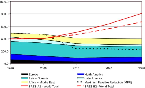
leads to significantly lower growth in emissions of the air pollutants NO_x, NMVOC and CO than was suggested by the widely used IPCC (Intergovernmental Panel on Climate Change) SRES (Special Report on Emission Scenarios) scenarios (Nakicenovic et al., 2000).

With the TM3 and STOCHEM models we performed several long-term integrations 20

(1990–2030) to assess global, hemispheric and regional changes in CH₄, CO, hy-droxyl radicals, ozone and the radiative climate forcings resulting from these two emis-sion scenarios. Both models reproduce realistically the observed trends in background ozone, CO, and CH₄concentrations from 1990 to 2002.

For the “current legislation” case, both models indicate an increase of the annual 25

average ozone levels in the Northern hemisphere by 5 ppbv, and up to 15 ppbv over the Indian sub-continent, comparing the 2020s with the 1990s. The corresponding higher ozone and methane burdens in the atmosphere increase radiative forcing by

(4)

ACPD

4, 8471–8538, 2004

Full Screen / Esc

Print Version Interactive Discussion approximately 0.2 Wm−2. Full application of today’s emissions control technologies,

however, would bring down ozone below the levels experienced in the 1990s and would reduce the current radiative forcing of ozone and methane by approximately 0.1 Wm−2. While methane reductions lead to lower ozone burdens and to less radiative forcing, further reductions of the air pollutants NO_x and NMVOC result in lower ozone, but at 5

the same time increase the lifetime of methane. Control of methane emissions appears an efficient option to reduce tropospheric ozone as well as radiative forcing.

1. Introduction

Methane (CH₄) and ozone (O₃) are both key components driving climate change and atmospheric chemistry. Methane concentrations have more than doubled since the 10

pre-industrial era, leading to a radiative forcing of about 0.5 Wm−2(Prather et al., 2001). This growth makes methane therefore, after CO₂, the second most important increas-ing greenhouse gas in the atmosphere. In large parts of the Northern Hemisphere photo-oxidation of CH₄and carbon monoxide lead to net photochemical production of O₃ (Crutzen, 1974), whereas ozone destruction prevails in NO_x deficient air in parts 15

of the tropics and the Southern Hemisphere (SH). Overall, the combined effect of in-creasing CH₄, CO, NMVOC and NO_x emissions has resulted in elevated tropospheric O₃ levels since pre-industrial times, associated with a net radiative forcing of about 0.35 Wm−2 (Ramaswamy et al., 2001).

Besides being a potent greenhouse gas, O₃ is also toxic to humans, animals and 20

plants (Buse et al., 2003; WHO, 2003). Ozone levels at a given site are influenced by several factors: (i) background concentrations of ozone and precursor gases, which are determined by large-scale processes, such as stratosphere-troposphere exchange, and global to hemispheric-scale precursor emissions; (ii) regional and local emissions; and (iii) synoptic meteorology, which can favour O₃production, e.g. during a stable high 25

pressure period in summer. Combined, these factors can lead to frequent violations of the contemporary air quality standards for ozone.

(5)

ACPD

4, 8471–8538, 2004

Full Screen / Esc

EGU Traditionally, the focus of ozone air quality control has been put on the abatement of

its local and regional precursor emissions in order to ameliorate short-term episodes of peak ozone concentrations that were considered harmful to human health and veg-etation. Recent epidemiological studies reveal damage to human health from ozone not only during such peak episodes but detect significant negative health impacts at 5

much lower concentrations, even at present northern hemispheric background levels (WHO, 2003). Based on this finding, the increasing contributions from the interconti-nental transport of ozone and ozone precursor gases (Akimoto, 2003), and increasing ozone background concentrations (Vingarzan, 2004), become of immediate concern to air quality managers throughout the world.

10

A comprehensive model intercomparison exercise involving ten global chemistry-transport models and using projections of the emissions of ozone precursor gases published in the Intergovernmental Panel on Climate Change (IPCC) Special Report on Emission Scenarios (SRES) (Nakicenovic et al., 2000) proposed near-surface ozone to increase by 2030 on average by about five ppbv in much of the Northern hemisphere 15

(Prather et al., 2003) compared to the present background levels of 30–35 ppbv. In the “worst case” (A2p) emission scenario of SRES, background ozone may grow by more than 20 ppbv up to the year 2100 relative to 2000. Obviously, such increases in background ozone would seriously degrade local air quality throughout the globe and counteract the impacts of costly local and regional emission controls.

20

However, in the last few years the threat to human health posed by ground-level ozone and particles (“air pollution”) has become a universal public concern, notably also in many cities in developing countries which face rapidly increasing car fleets (Shah et al., 1997; World-Bank, 1997) A number of national and international initia-tives have been taken to approach the problem (e.g. the Asian Clean Air Initiative of 25

the World Bank,http://www.cleanairnet.org/caiasia/). As a consequence, after the year 2000 and after publication of the SRES emission projections report, many of the major developing countries in Asia and Latin America have issued legal regulations request-ing advanced emission control techniques for mobile sources. Once fully implemented,

(6)

ACPD

4, 8471–8538, 2004

Full Screen / Esc

Print Version Interactive Discussion these regulations will significantly reduce the growth of air pollution emissions at the

regional and global scale, most notably of NO_x, NMVOC and CO, compared to earlier projections.

Climate Change policies, on the other hand, focus mostly on CO₂ emission reduc-tions, although within the Kyoto protocol (http://unfccc.int/resource/convkp.html) CH_4, 5

as well as some other greenhouse gases, are considered. Ozone, however, is not part of the Kyoto protocol. The additional global radiative forcing by ozone and methane between 2100–2000 in the aforementioned SRES A2p scenario was 0.87 Wm−2 and 0.59 Wm−2, respectively. For comparison: this adds 32% to the forcing of CO₂alone in the same time period, illustrating the potential importance of ozone and methane and 10

ozone as greenhouse gases.

There is an increased awareness (Hansen et al., 2000) that the most feasible emis-sion reduction strategies are those that take the synergies between air pollution and climate issues into account. For example Fiore et al. (2002) discuss the strong coupling between methane increases and ozone levels; methane emission reductions could 15

both reduce harmful O₃concentrations and reduce radiative forcing.

In this work we systematically focus on the interaction between CH₄and ozone pre-cursor gases emission controls and their impact on air pollution and climate forcing. Our analysis focuses on the next decades up to 2030, which is of immediate relevance for today’s policy decisions.

20

In Sect. 2 we present a set of global emission projections for the four ozone precursor gases that take into account the recent changes in air quality legislation (CLE). A sec-ond set of scenarios describes the maximum feasible emission reductions (MFR) if the full scope of today’s emission control technologies would be implemented in the next decades. Similarly scenarios are developed for anticipated changes in CH₄emissions. 25

We compare these scenarios with earlier studies and describe how they were used in the model calculations. Section 3 provides a brief description of the TM3 and STOCHEM CTM models that we used for the simulations. Section 4 compares model results with observations from the period 1990–2002. In Sect. 5, we explore the

(7)

re-ACPD

4, 8471–8538, 2004

Full Screen / Esc

EGU sulting impacts on global background ozone concentrations, methane lifetime and in

Sect. 6 we focus on radiative forcing. In Sect. 7 we discuss the results, and we present the conclusions in Sect. 8.

2. Emissions

In this work we use a set of emissions scenarios developed at the Institute for Ap-5

plied Systems Analysis (IIASA) using the global version of the Regional Air Pollution Information and Simulation (RAINS) model (Amann et al., 1999). The RAINS Current Legislation Scenario (CLE) is based on national expectations of economic growth and present emissions control legislation. The RAINS Maximum Feasible Reduction (MFR) scenario explores the scope for reduced global emissions offered by full application of 10

today’s most advanced emission control techniques. The RAINS scenarios consider agricultural, fossil fuel and biofuel related emissions from CO, NO_x, and CH₄ for the base years 1990, 1995, 2000, 2010, 2020 and 2030. A more extensive description of assumptions made, activity data and emission factors is given in the Appendix. Since RAINS concentrates on the assessment of national emissions, emissions from interna-15

tional shipping and air traffic were not included. Likewise, emissions from large scale biomass burning (deforestation, savannah, agricultural waste burning, and forest fires) and natural emissions are not included in RAINS. For atmospheric calculations these emissions were taken from other studies and added to the national emissions calcu-lated by RAINS, as described in Sect. 2.2.

20

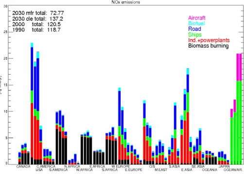
2.1. RAINS projections of anthropogenic emissions 2.1.1. Nitrogen oxides

Figure 1 gives an overview of the temporal and regional development of the RAINS CLE and MFR calculated anthropogenic NO_x emissions. Our calculations indicate

(8)

ACPD

4, 8471–8538, 2004

Full Screen / Esc

Print Version Interactive Discussion a strong decline in Europe and an approximate stabilization in North America of NO_x

emissions, due to present emission control legislation, despite the assumed underlying economic growth (by 2.3 and 1.7 % yr−1, respectively) and the corresponding increase in energy use and transport volumes. For Asia, current national expectations anticipate a growth in transport demand by a factor of 4–5. However, under the assumption of full 5

implementation of the recently decided vehicle pollution control legislation, NO_x emis-sions in Asia will not grow until 2030 by more than 35% from present days levels. Latin American NO_x emissions are expected to stabilize due to recently imposed control re-quirements in the majority of countries in this region. At the global level, this moderate increase in NO_xemissions from developing countries would be partly offset by the de-10

cline in European emissions, resulting in a global anthropogenic NO_xemissions growth of not more than 13% in the year 2030.

Despite the control measures imposed by recent legislation, full application of present best available technology could lead to significant further reductions in the global NO_x emissions, by approximately 70% in 2030 for the MFR scenario. We as-15

sume globally emission controls for vehicles and off-road sources up to the EURO-IV/EURO-V standard, for large stationary sources the application of selective catalytic reduction and for small stationary boilers the use of low-NO_x burners. Obviously, the scope for further emission reductions strongly depends on the stringency of the al-ready implemented measures and thus differs greatly between countries. While there 20

will be a limited potential for further reductions in Europe and North America, there re-mains significant scope in many developing countries. Sectoral emissions for the two scenarios as well as details by country/region are available from Cofala (2004b). 2.1.2. Carbon monoxide

In Fig. 2 we give an overview of the RAINS CO emissions. Biomass burning (not 25

included in Fig. 2) is a very important source for CO, as further discussed in Sect. 2.2. Our analysis suggests, despite increasing economic activities, a global reduction of anthropogenic CO emissions in the coming three decades in both the CLE (−15%) and

(9)

ACPD

4, 8471–8538, 2004

Full Screen / Esc

EGU MFR (−53%) scenario. The highest decline (−55%) occurs in Latin America, which is

mainly due to a switch from fuel wood to other energy carriers in the residential sector. The only region with increasing emissions is Africa (+10%). The decoupling between economic growth and emissions is caused by the declining combustion of coal and fuel wood in households in small stoves and the penetration of three-way catalysts that 5

reduce CO emissions from vehicles by typically between 80% and 90%.

The maximum technically feasible reduction (MFR) scenario assumes full EURO-IV/EURO-V emission control standards for mobile sources, as well as good house-keeping measures on stationary combustion sources. However, this scenario does not consider possible reductions in energy demand (e.g. through energy efficiency mea-10

sures) nor the potential offered by substitution of solid fuels by less polluting forms of energy. Based on these assumptions, the analysis suggests for 2030 a maximum re-duction of CO emissions of 53% compared to the year 2000. Similarly to NO_x, sectoral and country details can be found in Cofala (2004b).

2.1.3. Methane 15

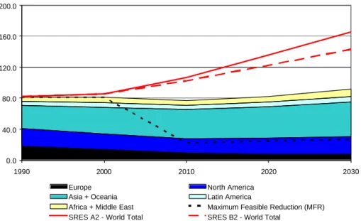
In Fig. 3 we give an overview of the RAINS CH₄emissions. Our analysis suggests for the CLE case a continued increase of global anthropogenic CH₄emissions, leading to 35% higher emissions in 2030 than in 2000. Overall, emissions from all sectors are expected to grow due to increased economic activities and in the absence of wide-spread emission control measures. In contrast to the emissions of non-greenhouse 20

gases NO_x and CO, the calculated growth in CH₄ emissions is well within the range spanned by the SRES greenhouse gas scenarios.

A wide range of technical measures is presently available to reduce methane emis-sions. Such measures include the treatment of manure to generate biogas, different feedstock to prevent methane losses from enteric fermentation, prevention of waste dis-25

posal, controlling waste disposal sites, reduction in distribution losses of natural gas, gas recovery in coal mines as well as during oil and gas extraction, alternative rice strains, etc. (EPA, 1999; Hendriks et al., 1998). If all these “maximum technically

(10)

fea-ACPD

4, 8471–8538, 2004

Full Screen / Esc

Print Version Interactive Discussion sible reductions” were applied to the full extent, global CH₄ emissions would stabilize

up to 2030. Country and sectoral details are to be found in Mechler (2003). 2.2. Other emissions

For use in the TM3 and the STOCHEM CTM models, gridded emission data need to be provided. Thus, we allocated the national estimates for each sector according to 5

the gridded sectoral distribution of emissions of the EDGAR3.2 global emission inven-tory (Olivier et al., 1999). We further linearly interpolated the data between the base years. Furthermore the previously discussed IIASA emission data had to be supple-mented with estimates for international sea-traffic, aircraft emissions, biomass burning and natural emissions. The resulting emissions are provided in Figs. 4, 5, and 6, giving 10

a regional and a lumped sectoral break-down of the gridded anthropogenic NO_x, CO and CH₄emissions for the years 1990, 2000 and 2030 (the latter both CLE and MFR) using the IMAGE2.2 (http://arch.rivm.nl/image/) regional classification.

For sea traffic, we used the 1995 estimates provided in the EDGAR3.2 database and augmented them with a moderate growth rate of 1.5% yr−1over the time horizon of our 15

study, without distinguishing between the “current legislation” and “maximum feasible reduction” cases. The resulting emissions are consistent with the lower case projection developed by MARTINEK (2000). As we show in Fig. 4 sea-traffic already plays an important role for global NOx emissions, and may in future be larger than the emissions from any single region. Emissions from aircrafts were only considered for NOx and 20

were taken from the IPCC Special Report on Aviation and the Global Atmosphere (Isaksen et al., 1999). We calculated a polynomial fit to the global emission numbers of 2.6 Tg NO₂yr−1in the year 2000 and 5.7 Tg NO₂yr−1 in 2030 and applied them for both scenarios.

For emissions from biomass burning we used the EDGAR3.2 1990 and 1995 25

amounts and spatial distributions for savannah burning, deforestation fires, agricul-tural waste burning and temperate forest fires. To account for more recent insights regarding emission factors and activity data (Arellano Jr. et al., 2004; Bergamaschi

(11)

ACPD

4, 8471–8538, 2004

Full Screen / Esc

EGU et al., 2000b; van der Werf et al., 2003) we doubled these amounts leading in the

year 2000 to global biomass burning emissions of 27 Tg NO₂ yr−1, 575 Tg CO yr−1, 65 Tg CH₄ yr−1, and 80 Tg NMVOC yr−1. These numbers are at the high side of the estimates given by e.g. Andreae and Merlot (2001), but it should be noted that exact amounts of biomass burning are not well established and subject to large inter-5

annual fluctuations. The biomass burning source is most critical for the CO budget (http://www.sdearthtimes.com/et0701/et0701s12.html; (Wild et al., 2001). On the other hand, in IPCC TAR Prather et al. (2001) an amount of 700 Tg CO yr−1 was recom-mended, 25 % higher than in this study. In accordance with the assumptions made in the IIASA MESSAGE implementation of the B2 scenario the emissions from defor-10

estation are gradually declining to zero in the year 2020 (for both CLE and MFR). In contrast, the by far larger emissions from savannahs and high latitude fires remained almost constant.

In S. America, and large parts of Africa, NO_x emissions are dominated by biomass burning, whereas industrial and traffic related emissions dominate in the US, Europe 15

and Asia (Fig. 4).

Figure 5 shows the important, but very uncertain role of biomass burning related CO emissions in Africa, Oceania, and South America. It should be noted that the use of EDGAR3.2 emissions results in quite high CO emissions at Northern Latitudes. Biofuel is an important source for CO in Asia, whereas industrial and traffic emissions dominate 20

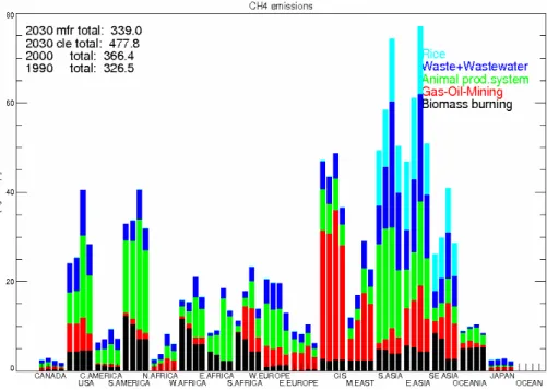
in Europe, USA and Japan. Figure 6 displays the variable importance of different CH₄ sources in the world regions: Rice production and waste dominate in Asia, gas-oil and mining in Russia and the Middle East, whereas waste, animal production systems dominate methane emissions in the US, S. America, and Europe.

For natural emissions we consider NO_x emissions from soils and lightning (ca. 38 25

Tg NO₂ yr−1, CO emissions from soils and oceans (ca. 150 Tg CO yr−1), and CH₄ emissions from wetlands, termites, permafrost melting, volcanoes and oceans (ca. 240 Tg CH₄yr−1). The natural NMVOC emissions are predominantly isoprene emissions from vegetation (507 Tg C yr−1). For both scenarios, we kept these emissions constant

(12)

ACPD

4, 8471–8538, 2004

Full Screen / Esc

Print Version Interactive Discussion over time. Since some of the emissions are hard-wired into the model code, they differ

slightly among the models and years (see Sect. 3).

Finally, in this work no separate assessment has been made for NMVOC emissions. We assumed that the anthropogenic NMVOC emissions trends closely follow the de-velopment of CO emissions. This assumption is justified for mobile sources since 5

three-way catalysts applied to mobile sources simultaneously reduce CO and NMVOC emissions with similar efficiency. Global emissions amount to ca. 250 Tg yr−1 in the year 2000 (including biomass burning), and 293 and 226 Tg yr−1 in the year 2030 for the CLE and MFR scenario, respectively.

3. The atmospheric chemistry transport models

10

3.1. The TM3 model

The Eulerian global chemistry-transport model TM3 (Dentener et al. (2003a), and ref-erences therein) has been used in this study at a spatial resolution of 10◦ longitude and 7.5◦latitude with 19 vertical layers, with approximately 14 layer in the troposphere. In this study the model used annually repeated 1990 meteorological fields from the 15

ECMWF ERA15 re-analysis (Gibson et al., 1997). These fields include global distri-butions for horizontal wind, surface pressure, temperature, humidity, cloud liquid water content, cloud ice water content, cloud cover, large-scale and convective precipitation provided in 3–6 h time steps. In a pre-processing chain these fields were used to cal-culate turbulent diffusion coefficients according to (Louis, 1979) and convective mass 20

fluxes using a modified Tiedke scheme (Tiedke, 1989) that accounts for shallow, mid-level and deep convection. Tracer advection is described with the slopes scheme of Russell and Lerner (1981). The chemical scheme is a modified CBM4 mechanism that describes CH₄-CO-NMVOC-NO_x-SO_xchemistry (Houweling et al., 1998) and consid-ers 47 species, and 91 reactions. The chemical equations are solved with and Euler 25

(13)

ACPD

4, 8471–8538, 2004

Full Screen / Esc

EGU of soluble trace gases and aerosol by wet deposition is based on the work of Guelle et

al. (1998) and Jeuken et al. (2001) and accounts for wet removal in and below cloud in stratiform and convective rain. Dry deposition follows a resistance approach and is de-scribed by Ganzeveld et al. (1998). Stratospheric boundary conditions for ozone and HNO₃ were relaxed to satellite observations above 50 hPa as described in Lelieveld 5

and Dentener (2000). CH₄ stratospheric loss rates were prescribed at a fixed rate of 40 Tg CH₄ yr−1, and the CH₄ soil sink kept constant at 30 Tg CH₄ yr−1. We showed before that the model realistically simulates Radon-222 (Dentener et al., 1999), tro-pospheric ozone (Houweling et al., 1998; Lelieveld and Dentener, 2000; Peters et al., 2001) and methane (Dentener et al., 2003b; Houweling et al., 2000a). A recent study 10

was devoted to study OH trends (Dentener et al., 2003a) and is in particular relevant for this study, since that model set-up was used almost unchanged in the present study. 3.2. The STOCHEM model

STOCHEM is Lagrangian tropospheric chemistry-transport model, originally described by Collins et al. (1997). In this study the atmosphere is divided in 50000 air parcels 15

that are mapped after each advective time-step to a 5 by 5◦resolution grid with 9 verti-cal layers of 100 hPa thickness. Input meteorology is provided by the atmosphere-only climate model HadAM3 (Pope et al., 2000) at a standard resolution of 3.75 longitude and 2.5 latitude with 19 vertical levels extending to 10 hPa. The HadAM3 time-step is 30 min, with meteorological fields passed to STOCHEM every 3 h. HadAM3 was 20

forced with monthly mean sea surface temperature (SST) climatology for the period 1978–1996 (Taylor et al., 2000); i.e. they have a seasonal structure, but are annu-ally invariant. Land surface temperatures are calculated by the GCM and show some inter-annual variability. Consequently also the wind fields display some inter-annual variability. Turbulent mixing in the boundary layer is achieved by randomly re-assigning 25

the vertical co-ordinates of air parcels over the depth of the planetary boundary layer height, which is provided by the HadAM3 model. Convective mixing uses updraft and detrainment fluxes from HadAM3 as described by Collins (2002). Air parcel advection

(14)

ACPD

4, 8471–8538, 2004

Full Screen / Esc

Print Version Interactive Discussion is performed using a fourth order Runge-Kutta method; at each 1 h advection time step

the winds are linearly interpolated to the parcel’s location in the horizontal and using cubic interpolation in the vertical. The chemical scheme, as described by Collins et al. (1999) includes 70 species that take part in 174 photochemical gas and aqueous phase reactions. The chemical scheme uses a Backward Euler solver (Hertel et al., 5

1993) using a time step of 5 min. Wet deposition operates on all soluble species, with scavenging coefficients taken from (Penner et al., 1994). The scheme is described in more detail in Stevenson et al. (2003). Dry deposition follows a resistance approach as described by Sanderson et al. (2003) including explicit description of the CH₄ soil sink. Ozone and NO_y upper boundary conditions are imposed by prescribing fluxes 10

into the top layer of the model at 100 hPa. For this vertical winds derived from HadAM3 at 100 hPa were used together with the ozone climatology of Li and Shine (1995). NO_y influxes were fixed to those of O₃ by assuming a fixed mass ratio of N:O₃ of 1:1000. CH₄stratospheric loss rates were prescribed following Prather et al. (2001).

As described above STOCHEM and TM3 represent different types of models using 15

very different parameterizations and meteorological input datasets. In the next sec-tion we will document some salient features of model performance to show that the combination of the models set-up and emissions is realistically describing global scale measurements of ozone, methane and carbon monoxide.

4. Simulations

20

4.1. Description of simulations

In order to simulate the future developments of ozone and methane we performed 6 simulations summarized in Table 1. The simulations were integrated from 1990–2030, using a spin-up of 13 months for STOCHEM and 24 months for TM3, respectively. Both TM3 and STOCHEM used CLE and MFR scenarios, the sensitivity studies MFR-CH₄ 25

(15)

ACPD

4, 8471–8538, 2004

Full Screen / Esc

EGU 4.2. Comparison with measurements

Although in previous applications of the TM3 and STOCHEM models extensive com-parison to measurements has been made, in this work we use a completely new set of emissions. In this section we show a selection of measurements to demonstrate that the 1990–2003 part of our simulations are consistent with current observations 5

and can be safely used to extrapolate to future conditions. For analysis, we divide the globe into four regions, stretching from 90◦S–45◦S, 45◦S-Equator, Equator-45◦N, and 45◦N–90◦N.

4.3. Surface ozone

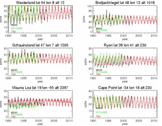
In Fig. 7 we present surface ozone calculated by TM3 and STOCHEM at 6 stations, 10

mostly located in the Northern Hemisphere. Data were retrieved from the world data center for surface ozone (WDSO) (http://gaw.kishou.go.jp/wdcgg.html), with the addi-tional data for Cape Point kindly provided by Drs. E. Brunke. The data sets appear quite heterogeneous, and those that cover the entire 1990s are scarce. We selected back-ground stations that our relatively coarse models should be able to represent. Thus 15

stations that may be strongly influenced by local emissions were not considered. No selection of data was applied. Generally the TM3 and STOCHEM models represent relatively well the set of background stations given in Fig. 7. Of course there are also some discrepancies: especially at continental stations the difference of models with measurements can be of the order of 10–15 ppbv; this can be explained from uncer-20

tainties in emissions, chemistry and especially the coarse model resolution chosen for the scenario simulations. No strong trends are visible in either the models or the mea-surements over the time period considered. For comparison we show for TM3 both the ozone concentrations calculated with CLE and MFR out to 2010. The difference of the ozone signal in summer between these two scenarios is about 10 ppbv by the year 25

(16)

ACPD

4, 8471–8538, 2004

Full Screen / Esc

Print Version Interactive Discussion 4.3.1. Tropospheric ozone in the middle and upper troposphere

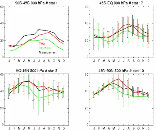
In order to evaluate model performance in the middle and upper troposphere, we use the ozone climatology compiled by Logan (1999) based on an analysis of ozone sound-ings obtained predominantly during the period 1985–1995. About 55 stations were se-lected; 3 stations were located in the region 90◦S–45◦S, 20 in the region 45◦S-Equator, 5

19 stations from the Equator-45◦N, and 13 stations from 45◦N to 90◦N. Monthly aver-age model results for the period 1990–2000 were interpolated to the geographical sta-tion locasta-tion and pressures. In Figs. 8a and 8b we display results obtained at 800 hPa, and 400 hPa, respectively. The error bars represent the standard deviations of the set of individual soundings contributing to the regional average, rather than the inter-annual 10

variability within the individual measurements contributing to the monthly averages. We present our results in this way, since we compare model results obtained using mete-orology for a specific year, 1990 in the case of TM3, or a decade of climate model calculated years for STOCHEM, and compare them to measurements representative for other years.

15

At 800 hPa in the SH both TM3 and STOCHEM slightly underestimate ozone by 5–10 ppbv. In the other regions both TM3 and STOCHEM reproduce the seasonal cy-cle of O₃ well within the standard deviation of the measurements. At 400 hPa in the middle/upper troposphere TM3 generally realistically reproduces the measurements, whereas STOCHEM underpredicts O₃ by 10–15 ppbv. However, especially in the 20

45◦S–90◦S region in summer TM3 also underestimates ozone. The problem seems related to the amount of stratosphere-troposphere exchange, and the exact height of the tropopause, since the observed concentrations and variability indicated the influ-ence of stratospheric air, whereas TM3 rather calculates tropospheric ozone values and variability. Nevertheless, all in all both models give a realistic picture of ozone 25

(17)

ACPD

4, 8471–8538, 2004

Full Screen / Esc

EGU 4.3.2. Carbon monoxide

Figure 9 displays the annual averaged carbon monoxide measurements and model results for the four world regions. We use the monthly mean NOAA CMDL measure-ments (http://www.cmdl.noaa.gov/), as reported by, e.g. Dlugokencky et al. (1996) and Dlugokencky et al. (2003). We used only those stations with a complete dataset for the 5

period 1994–2002, and averaged them in 4 regions and annual averages. The TM3 and STOCHEM model results interpolated to the geographical location and altitude of the stations were averaged in the same way. In the SH TM3 overestimates CO by about 5–15 ppbv. In the Northern Hemisphere TM3 calculated CO levels correspond accu-rately to the measurements, whereas the STOCHEM CO levels were underestimated 10

by up to 15–30% (10–20 ppbv) in the NH (Northern Hemisphere), and up to 50 ppbv in the high latitude zones.

We also present the standard deviations of the annual model concentrations and measurements, representing the spatial variability among stations in a particular year. Both in the NH and SH the measured and modelled error bars are similar, meaning 15

that the gradients of CO close to the continents and on the ocean are well captured. In the Northern Hemisphere in 1998 measurements on average were elevated by 10– 20 ppbv compared to other years. This increase is related to large scale biomass burn-ing in Indonesia (Duncan et al., 2003) followburn-ing the intensive ENSO (El Ni ˜no Southern Oscillation) of 1997/1998, and large forest fires in Canada and Siberia (Simmonds 20

et al., 2004; Wotawa et al., 2001; Yurganov et al., 2004). This signal is not seen in STOCHEM and TM3 since we did not account for inter-annual variations in biomass burning. As indicated in Sect. 2.4 the uncertainties in the biomass burning emissions are large. Since the inter-annual variability in the CO measurements is high, it is at this moment not possible to confirm how realistic the decreasing model trend in the period 25

1995–2002 is realistic. The decreasing model trend, however, seems to be found by measurements at e.g. Mace Head, that indicate a decreasing trend of 1.13 ppbv/yr in baseline air masses (Simmonds et al., 2004). Models and measurements agree on the

(18)

ACPD

4, 8471–8538, 2004

Full Screen / Esc

Print Version Interactive Discussion absence of a CO trend in the SH.

4.3.3. Methane

We present annual average methane concentrations for the four world regions in Fig. 10. As for CO, CH₄measurements were obtained form the NOAA CMDL network; since more measurements were available we could use the full record for 1990-2002. 5

Due to inaccuracies in the initialization, which was done differently in both models, TM3 CH₄ is about 30–40 ppbv lower than the measurements, whereas STOCHEM is about 30 ppbv higher. We estimate that the influence of this inaccuracy of the initial CH₄concentrations on global OH is of the order of 1% (using the feedback factor of

d ln[OH]/d ln[CH₄]=−0.32, Prather et al., 2001). This is small in comparison to over-10

all uncertainties of global OH. In the 1990s the measured methane growth rates were highly variable, ranging from 0 to 15 ppbv yr−1 (Butler et al., 2004; Dentener et al., 2003b; Dlugokencky et al., 2003; Prather et al., 2001) with an average trend of 8 ppbv yr−1.

Although this variability of growth rates is not represented by our models, the average 15

methane increases in the period 1990–2002 are on average well represented, although TM3 has a somewhat low trend at the beginning of the 1990s. After the year 1998 both TM3 and STOCHEM predict a too high trend. Interestingly, after the year 2000 the use of the MFR emission scenario seems to agree better with the measured trend than CLE, although shifted by two or three years. We discuss the significance of this in 20

(19)

ACPD

4, 8471–8538, 2004

Full Screen / Esc

EGU 5. Scenario calculations

5.1. Budgets of CH₄, CO, OH and O₃ 5.1.1. The budgets for 2000

The budgets for TM3 and STOCHEM for the four regions in the year 2000 are pre-sented in Table 2. As was also visible in the surface concentrations (Fig. 10), the 5

TM3 CH₄ budgets are somewhat lower than those of STOCHEM, mainly resulting from the initialization. Both models produce similar levels and trends in CO burdens for the 1990s, except in the 45◦N–90◦N compartment, were we showed before that STOCHEM underestimated CO by ca. 15–30%, possibly related to larger OH burdens. The global O₃ burdens calculated by TM3 are 15% higher than those of STOCHEM; 10

the difference mainly occurs in the tropics and SH. There are many processes that can explain the model differences, but one important one is the difference in our pa-rameterizations of convection, strongly influencing the lifetime of ozone in the tropics. The STOCHEM results clearly show inter-annual variability, mainly resulting from vari-ability in the stratosphere-troposphere exchange processes, which are partly driven by 15

HadAM3 vertical winds at 100 hPa. As explained before, in HadAM3 only SSTs were kept constant, whereas land surface temperatures were not constrained, leading to inter-annual variability of meteorology. In contrast TM3 always used the meteorology representative for the year 1990. There is disagreement between the models on global OH burdens. Globally, STOCHEM calculates about 25% more OH than TM3, because 20

of differences in water vapor, photo-dissociation rates, and OH production in the free troposphere. Despite the differences in OH column amounts, global CH₄lifetimes are similar in the year 2000. This can be explained by the fact that the destruction of CH₄is mostly sensitive to the high OH concentrations in the humid and warm tropical regions, and is not particularly sensitive to middle and upper tropospheric and extra-tropical OH 25

(20)

ACPD

4, 8471–8538, 2004

Full Screen / Esc

Print Version Interactive Discussion 5.1.2. Budget trends

In Figs. 11a–11e we present the calculated global lifetime with regard to oxidation by OH of CH₄, and the atmospheric burdens of CH₄, CO, O₃ and OH integrated up to 100 hPa for simulations the CLE and MFR scenarios for TM3 and STOCHEM, and MFR-CH₄ and MFR-pol for TM3. 100 hPa corresponds to the tropical tropopause, 5

and hence the burdens contain some stratospheric air at middle and high latitudes. Note that for the period 1990–2000 the simulated results for all scenarios are identical. To visually highlight the model trends, rather than model differences, we normalized in Fig. 11 the STOCHEM results to match the TM3 results of the year 2000. In the following discussion we will use these normalized numbers.

10

The global CH₄burdens for the CLE case increase from 4300 Tg in the year 2000 to 5300 Tg in 2030 for TM3, and to 5000 Tg for STOCHEM. For the MFR case, both mod-els calculate methane burdens stabilizing at 4300 Tg. Considering MFR-CH₄ where only methane emissions are reduced but NO_x, CO and NMVOC emissions develop according to CLE, the global methane burden would decrease by 1000 Tg below the 15

CLE level calculated for 2030. Alternatively, assuming maximum feasible reductions for NO_x, NMVOC and CO but leaving CH₄at the CLE development (simulation MFR-pol) would in 2030 increase the global methane burden by 400 Tg above the CLE case. This increased CH₄ burden resulting from the same CH₄ emissions is caused by the prolonged lifetime of methane due to lower availability of OH radicals that serve as CH₄ 20

sinks. OH is reduced as a consequence of the lower NO_x, CO and NMVOC emissions. Despite the differences in methane burden in STOCHEM and TM3 (Table 2), and pos-sible consequences for OH, the temporal changes of methane lifetime and burden are very similar in TM3 and STOCHEM. The increases of methane burdens correspond to roughly 1750 ppbv in the year 2000 and 2200 ppbv (TM3) and 2090 ppbv (STOCHEM) 25

for CLE.

Both models suggest for the CLE case stable global CO burdens at approximately ∼380 Tg (CLE), and a gradual decrease to 320 Tg CO in 2030 for the MFR case.

(21)

ACPD

4, 8471–8538, 2004

Full Screen / Esc

EGU Despite model differences in the year 2000, the global O₃ burdens from TM3 and

STOCHEM show very similar increases from 450 Tg in 1990 to 470–485 Tg in 2030 in the current legislation (CLE) case, and decreases to 430 Tg for the MFR case.

Despite the large discrepancies in the 2000 OH burdens, both models agree on sta-ble OH burdens for both the CLE and MFR scenarios. It is interesting to note here that 5

the MFR-CH₄and MFR-NO_x simulations, calculated with TM3, affect the OH burdens more strongly than the ‘balanced’ CLE and MFR simulations.

The corresponding calculated CH₄lifetime trends (Fig. 11a) indicate a rather stable CH₄ lifetime in the next decades for both the CLE and MFR scenario. However, the TM3 calculations show that preferential air pollution controls MFR-pol tend to lengthen 10

the methane lifetime, whereas the MFR-CH₄ case has an opposite effect. The latter effect is a manifestation of the methane self-feedback (Isaksen and Hov, 1987) where tropospheric OH decreases with increasing methane, and visa versa.

5.2. Surface ozone in the 1990s and 2020s

In this section we explore the regional changes in surface ozone for the various sce-15

narios, which are of importance for air pollution issues. We focus on annual average ozone, as well as Northern Hemisphere summer concentrations.

In Figs. 12a–12c we present the annual average computed ozone concentrations at the surface averaged for the 1990s and 2020s, while Figs. 13a–13c focuses on the dif-ference between the 2020s and 1990s. For the 1990s, with few exceptions, the models 20

show broad agreement on the regional patterns of surface ozone concentrations, al-though the STOCHEM model consistently calculates 5 to 10 ppbv higher ozone levels over the continents and lower values over the oceans. Average volume mixing ra-tios range from 30 to 60 ppbv. The high concentrations calculated over the Himalayas are due to high altitude of this region, and strong mixing with stratospheric air. The 25

biomass burning signal in tropical Africa is much stronger present in STOCHEM than in TM3, probably due to differences in the mixing schemes of the two models, or in the implementation of biomass burning emissions in our models.

(22)

ACPD

4, 8471–8538, 2004

Full Screen / Esc

Print Version Interactive Discussion In the 2020s under the CLE scenario TM3 and STOCHEM ozone background

concentrations reach annual average levels of 50–60 ppbv in large parts of the NH (Fig. 12b) with highest levels found over the Mediterranean, the Arabian and Indian Peninsulas, and China. Assuming MFR emission reductions, annual average ozone levels are in the range of 35–45 ppbv in the 30◦N–45◦N latitude band, and below 5

35 ppbv at latitudes larger than 45◦N (Fig. 12c). In the SH O₃remains at 10–20 ppbv. A perhaps more robust calculation is the difference of calculated ozone concentra-tions under the various scenario assumpconcentra-tions during the 2020–2030 period and the baseline period 1990–2000. The results of TM3 and STOCHEM (Fig. 13a) are quite consistent, showing maximum increases of ozone levels between 8–12 ppbv in India, 10

Pakistan and Bangladesh, China and South East Asia. Over the North Pacific and Atlantic Ocean ozone increases by 4–6 ppbv, related to increases in ship emissions, whereas over the other world regions ozone remains largely unchanged. Interestingly, despite emissions reductions in North America and Europe in the CLE scenario (Fig. 1 and Fig. 4), the computed ozone levels in the 2020s do not decrease, but even some-15

what increase, clearly illustrating the global nature of ozone control strategies, as well as non-linear NO_x, NMVOC chemistry.

For MFR (Fig. 13b), TM3 calculates ozone decreases of about 5 ppbv over much of the NH, and up to 10 ppbv in the USA, Middle East and South East Asia, comparing the 2020s with the 1990s. A slight increase in ozone is predicted over North and Central 20

Europe, an ozone-NO_x titration effect, which may be dependent on the coarse model resolution. The STOCHEM model (Fig. 13b) displays a stronger response of surface ozone to emission reductions, with reduced concentrations in large parts of Eastern Europe and Russia. The difference of MFR-pol in the 2020s with CLE in the 1990s (Fig. 13c) shows the effect of NO_x, CO and NMVOC reductions (following the MFR 25

scenario) whilst CH₄ emissions follow the CLE scenario. It shows that, as expected, the largest effect on ozone of emission reductions stems from air pollutant controls.

We also isolate in Fig. 13c (lower panel) the effect of CH₄abatement, by comparing MFR-CH₄ with CLE in the 2020s, showing a uniform ozone reduction by 1–2 ppbv

(23)

ACPD

4, 8471–8538, 2004

Full Screen / Esc

EGU throughout most of the NH and SH.

It is interesting to observe that the effect of emission reductions is quite linear, e.g. the results of simulation MFR can be largely explained by the combination of MFR-CH₄and MFR-pol. Thus about one third of the O₃reductions associated with the MFR scenario can be obtained by CH₄emission reductions!

5

While recent epidemiological studies have found robust evidence for health damage from ozone down to annual mean concentrations of 30–40 ppb, vegetation damage is mostly related to ozone exposure during the vegetation period, typically on days with ozone exceeding 40–50 ppbv. Focusing on the growing season of the Northern Hemi-sphere (June–August), Figs. 14a–14c reveal for the emissions of 1990 for large parts of 10

Southern Europe, the Middle East and Asia ozone mixing ratios above 50 ppbv. In the 2030 CLE simulation, this high-ozone region is strongly expanded, especially in Asia. However, considering the MFR scenario for 2030 during the vegetation growth period, ozone would fall below 50 ppbv in most parts of the world. In the SH during these winter months ozone remains relatively constant at levels between 10 and 30 ppbv.

15

6. Radiative forcing

The traditional air pollutants NO_x, CO, and NMVOC as well as the greenhouse gas methane do not only contribute to tropospheric ozone but also have direct (in the case of methane) and indirect (via ozone formation) impacts on radiative forcing. To explore these interactions, we calculated the radiative forcing of the four emission scenarios, 20

following the method described in Stevenson et al. (1998), using the radiative transfer model of Edwards and Slingo (1996).

These forcings account for stratospheric adjustment, assuming the fixed dynamical heating approximation, which reduces instantaneous forcings by ∼22%.

In the CLE scenario (Fig. 15a), ozone forcing maximizes in the subtropics, and over 25

bright high albedo surfaces. Peak values of 0.3 Wm−2 are found over India and the Arabian Peninsula, coinciding with elevated surface concentrations. In contrast, the

(24)

ACPD

4, 8471–8538, 2004

Full Screen / Esc

Print Version Interactive Discussion radiative forcings associated with MFR are similar in magnitude (0 to −0.2 Wm−2) and

distribution, but opposite in sign (Fig. 15b). The global and yearly average forcing of O₃ranges between 0.075 and −0.072 Wm−2for CLE and MFR, respectively (Table 3). Radiative forcing calculated for the ozone fields of the STOCHEM model is only 55% of the forcing computed for the TM3 ozone results (0.041 Wm−2for the STOCHEM CLE 5

case instead of 0.075 Wm−2). The difference can be explained partly by the fact that TM3 is somewhat more efficiently producing free tropospheric O₃than STOCHEM. We also note that STOCHEM results display some inter-annual variability in tropopause height, which cannot be completely masked out when comparing the decadal forc-ings calculated for the 1990s and the 2020s, and which influence significantly the 10

STOCHEM results. In this respect, TM3 results reflect more accurately the changes arising solely from the emissions changes, as these model runs include no climate variability.

Methane radiative forcing was calculated using the equation presented in Chapter 6 of the IPCC Third Assessment Report (Ramaswamy et al., 2001) Again we compare 15

the forcings for the 2020s relative to those in the 1990s. The CH₄ forcings for TM3 results are between 0.14 Wm−2for the CLE case and 0.01 Wm−2for MFR, and between 0.10 and −0.01 Wm−2 for the STOCHEM results. The lower STOCHEM forcings are caused by somewhat higher STOCHEM OH trends and correspondingly lower CH₄ burdens.

20

As discussed above, in the CLE scenario anthropogenic CH₄ emissions increase from 340 Tg CH₄ yr−1 in the year 2000 to 450 Tg CH₄ yr−1 in 2030. A similar emis-sion increase is given in IPCC TAR for the B2 emisemis-sion scenario. The corresponding increase in radiative forcing of 0.11 Wm−2 by the year 2030 relative to the year 2000 (0.60 Wm−2in 2030, and 0.49 Wm−2in 2000, relative to pre-industrial levels) compares 25

well with our calculations.

Compared to the current legislation (CLE) situation in the 2020s and based on TM3 calculations, maximum reduction of all four emissions (MFR) would reduce the addi-tional radiative forcing of ozone by 0.148 Wm−2 and of methane by 0.163 Wm−2, i.e.

(25)

ACPD

4, 8471–8538, 2004

Full Screen / Esc

EGU in total by 0.311 Wm−2. Just controlling methane (MFR-CH₄) would reduce the direct

forcing from methane by 0.206 Wm−2 and through the associated reductions in tro-pospheric ozone by an additional 0.046 Wm−2. Conversely, if the air pollutants were reduced but methane remained at current legislation level, the reduced forcing from the ozone reduction (−0.105 Wm−2) would be counteracted by the increased lifetime of 5

methane (forcing from methane would increase by 0.054 Wm−2), so that overall forcing would only decline by 0.051 Wm−2.

7. Discussion

7.1. Emissions

We have compiled global projections of the ozone precursor emissions based on 10

present national expectations on economic development and penetration of present emission control legislation. While the compiled growth rates in economic develop-ment (in particular for transport demand) are largely consistent with the assumptions of other global assessments, this study took into account new national legislation on mobile sources that has been adopted after the year 2000 in many developing coun-15

tries in Asia and Latin America.

For NO_x, resulting emission estimates for the year 2000 for most industrialized coun-tries do not differ by more than 5–10 % from national inventories, although there are somewhat larger differences to inventories for some developing countries published by different sources, e.g. the EDGAR3.2 emissions reference database (Olivier and 20

Berdowski, 2001). Our estimates are also consistent with the SRES estimates for the year 2000 which were 6 % higher than our assessment. However, global NO_x emis-sions are calculated to increase until 2030 by only 13% in the CLE scenario. This estimated increase is significantly lower than projections from earlier studies, including the global emission scenarios published in the IPCC SRES report (Nakicenovic et al., 25

(26)

ACPD

4, 8471–8538, 2004

Full Screen / Esc

Print Version Interactive Discussion to increase between 65 (SRES-B2) and 90% (SRES-A2). With comparable rates of

growth in the vehicle stock, the difference can be explained by the fact that the SRES scenarios did not include recently introduced air pollution control legislation in develop-ing countries. This refers first of all to legislation on mobile sources (catalytic convert-ers, engine modifications), which became mandatory in many countries in Asia, Latin 5

America, Eastern Europe and Russia. Further, the SRES simulations for the OECD countries include air pollution control measures as in force in mid-1990’s, without as-suming further changes. In our scenarios we included recently decided stricter legisla-tion in Europe (e.g. EURO IV/V standards on cars and trucks, Large Combuslegisla-tion Plant Directive, IPPC Directive for industrial sources), as well as current reduction plans in 10

North America. Without inclusion of those control measures (both in the OECD and in the developing countries) the 2030 emissions would have been 50 % higher than 2000 emissions. Approximately half of this difference results from implementation of controls in the developing world and reforming economies, and the balance is due to phasing-in more strphasing-ingent measures phasing-in the OECD countries. The remaphasing-inphasing-ing difference to the 15

marker B2 scenario (MESSAGE) can be explained by different assumptions about ac-tivity levels.

For CO, the RAINS emission estimate of the total world anthropogenic emissions (without biomass burning) are 9% lower than those of EDGAR3.2, which is mainly due to lower RAINS emissions in Europe (different assumptions on the effect of catalytic 20

converters on the emissions of mobile sources), and Asia and Russia (lower emission factors from coal and wood burning in small stoves). Also on a regional (e.g. Eu-rope, Africa) level the RAINS emissions in the year 2000 are consistent with other esti-mates (e.g. EDGAR3.2 and SRES). We predict that emission controls for vehicles and a switch from coal and fuel-wood to cleaner fuels in the residential sector decrease CO 25

emissions in most world regions, so that global CO emissions decrease by 16% from the year 2000 to 2030. Without these presently decided pollution control measures for vehicles, global CO emissions would grow in our calculations by approximately 45% up to 2030, which is close to the lower range (e.g. B1) in the SRES scenarios.

(27)

ACPD

4, 8471–8538, 2004

Full Screen / Esc

EGU Methane emissions, assuming implementation of present emission control

technol-ogy, are computed to increase by 35% up to 2030, in agreement with the range of emissions spanned by the SRES scenarios. Differences between our present day CH₄ emission estimates and country data reported to UNFCCC (http://unfccc.int) are typi-cally in the range of 10% to 30%. Note, however, that for many countries the UNFCCC 5

estimates are missing, inaccurate or incomplete, making a direct comparison difficult. There is some uncertainty about the actual implementation of new legislation in de-veloping countries, especially in the near future. However, given the pressure from the strong public concern on local air quality in many developing countries and the demonstrated progress in economical and institutional development, it does not seem 10

unreasonable to assume wide-spread compliance with the new regulations by the year 2030.

In our MFR scenario we explored the scope for reduced global emissions offered by full application of today’s most advanced emission control techniques. Although rather costly, global NO_x emissions could be reduced in 2030 by 67% compared to the year 15

2000. Using available technology anthropogenic CO emissions (excluding biomass burning) can be reduced by 53% in 2030, and methane emissions by 5% given the anticipated levels of economic activities. Obviously, some of these technical measures are costly, and full application of these measures might have repercussions on eco-nomic development. However, in our analysis we focus on the theoretical potential to 20

reduce air pollution and global warming that is offered by today’s technological means. At the same time we ignored in our analysis non-technical structural measures that modify energy demand or influence human behavior. Other studies have shown that such measures, if successfully implemented, could lead to significant emission reduc-tions, often at rather low costs (Van Vuuren et al., 2005). Therefore, we consider our 25

MFR scenario as an option for a cleaner atmosphere and a reduced contribution to the greenhouse effect.

All in all, the range of CH₄emissions increases under CLE and MFR is quite consis-tent with the IPCC SRES scenarios. Interestingly, analysis of our model calculations

(28)

ACPD

4, 8471–8538, 2004

Full Screen / Esc

Print Version Interactive Discussion showed that in case of methane, the MFR scenario may in fact be already happening,

since it could explain the recently observed stabilization of atmospheric CH₄ concen-trations. The global NO_x, CO, and NMVOC emissions, however, are distinctly dissimilar from the SRES scenarios.

Our study focused on changes in anthropogenic emissions. A particularly important 5

improvement of this study would be a further assessment of the role of biomass burning emissions in atmospheric chemistry, both at present as well as in future. In our exper-iment we kept natural emissions like soil and lightning NO_x, and wetland emissions of CH₄, constant. However, they may strongly change under changed climatic conditions. In fact one can easily imagine a scenario where the natural CH₄ emissions increase 10

as much as the anthropogenic emissions reductions among scenarios (Gedney et al., 2004; Houweling et al., 2000b; Shindell et al., 2004).

7.2. Model results

With these emission projections we have explored a range of future developments of global surface ozone concentrations and radiative forcings. While we were not able to 15

fully address all relevant uncertainties, we have used two distinctively different chemical transport models to span a range of model responses and distill conclusions shared by both models. The two models, the Lagrangian model STOCHEM and the Eule-rian model TM3, have been used extensively to assess aspects of the tropospheric methane and ozone cycles, and also participated in the IPCC Third Assessment (IPCC, 20

2001). In fact, the two models can be considered representative for the range of models used in that assessment. Using the emissions for the period 1990–2002 we showed that the two models display different strengths and weaknesses in representing CH₄, CO, and O₃concentrations and trends in the background troposphere. Given the very coarse resolution of our global models, which was necessary to perform several tran-25

sient 30 years simulations, and the very different model set-ups, we do not think that these model-measurement differences are problematic. An especially encouraging fea-ture of our set of model simulations was the rather similar response of the two models

(29)

ACPD

4, 8471–8538, 2004

Full Screen / Esc

EGU to changed emissions. Therefore, we feel confident that the models can be safely used

for extrapolation to future conditions. 7.2.1. Surface ozone

Our two models agree with each other that for the CLE emission projections tropo-spheric ozone will further increase. Comparing the decadal average ozone values in 5

the 2020s with those of the 1990s, annual average ozone increases over the Indian sub-continent, Southern China and South East Asia are of the order 8–12 ppbv. Over large parts of the Northern Hemisphere surface ozone is calculated to increase by 3– 5 ppbv, in large parts of the USA and Europe overcompensating for the effects of local NO_x, VOC, and CO emissions reductions. We show that NH summer concentrations, 10

roughly corresponding to the growing season, can be 5–10 ppbv higher than the annual average concentrations, both at present as in future. Without any doubt this will cause further damage to vegetation and human health, for which recent insights indicate that ozone is already harmful at concentrations smaller than 40 ppbv (WHO, 2003).

With our models we also find that full application of all presently available emission 15

control measures (the MFR scenario) could reduce annual mean ozone background surface concentrations in most parts of the Northern Hemisphere below the presently experienced concentrations, which according to current scientific understanding should not give rise to significant adverse effects on human health and ecosystems. Also NH summer concentrations do not exceed 50 ppbv in both models.

20

To further explore this issue, we are planning in the context of the IPCC Fourth Assessment Report, a multi-model experiment, further exploring the expected range of surface ozone concentrations, assuming scenarios as described in this paper.

7.2.2. Radiative forcing

In the CLE case methane concentrations continue to increase 1750 ppbv to about 25

(30)

ACPD

4, 8471–8538, 2004

Full Screen / Esc

Print Version Interactive Discussion due to increased burdens of methane and ozone in the atmosphere. Our models

sug-gest an increase of global mean radiative forcing from these two gases between 0.166 and 0.242 Wm−2 between the 1990s and the 2020s, which corresponds to the lower end of the range sum of ozone and methane forcing of 0.14–0.47 Wm−2 presented by IPCC-TAR for the 2000–2030 period (Table 4). Between 0.125 and 0.167 Wm−2 of 5

the increased radiative forcing is associated with the higher methane burden, in good agreement with the IPCC-TAR range of 0.06–0.16 Wm−2. In addition, an increase of 0.041 to 0.075 Wm−2 can be attributed to tropospheric ozone, which is indeed smaller than the range in IPCC-TAR of 0.08–0.31 Wm−2. However, radiative forcing from ozone is not uniformly distributed over the globe, and like for aerosols we expect regional cli-10

mate impacts resulting from regional forcings.

In the MFR scenario, methane concentrations in the atmosphere would approxi-mately stabilize in 2030 at 1750 ppbv, corresponding to methane levels in the year 2000, reducing radiative forcing by 0.122-0.163 Wm−2compared to the CLE case. To-gether with the decline in radiative forcing of 0.113–0.147 Wm−2that is associated with 15

the lower ozone burden, these measures would reduce radiative forcing from these gases by 0.235–0.311 Wm−2 compared to the “current legislation” case or by 0.069 (=0.311–0.242) Wm−2if compared to present last decade. For comparison, the radia-tive forcing from increased CO₂emissions alone corresponding to the SRES scenarios is estimated for the period 2000–2030 at 0.8–1.1 Wm−2(IPCC, 2001).

20

We should note here, that in the previously discussed calculations the role of cli-mate change has not been accounted for. We mentioned before that natural emissions may change in a different climate. Likewise, the role of changing climate on calcu-lated concentrations needs further attention, as climate change can strongly influence atmospheric chemistry and transport. In general, the main large-scale effect of chang-25

ing climatic conditions is through emissions (see Sect. 7.1), temperature and humidity, reducing large scale ozone and CH₄abundances. The resulting feed-back effects on CH₄, O₃ and OH may be of similar order of magnitude as those resulting from a