HAL Id: cea-01383675
https://hal-cea.archives-ouvertes.fr/cea-01383675
Submitted on 19 Oct 2016
HAL is a multi-disciplinary open access
archive for the deposit and dissemination of
sci-entific research documents, whether they are
pub-lished or not. The documents may come from
teaching and research institutions in France or
abroad, or from public or private research centers.
L’archive ouverte pluridisciplinaire HAL, est
destinée au dépôt et à la diffusion de documents
scientifiques de niveau recherche, publiés ou non,
émanant des établissements d’enseignement et de
recherche français ou étrangers, des laboratoires
publics ou privés.
Infrared study of transitional disks in Ophiuchus with
Herschel
Isabel Rebollido, Bruno Merín, Álvaro Ribas, Ignacio Bustamante, Hervé
Bouy, Pablo Riviere-Marichalar, Timo Prusti, Göran L. Pilbratt, Philippe
André, Péter Ábrahám
To cite this version:
Isabel Rebollido, Bruno Merín, Álvaro Ribas, Ignacio Bustamante, Hervé Bouy, et al.. Infrared study
of transitional disks in Ophiuchus with Herschel. Astronomy and Astrophysics - A&A, EDP Sciences,
2015, 581, pp.A30. �10.1051/0004-6361/201425556�. �cea-01383675�
A&A 581, A30 (2015) DOI:10.1051/0004-6361/201425556 c ESO 2015
Astronomy
&
Astrophysics
Infrared study of transitional disks
in Ophiuchus with Herschel
?,??,???,????
Isabel Rebollido
1, Bruno Merín
1, Álvaro Ribas
1,2,3, Ignacio Bustamante
1,2,3, Hervé Bouy
2, Pablo Riviere-Marichalar
1,
Timo Prusti
4, Göran L. Pilbratt
4, Philippe André
5, and Péter Ábrahám
61 European Space Astronomy Centre (ESA), PO Box, 78, 28691 Villanueva de la Cañada, Madrid, Spain e-mail: Isabel.Rebollido@sciops.esa.int
2 Centro de Astrobiología, INTA-CSIC, PO Box – Apdo. de correos 78, 28691 Villanueva de la Cañada, Madrid, Spain 3 ISDEFE – ESAC, PO Box, 78, 28691 Villanueva de la Cañada, Madrid, Spain
4 ESA, Scientific Support Office, Directorate of Science and Robotic Exploration, European Space Research and Technology Centre (ESTEC/SRE-S), Keplerlaan 1, 2201 AZ Noordwijk, The Netherlands
5 Laboratoire AIM Paris, Saclay, CEA/DSM, CNRS, Université Paris Diderot, IRFU, Service d’Astrophysique, Centre d’Études de Saclay, Orme des Merisiers, 91191 Gif-sur-Yvette, France
6 Konkoly Observatory, Research Centre for Astronomy and Earth Sciences, Hungarian Academy of Sciences, PO Box 67, 1525 Budapest, Hungary
Received 19 December 2014/ Accepted 2 July 2015
ABSTRACT
Context.Observations of nearby star-forming regions with the Herschel Space Observatory complement our view of the protoplane-tary disks in Ophiuchus with information about the outer disks.
Aims.The main goal of this project is to provide new far-infrared fluxes for the known disks in the core region of Ophiuchus and to identify potential transitional disks using data from Herschel.
Methods.We obtained PACS and SPIRE photometry of previously spectroscopically confirmed young stellar objects (YSO) in the region and analysed their spectral energy distributions.
Results.From an initial sample of 261 objects with spectral types in Ophiuchus, we detect 49 disks in at least one Herschel band. We provide new far-infrared fluxes for these objects. One of them is clearly a new transitional disk candidate.
Conclusions.The data from Herschel Space Observatory provides fluxes that complement previous infrared data and that we use to identify a new transitional disk candidate.
Key words.stars: formation – stars: pre-main sequence – protoplanetary disks – planets and satellites: formation
1. Introduction
Protoplanetary disks around young stars are objects of major interest as they lead us to a better understanding of star and planet formation. Transitional disks are key in this study since they appear to have an unusual radial structure. They have been proposed as the environment for planet formation (Marsh & Mahoney 1992) and have other proposed formation mecha-nisms, such as photo-evaporation by ultraviolet light emitted by the central star (Clarke et al. 2001), grain growth (Dullemond & Dominik 2005), and gravitational instabilities (seeEspaillat et al. 2014, for a recent review on transitional disks). Recently,
?
Herschel is an ESA space observatory with science instruments provided by European-led Principal Investigator consortia and with im-portant participation from NASA.
?? Final reduced Herschel maps are only available at the CDS via anonymous ftp tocdsarc.u-strasbg.fr(130.79.128.5) or via
http://cdsarc.u-strasbg.fr/viz-bin/qcat?J/A+A/581/A30
??? Appendix A is available in electronic form at
http://www.aanda.org
????
All tables are also available at the CDS via anonymous ftp to
cdsarc.u-strasbg.fr(130.79.128.5) or via
http://cdsarc.u-strasbg.fr/viz-bin/qcat?J/A+A/581/A30
Kim et al.(2013) studied accretion towards transitional disks in Orion A and concluded that planet formation was the most likely explanation for their observations. What characterizes a transitional disk is a lack of excess in the near- or mid-IR region (usually around 8 or 10 µm) and typical Class-II excesses in mid-to far-IR. This lack of near- and mid-IR excess denotes an inner disk opacity hole, which is related to the dust distribution in the surroundings of the star and reveals inner holes. These objects are thought to be an intermediate stage between Class II objects (optically thick disks) and Class III objects (smaller amount of material in the disk).
The first transitional disks were reported by Strom et al. (1989). Since that time, the known population of these ob-jects has grown substantially thanks to data from Spitzer Space Telescope (Werner et al. 2004). The study of these objects has improved with new and more powerful telescopes, such as the Herschel Space Obsevatory (Pilbratt et al. 2010), which provides a wider range of wavelengths. Herschel also repre-sents an improvement Spitzer’s sensitivity and spatial resolu-tion at long wavelengths, which allows for a reducresolu-tion in the noise level of measurements at these wavelengths. Studies in the millimetric and sub-millimetric range allowed for the imag-ing and direct measurement of hole sizes, such as those made Article published by EDP Sciences A30, page 1 of20
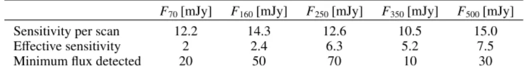
Table 1. Sensitivity of the Herschel observations used in this study.
F70[mJy] F160[mJy] F250[mJy] F350[mJy] F500[mJy] Sensitivity per scan 12.2 14.3 12.6 10.5 15.0 Effective sensitivity 2 2.4 6.3 5.2 7.5
Minimum flux detected 20 50 70 10 30
by Andrews et al.(2011) with the Sub-Millimeter Array (Ho et al. 2004). Recent work with ALMA (Wootten & Thompson 2009) has achieved new results in the field as seen in works by van der Marel et al. (2013) and the recent study on the transi-tional disk HL Tauri (ALMA Partnership et al. 2015).
The aim of this work is to study the young stellar objects (YSOs) in the Ophiuchus star-forming region. Herschel data provide us with accurate fluxes of the detected objects, and en-ables the construction of the spectral energy distributions (SEDs) along with other multi-wavelength photometric data, collected byRibas et al.(2014). The study of the SEDs also allows us to classify the transitional disks in the region by identifying the pre-viously mentioned lack of excess in near and/or mid-IR region.
The structure of this work is as follows: Sect. 2 describes the Herschelobservations and data reduction, explaining the source detection and photometry extraction processes. In Sect. 3 we ex-plain the results obtained from the data reduction, both with the method described inRibas et al.(2013) and with the analysis of the SED of each individual object. In Sect. 4 we discuss the de-tection statistics and compare them with other similar studies. In Sect. 5 we present the conclusions of this work.
2. Observations and data reduction
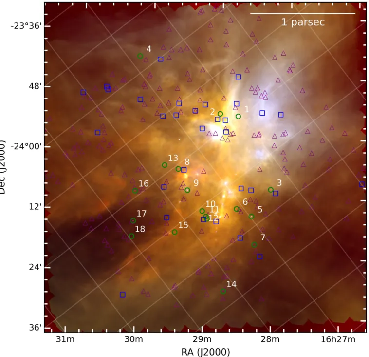
The Ophiuchus cloud complex was observed by Herschel as part of the Herschel Gould Belt Survey (André et al. 2010) and by a deeper PACS survey (Alves de Oliveira et al. 2013). It is one of the closest star-forming regions, located at an estimated distance of 130 pc and with an age between 2 and 5 Myr, although it has been suggested that it is younger (seeWilking et al. 2008, for a review on the region). Apart from its proxmity, most significant characteristic of this cloud is its dense core, which is the focus of our study. The cloud itself appears as a large scale structure with complex filaments, heated by B-type stars, and is strongly emitting at infrared wavelengths. We might consider the cloud itself as a possible source of contamination. Figure1shows the region with the objects in the sample overplotted and marked differently according to their state of non-detected, detected, or transitional.
The maps used to examine this region were obtained from two sets of observations, using the parallel mode of both PACS (Poglitsch et al. 2010) and SPIRE (Griffin et al. 2010) on board the Herschel Space Observatory. For SPIRE maps (250 µm, 350 µm and 500 µm) the parallel mode was used, with a speed of 6000/s (program KPGT_pandre_1), but for the PACS maps (70 µm and 160 µm) the scan mapping mode was used, with a cross-scan speed of 2000/s (program OT1_pabraham_3). We used this later PACS data because it goes deeper, as shown by the sensitivity limits given in the SPIRE/PACS Observers’ Manual and in Table1in this work. In both cases (PACS and SPIRE), a single pair of scan and cross-scan was obtained. The obsids for the SPIRE maps are (1342-) 205093 and 205094, and for PACS maps (1342-) 238816 and 238817.
The maps were produced using Scanamorphos (Roussel 2013), an IDL software designed to process Herschel maps. Version 24.0 was used for PACS maps, with calibration file
version 65, and version 22.0 for SPIRE maps, with calibration files version 12.3.
2.1. Sample selection and point source photometry
The objective of this work is to determine the nature of the sources detected in the maps produced with PACS and SPIRE observations and to obtain fluxes in the mid- to far-IR re-gions when detected. The YSO candidates were selected from the work of Ribas et al. (2014) (which for Ophiuchus con-tains objects from Natta et al. 2002; Wilking et al. 2005; Alves de Oliveira et al. 2010; Erickson et al. 2011), for hav-ing known spectral type from spectroscopy, makhav-ing a list of 258 sources, all of them located in the core of the cloud. For a more complete study, the objects fromCieza et al.(2010) con-tained in the region of interest were also considered. The final sample consists of 261 objects. We used photometry from the 2MASS K-band (Skrutskie et al. 2006) and WISE4 (Wright et al. 2010) to classify the disks according to the method described by Lada(1987). The only object that does not fulfill the criteria is IRS 48, which has a positive slope that is almost flat. This object cannot be classified as Class I and remains Class II in the final classificaiton because of the lack of strong emission in mid- and far-IR.
To determine whether our candidates are transitional disks or not, the first step was to detect sources in our maps and extract the photometry from them. We used the algorithm Sussextractor in the Herschel interactive processing environment (HIPE), ver-sion 12.1, with a threshold of S /N > 3. Additionally, visual in-spection was applied to all sources. Only sources clearly sepa-rated from filaments and distinguishable from the background were selected as valid detections.
We extracted aperture photometry for these sources using the sourceExtractorDaophot task in HIPE (Ott 2010). The fluxes were aperture corrected to account for the shape of the PSF and they are listed in Table4. Those corrections were obtained from Balog et al.(2014) for PACS and from the SPIRE Observers’ Manual (now named SPIRE Handbook) version 2.5. In Table4, objects marked with an asterisk suffered from high nearby back-ground emission and, in those cases, we used a special sky es-timate from a rectangular area identified after visual inspection. The set of apertures and the corrections applied to the photom-etry extracted are shown in Table 2. We tested several point-source extraction algorithms, including Sussextractor, Daophot, AnnularSkyAperturePhotometry, and Hyper (Traficante et al. 2015), and different apertures. The combination above provides the best fit to the MIPS70 (Rieke et al. 2004) fluxes of clean selected sources in the field.
At the end of the process, we had 49 successfully detected sources in at least one PACS band, and 19 in a SPIRE band; PACS also detected all of these. Images of the detected objects can be found in Fig.A.2, for visual inspection.
The calibration errors for PACS and SPIRE are 5% and 7% (as stated in the PACS Observer’s Manual, version 2.3 and in the SPIRE Observer’s Manual version 2.5), however, as a more conservative estimation, we used 25% for both. These measurement uncertainties account for the high variations in the
Fig. 1.RGB image (PACS 70 in blue, PACS 100 in green, and PACS 160 in red) of the observed Ophiuchus region with the marked objects. Transitional disks are marked with green circles. The blue squares mark the detected objects, and the purple triangles mark the rest of the sample of known young stars in the region.
results of the different extraction methods and apertures listed above.
In Table3we show the parameters of the detected sources, as given in the literature, and for an easier reference we list the identification numbers (ID) used in this work as seen in Fig.1. From now on, the ID number is referenced in parenthesis for its respective source. Table 4 gives the fluxes measured with Herschelfor each source.
2.2. Sensitivity and non-detections
The high background present in the region increases the sen-sitivity limit of these observations, and affects the number of
detections. In Table1 we present the sensitivities given in the SPIRE/PACS Parallel Mode Observers’ Manual v2.1 (Sect. 2.3), and the minimum flux detected for each band. Also, the effective sensitivity is calculated taking the number of scans made per map into account; this includes six for the PACS maps and two for the SPIRE maps. We also report a lower value of fluxes in the cleanest areas of the map, which agrees with the fact that the ex-tended emission from the molecular cloud reduces the effective sensitivity.
Another study took into account the sources detected by Spitzerand catalogued by c2d (Evans et al. 2009) in each of the apertures defined per band and per detected source to estimate possible contamination due to Herschel resolution. The flux in
Table 2. Aperture photometry parameters. Band FWHM(00
) Radius (00
) Inner annulus (00
) Outer annulus (00
) Aperture correction factors
PACS-70 5.4 6 25 35 1.5711
PACS-160 10.5 12 25 35 1.4850
SPIRE-250 18 22 60 90 1.2584
SPIRE-350 24 30 60 90 1.2242
SPIRE-500 36 42 60 90 1.1975
Table 3. Parameters of detected sources as extracted from the literature.
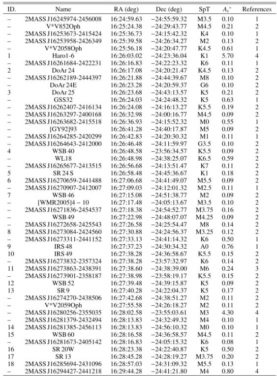
ID. Name RA (deg) Dec (deg) SpT Av∗ References – 2MASS J16245974-2456008 16:24:59.63 −24:55:59.32 M3.5 0.10 1 – V*V852Oph 16:25:24.38 −24:29:43.77 M4.5 0.21 2 – 2MASS J16253673-2415424 16:25:36.73 −24:15:42.32 K4 0.10 1 – 2MASS J16253958-2426349 16:25:39.58 −24:26:34.27 M2 0.13 2 – V*V2058Oph 16:25:56.18 −24:20:47.77 K4.5 0.61 1 1 Haro1-6 16:26:03.02 −24:23:36.04 K1 5.70 4 – 2MASS J16261684-2422231 16:26:16.83 −24:22:23.32 K6 0.11 1 2 DoAr 24 16:26:17.08 −24:20:21.47 K4.5 0.13 2 – 2MASS J16262189-2444397 16:26:21.88 −24:44:39.67 M8 0.10 2 – DoAr 24E 16:26:23.28 −24:20:59.37 G6 0.10 2 3 DoAr 25 16:26:23.68 −24:43:13.57 K5 0.21 2 – GSS32 16:26:24.03 −24:24:48.32 K5 0.63 1 – 2MASS J16262407-2416134 16:26:24.08 −24:16:13.27 K5.5 0.19 2 – 2MASS J16263297-2400168 16:26:32.98 −24:00:16.77 M4.5 0.09 2 – 2MASS J16263682-2415518 16:26:36.93 −24:15:52.32 M0 0.55 1 – [GY92]93 16:26:41.28 −24:40:17.87 M5 0.09 2 – 2MASS J16264285-2420299 16:26:42.83 −24:20:30.32 M1 0.11 1 – 2MASS J16264643-2412000 16:26:46.48 −24:11:59.97 G3.5 0.10 2 4 WSB 40 16:26:48.58 −23:56:34.57 K5.5 0.09 2 – WL18 16:26:48.98 −24:38:25.07 K6.5 0.59 2 – 2MASS J16265677-2413515 16:26:56.68 −24:13:51.47 K7 0.11 2 5 SR 24 S 16:26:58.48 −24:45:36.67 K1 0.18 2 6 2MASS J16270659-2441488 16:27:06.68 −24:41:49.07 M5.5 0.09 2 – 2MASS J16270907-2412007 16:27:09.03 −24:12:01.32 M2.5 0.11 1 7 WSB 46 16:27:15.08 −24:51:38.77 M2 0.09 2 – [WMR2005]4 − 10 16:27:17.48 −24:05:13.67 M3.5 0.10 2 – 2MASS J16271836-2454537 16:27:18.38 −24:54:52.77 M3.75 0.16 2 – WSB 49 16:27:22.98 −24:48:07.07 M4.25 0.09 2 – 2MASS J16272658-2425543 16:27:26.58 −24:25:54.47 M8 0.14 2 8 2MASS J16273084-2424560 16:27:30.88 −24:24:56.37 M3.25 0.12 2 – 2MASS J16273311-2441152 16:27:33.13 −24:41:14.32 K6 0.50 1 9 IRS 48 16:27:37.23 −24:30:34.32 A0 0.76 1 10 IRS 49 16:27:38.28 −24:36:58.67 K5.5 0.15 2 – 2MASS J16273832-2357324 16:27:38.28 −23:57:32.97 K6 0.14 2 11 2MASS J16273863-2438391 16:27:38.60 −24:38:39.00 M6 0.24 3 – 2MASS J16273901-2358187 16:27:38.98 −23:58:19.17 K5.5 0.15 2 12 WSB 52 16:27:39.48 −24:39:15.87 K5 0.09 2 13 SR 9 16:27:40.28 −24:22:04.37 K5 0.17 2 – 2MASS J16274270-2438506 16:27:42.68 −24:38:51.27 M2 0.11 2 – V*V2059Oph 16:27:55.58 −24:26:18.27 M2 0.11 2 – 2MASS J16280256-2355035 16:28:02.58 −23:55:03.61 M3 4.30 4 – 2MASS J16281379-2432494 16:28:13.83 −24:32:49.32 M4 0.10 1 14 2MASS J16281385-2456113 16:28:13.83 −24:56:10.32 M0 0.10 1 15 WSB 60 16:28:16.58 −24:36:58.57 M4.5 0.11 2 – 2MASS J16281673-2405142 16:28:16.83 −24:05:15.32 K6 0.08 1 16 SR 20W 16:28:23.38 −24:22:40.87 K5 0.50 2 17 SR 13 16:28:45.28 −24:28:19.27 M3.75 0.20 2 18 2MASS J16285694-2431096 16:28:57.03 −24:31:09.32 M5.5 0.13 1 – 2MASS J16294427-2441218 16:29:44.28 −24:41:21.80 M4 0.80 4 Notes. Also, we give the ID number used to identify the transitional disks.(∗)All A
vare calculated according toRibas et al.(2014). References. 1)Erickson et al.(2011); 2)Wilking et al.(2005); 3)Natta et al.(2002); 4)Cieza et al.(2010).
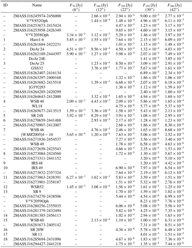
Table 4. Point source fluxes of each of the 49 sources detected.
ID Name F70[Jy] F160[Jy] F250[Jy] F350[Jy] F500[Jy]
– 2MASS J16245974-2456008 0.05 ± 0.01 – – – – – V*V852Oph 0.73 ± 0.18 – – – – – 2MASS J16253673-2415424 0.74 ± 0.18 – – – – – 2MASS J16253958-2426349 0.92 ± 0.23 – – – – – V*V2058Oph 3.86 ± 0.97 3.77 ± 0.94 12.56 ± 3.14 – – 1 Haro1-6 10.70 ± 2.68 7.48 ± 1.87 – – – – 2MASS J16261684-2422231 0.20 ± 0.05 – – – – 2 DoAr 24 0.50 ± 0.12 – – – – – 2MASS J16262189-2444397 0.10 ± 0.02 – – – – – DoAr 24E 4.17 ± 1.04 3.91 ± 0.98 – – – 3 DoAr 25 1.39 ± 0.35 3.52 ± 0.88 4.17 ± 1.04 5.30 ± 1.33 2.05 ± 0.51 – GSS32 3.70 ± 0.93 – – – – – 2MASS J16262407-2416134 3.04 ± 0.76 6.10 ± 1.53 4.73 ± 1.18 2.66 ± 0.66 1.12 ± 0.28 – 2MASS J16263297-2400168 0.08 ± 0.02 0.13 ± 0.03 – 0.01 ± 0.00 – – 2MASS J16263682-2415518* 1.37 ± 0.34 0.72 ± 0.18 0.44 ± 0.11 – – – [GY92]93 0.02 ± 0.00 – – – – – 2MASS J16264285-2420299 0.65 ± 0.16 – – – – – 2MASS J16264643-2412000 0.57 ± 0.14 – – – – 4 WSB 40 0.42 ± 0.10 0.29 ± 0.07 – – – – WL18 0.42 ± 0.10 – – – – – 2MASS J16265677-2413515 0.21 ± 0.05 0.79 ± 0.20 – – – 5 SR42S 9.70 ± 2.42 7.88 ± 1.97 5.06 ± 1.26 3.02 ± 0.76 1.55 ± 0.39 6 2MASS J16270659-2441488 0.10 ± 0.02 – – – – – 2MASS J16270907-2412007 0.07 ± 0.02 0.23 ± 0.06 – 0.11 ± 0.03 – 7 WSB 46 0.25 ± 0.06 0.15 ± 0.04 – – – – [WMR2005]4-10 0.18 ± 0.04 0.32 ± 0.08 0.51 ± 0.13 0.37 ± 0.09 – – 2MASS J16271836-2454537* 0.07 ± 0.02 0.05 ± 0.01 0.07 ± 0.02 – – – WSB 49 0.04 ± 0.01 – – – – – 2MASS J16272658-2425543 0.04 ± 0.01 – – – – 8 2MASS J16273084-2424560 0.50 ± 0.13 – – – – – 2MASS J16273311-2441152 1.27 ± 0.32 0.08 ± 0.02 – – – 9 IRS48 37.57 ± 9.39 12.85 ± 3.21 6.48 ± 1.62 2.51 ± 0.63 – 10 IRS49* 1.29 ± 0.32 0.95 ± 0.24 0.07 ± 0.02 0.67 ± 0.17 – – 2MASS J16273832-2357324* 0.63 ± 0.16 0.25 ± 0.06 0.52 ± 0.13 0.30 ± 0.07 – 11 2MASS J16273863-2438391 0.09 ± 0.02 – – – – – 2MASS J16273901-2358187 0.44 ± 0.11 0.52 ± 0.13 0.10 ± 0.02 0.09 ± 0.02 0.03 ± 0.01 12 WSB 52* 2.37 ± 0.59 2.23 ± 0.56 3.43 ± 0.86 0.76 ± 0.19 0.28 ± 0.07 13 SR 9 0.86 ± 0.21 0.22 ± 0.05 – – – – 2MASS J16274270-2438506 0.02 ± 0.01 – – – – – V*V2059Oph 0.06 ± 0.01 – – – – – 2MASS J16280256-2355035 0.02 ± 0.01 – – – – – 2MASS J16281379-2432494 0.05 ± 0.01 – – – – 14 2MASS J16281385-2456113 0.74 ± 0.18 0.68 ± 0.17 0.29 ± 0.07 0.19 ± 0.05 0.14 ± 0.03 15 WSB 60 0.87 ± 0.22 1.19 ± 0.30 1.26 ± 0.32 1.79 ± 0.45 – – 2MASS J16281673-2405142 0.12 ± 0.03 – – – – 16 SR 20W 0.89 ± 0.22 0.60 ± 0.15 0.57 ± 0.14 0.46 ± 0.12 0.37 ± 0.09 17 SR 13 1.36 ± 0.34 1.32 ± 0.33 0.79 ± 0.20 0.51 ± 0.13 0.20 ± 0.05 18 2MASS J16285694-2431096 0.02 ± 0.01 – – – – – 2MASS J16294427-2441218 0.05 ± 0.01 – – – –
Notes.(∗)Sources near bright background emission; sky measurement was done in clean regions.
MIPS-24 band of each of this c2d sources was used to extrapo-late via the median SED of the Ophiuchus region (see Table5) the expected fluxes at 70 µm. In TableA.1, we list a sum of all the expected fluxes for this contaminating sources, where it is possible to check whether the expected contamination is lower than the flux error. Notice that this contamination flux is only an estimation, as only the reported object has been detected in the aperture.
3. Results
The fluxes of all the detected sources per band are given in Table4, as mentioned above. As expected, the higher flux corre-sponds to the most known object in the region, IRS 48 (#9). All the objects proposed as transitional disk candidates present rela-tively high fluxes, being 2MASS J16285694-2431096 (#18) the candidate with the lower flux at 70 µm (20 mJy). The detection
on more than one band for these objects seems to be arbitrary. Less than half of the candidates have been detected either in one band or in all of them. This is probably related to the physical properties of each of the disks rather than to instrumental issues.
3.1. Identification of transitional disks
Once we measured the fluxes, we use the criterion byRibas et al. (2013) to classify transitional disks with Herschel photometry. As previously noted, transitional disks display little or no excess at near- to mid-IR, and large excess at long wavelengths, which translates into a change of slope in the SED of the object around 12 µm, i.e. from a negative to positive slope. To proceed with the identification, we defined two indexes , following:
αλ1−λ2=
log(λ1Fλ1) − log(λ2Fλ2)
log(λ1) − log(λ2)
, (1)
where λ is measured in µm and Fλin erg s−1cm−2. The first in-dex is defined for the band K acquired from 2MASS and 12 µm acquired from WISE. The second index is defined for the 12 µm band and the 70 µm band acquired from Herschel. The criterion to determine whether an object is a transitional disk candidate is α12−70> 0, since we define transitional disks as objects with
a deficit of excess flux at near- to mid-IR fluxes, but standard excesses at longer wavelengths. For DoAr 24 (#2), the 12 µm-band was not available and, therefore, we used 8 µm µm-band from Spitzer/IRAC (Fazio et al. 2004) instead.
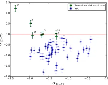
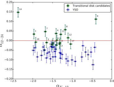
To understand the result of this process, we represent in Fig. 2 a slope-slope diagram, which shows the value of the two different slopes in the two axes. The figure shows that we obtained two candidates with a positive slope between 12 µm and 70 µm, clearly separated from the Class II population. These two candidates, 2MASS J16281385-2456113 (#14) and Haro1-6 (#1), clearly fulfil the criteria of having a lack of mid-IR excess since Haro1-6 (#1) is an object previously classified as debris disk in Cieza et al. (2010). The candidate 2MASS J16281385-2456113 (#14), has never been reported before as a transitional disk. The other objects above the threshold do not have this kind of clear 12 µm flux deficit, which is indicative of the presence of a flatter slope in the mid- to far-infrared wave-lengths. If we construct the SEDs of those objects (see Fig. 4), we see that in general they do not present the characteristic gap expected from a transitional disk. However, as they fulfil the criteria, we classified them here as tentative candidates. Some of these candidates were also classified as transitional disks in previous works. Object WSB 60 (#15) was imaged inAndrews et al.(2009), detecting a small inner hole in dust continuum ob-servations done with the Sub-Millimeter Array (Ho et al. 2004). In the work by Cieza et al.(2010) DoAr 25 (#3) was already suggested as a candidate. We consider objects SR 42 S (#5), WSB 46 (#7), and SR 20 W (#16) as tentative candidates de-spite they do not fulfill the criteria for their nominal values, but we are considering a high error in PACS photometry. In particu-lar, SR 42 S (#5) has already been classified as transitional disk, and appears in Espaillat et al. (2014) as so. For WSB 46 (#7) and SR 20 W (#16), further study is needed to determine their nature.
3.2. Complementary identification with spectral energy distributions
To better analyse the nature of these objects, we built their SEDs using data from optical to mid-infrared from both ground-based and space telescopes (all references for the photometry can be
2.5 2.0 1.5 1.0 0.5 0.0
α
K−
12 2.0 1.5 1.0 0.5 0.0 0.5 1.0 1.5α
12− 70 1 3 5 7 14 15 16Transitional disk candidates YSO
Fig. 2.SED slope between 12 and 70 µm as a function of the SED slope between the K-band and 12 µm. Transitional disks are marked with green squares.
Table 5. Median SED of detected disks in Ophiuchus.
Band Median First quartile Third quartile Detections
J 1.0000 1.0000 1.0000 49 H 0.6109 0.5664 0.6577 49 K 0.3305 0.3018 0.3662 49 IRAC-3.6 0.0743 0.0628 0.0958 45 IRAC-4.5 0.0380 0.0305 0.0537 47 IRAC-5.8 0.0212 0.0162 0.0293 46 IRAC-8.0 0.0121 0.0088 0.0190 48 MIPS-24 0.0018 0.0013 0.0030 48 PACS-70 0.0003 0.0001 0.0008 49 PACS-160 8.53 × 10⁻⁵ 5.54 × 10⁻⁵ 0.0002 26 SPIRE-250 3.48 × 10⁻⁵ 2.32 × 10⁻⁵ 0.0001 17 SPIRE-350 9.60 × 10⁻⁶ 5.88 × 10⁻⁶ 1.44 × 10⁻⁵ 15 SPIRE-500 2.62 × 10⁻⁶ 2.12 × 10⁻⁶ 4.18 × 10⁻⁶ 8
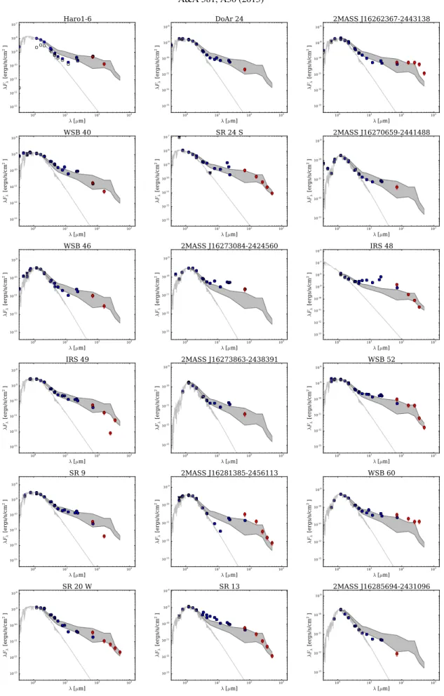
found in Sect. 2.1). We completed these SEDs with the photome-try shown in Table2and extracted from Herschel data, therefore, we cover a range between 0.35 to 500 µm. Figures4 andA.1 show the obtained SEDs, plus the NextGen atmosphere model for each object (Hauschildt et al. 1999), which are the best ap-proximation of how a naked photosphere would emit as a func-tion of its spectral type.
We also built the median SED of all the objects detected in the region for comparison (see Table5), which is plotted along each object’s SEDs. Because of the lack of detections for fluxes under the sensitivity limits given in Table4, the median SED might be slightly overestimated, but we assume the effect in our result is negligible.
To determine the interstellar extinction, we used the pro-cedure in Ribas et al. (2014) and the extinction law from Weingartner & Draine(2001), which uses a model of grains to estimate the interstellar extinction, scattering, and infrared emis-sion. In each plot of Figs.4andA.1, the observed fluxes are also shown as empty circles. The de-reddened fluxes, according to the associated interstellar extinction, are shown as filled circles. When visually inspecting the SEDs, we detect objects with a lack of mid-IR excess that were not classified as transitional disks, according to the criteria ofRibas et al.(2013) described in Sect. 3.1. Some of these objects are well known in the literature, such as IRS 48 (#9). To make a more reliable study of the region,
2.5 2.0 1.5 1.0 0.5 0.0
α
K−
12 0.20 0.15 0.10 0.05 0.00 0.05 0.10 0.15 0.20α
12 − 24 1 2 3 4 6 7 8 9 10 11 12 13 14 15 16 17 18Transitional disk candidates YSO
Fig. 3.SED slope between 12 and 24 µm as a function of the SED slope between the K-band and 12 µm. Transitional disks are marked with green squares.
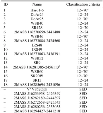
we add in this subsection a complementary criterion based on Spitzerdata to identify the other transitional disks or transitional disks candidates detected by Herschel with a change of slope between 12 µm and 24 µm. Figure3shows the new slope-slope diagram.
We detected 17 transitional disks candidates with this crite-ria. Six of the objects detected with the previous criteria appear now as well, with the exception of SR 24 S (#5), which is a con-firmed transitional disk.
Figure4shows the SEDs for the 18 transitional disks can-didates, where the change of slope is not equally noticeable for all of them. In the case of 2MASS J16281385-2456113 (#14), the change of slope is evident, in agreement with that expected from the slope-slope diagram. In cases such as WSB 60 (#15) or IRS 48 (#9), which are well-known transitional disks, the slope is flatter, and located in a different position in the wavelength axis. For SR 24 S (#5), we see an unexpected behaviour, where we get a discrepancy between MIPS-24 and WISE4 fluxes, but we still see an increase in the far-IR emission with respect to the near-IR. Another object classified as a transitional disk in Cieza et al.(2010) is SR 9 (#13), although it has a continuous decreasing slope, as the criterion shows, and looks more like a Class II SED. The rest of the objects in the sample have been widely studied, but not previously considered transitional disks. The variation in the outputs of both methods illustrates the com-plexity in defining a selection criteria.
4. Discussion
4.1. Detection statistics
The initial sample was composed of 261 YSO objects in the centre of Ophiuchus, with known spectral type from optical spectroscopy and all classified as Class II objects. Our sam-ple is different from that in Evans et al. (2009), since they had photometrically selected objects, including many objects with other classes, while we have only spectroscopically con-firmed Class II YSOs. All of these YSOs fell within the cov-erage of the maps used, and 49 were detected in at least one Herschelband, 49 in PACS, and 19 in SPIRE. This leads to a Herscheldetection rate of 18.77%±2.6%, which is much smaller than the percentage of detections obtained in similar studies in
Chamaeleon (Ribas et al. 2013) and Lupus (Bustamante et al. 2015) of around 30%. Given that Ophiuchus is closer than those regions (150 ∼ 200 pc), the low detection rate is probably due to the higher background, which is emitting at mid- and long-IR wavelengths, and precludes the detection of faint objects.
4.2. Incidence of transitional disks in the centre of Ophiuchus We report here the detection of 18 transitional disk candidates in the cloud complex in the centre of Ophiuchus based on new Herschel and previous known data of spectroscopically con-firmed YSO sample. Despite the fact that all of these objects fulfil either one or both of the criteria exposed previously, only a few of them have evident changes of slopes in the SEDs. The candidate with the biggest change in slope, 2MASS J16281385-2456113 (#14), is new to the literature.
The fraction of transitional disk candidates observed in Ophiuchus based on our Herschel sample, is 37%+7−6. We have considered two classification criteria, depending on the change of slope, that is, on the wavelength position of the lack of mid-IR excess. If we only consider our main criteria, the fraction is lower, at 14%+6−4, but it is compatible with the fractions measured in other regions with similar ages in previous works (Espaillat et al. 2014). Even though we have identified 18 transitional disks candidates in total, some of them present a relatively flat slope and, in the slope-slope diagram, are represented very close to, or even below, the threshold . Having objects with nearly a Class-II slope explains the high fraction of transitional disks in the re-gion, as many of them might be fulfilling the criteria due to the large error in their PACS fluxes. These objects would need fur-ther study for their safe classification. One of the objects close to the threshold, however, namely YLW 58 or WSB 60 (#15), had been imaged with SMA and shows a small but conspicuous in-ner hole (Andrews et al. 2011). Despite this, most of the objects in the first criterion were also detected by the complementary criterion; SR 42 S (#5) was not, even though it is a confirmed transitional disk (Andrews et al. 2011). The fact that Herchel data is including transitional candidates to the sample, confirms the improvement that Herschel represents regarding reaching to further regions in disks. The longer wavelengths now accessi-ble allow us to detect wider and larger cavities, which we could not have identified solely with data from Spitzer at mid-infrared ranges.
4.3. Other interesting objects
Even though we have combined two criteria to identify new can-didates, and that these criteria select even very small changes of slope, there might be objects in the sample with the characteris-tics of a transitional disk, which are, as previously noted, a lack of excess around 10 µm and normal excesses at mid- to far-IR. If we inspect Fig.A.1, we observe that several objects present these features. There are two clear cases of objects previously classified as transitional disk candidates: 2MASS J16280256-2355035 and 2MASS J16294427-2441218. Both of these candi-dates present a lack of excess around 8 µm and excesses in longer wavelengths, but because of the restrictions in the criteria, nei-ther appear as transitional candidates. The objects V* V852 Oph, 2MASS J16253958-2426349 and 2MASS J16262189-2444397 are similar cases that were never classified as transitional disks, but have a gap in their SED, which could be an indication of a hole in their disks. The object 2MASS J16272658-2425543 also shows a lack of excess around 10 µm with a larger excess in
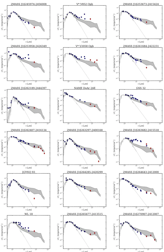
Fig. 4.Spectral energy distribution (SED) of the sources classified as transitional disks candidates. Blue dots show data acquired from the literature, red dots are photometric fluxes obtained from Herschel data. Grey dashed line is the photosphere model according to the spectral type, and the grey shaded area is the filled area between the first and third quartile of all the disk fluxes. Observed fluxes are shown with empty circles and Avvalues used are in Table3.
Table 6. Summary of all transitional disk candidates in Ophiuchus. ID Name Classification criteria
1 Haro1-6 12−70∗ 2 DoAr24 12−24 3 DoAr25 12−70∗ 4 WSB40 12−24 5 SR42S 12−70 6 2MASS J16270659-2441488 12−24 7 WSB46 12−70∗ 8 2MASS J16273084-2424560 12−24 9 IRS48 12−24 10 IRS49 12−24 11 2MASS J16273863-2438391 12−24 12 WSB52 12−24 13 SR9 12−24 14 2MASS J16281385-2456113† 12−70∗ 15 WSB60 12−70∗ 16 SR20W 12−70∗ 17 SR13 12−24 18 2MASS J16285694-2431096 12−24 – V∗ V852Oph SED – 2MASS J16253958–2426349 SED – 2MASS J16262189–2444397 SED – 2MASS J16272658–2425543 SED – 2MASS J16280256–2355035 SED – 2MASS J16294427-2441218 SED
Notes.(∗)These objects have also been classified with the complemen-tary criterion of 12–24.(†)This transitional disk candidate is new to the literature.
longer wavelengths. This object could also be considered a tran-sitional candidate, despite the fact that it does not fulfil any of the criteria. All of these objects are shown in Table6along with the previous objects classified as transitional disk candidates.
4.4. Study of 70 micron fluxes in transitional disks
For a comparison of the 70 µm flux of both the transitional disk candidates and tentative candidates, we constructed the median SED of all the detected objects in the sample, using the photo-metric data in Table5. This would show if, apart from a lack of excess in the near mid-IR, transitional disks also show another remarkable characteristic that could be used in classification or, possibly, in disk modelling. The median SED lacks the contri-bution from the faintest objects, which might remain undetected by Herschel or some of the other surveys, and hence is just an upper limit to the true median SED of Ophiuchus.
When we overplot the median SED to the detected fluxes (as a grey shaded area in Figs. 4 andA.1), we only find the 70 µm flux to be higher for some of the objects classified as transitional disks candidates. Hence, we cannot conclude that we have detected a trend in the transitional disk population, such as has been observed in previous investigations (Ribas et al. 2013,Bustamante et al. 2015). We also find the case of 2MASS J16285694-2431096 (#18), where the 70 µm flux is not only lower than the median SED, but lower than the third quartile. Because of the lack of large excess in mid- to far-IR and the fact that this object presents a slightly smaller flux in the 70 µm band than the rest of transitional disks candidates, it needs fur-ther study to clarify its nature.
5. Conclusions
We have detected 49 objects in the central region of Ophiuchus in at least one PACS band and 19 in at least one SPIRE band. We obtained accurate photometric fluxes for the detected objects by means of aperture photometry.
Seven of the detected objects were classified as transitional disk candidates by the criterion in Ribas et al. (2013), and 11 more were classified according to the complementary cri-terion, generating a total sample of 18 transitional disk candi-dates. Some of these candidates were already imaged in previous works, and hence, confirmed. Six more objects are added to the final classification of candidates that have transitional features in their SEDs, rather than fulfilling any of the criterion. All of the transitional disk candidates are shown in Table6along with their classification criteria. This large difference between the identifi-cation methods can be due to the different nature or evolutionary stages of the disks, creating different geometries and leading to a large diversity of SEDs.
Several of the objects classified as transitional disks can-didates have not been considered cancan-didates before, but 2MASS J16281385-2456113 (#14) appears to be an attractive object for follow-up because of its prominent change of slope when compared to the rest of the sample, including previously imaged disks, such as IRS 48 (#9).
So far, Herschel data has proved to be very useful to improve the characterization of the outer regions of protoplanetary sys-tems because of its long-wavelength coverage, unattainable un-til now, and its improved sensitivity and spatial resolution com-pared with previous IR missions. A study of the SED population of the disk sample detected with Herschel should give us more information on the true nature of these disks, but this study is outside the scope of this work.
Acknowledgements. We thank the referee for his/her constructive comments. This work has been possible thanks to the ESAC Space Science Faculty for funding with code ESAC-321, ESAC Traineeship program and of the Herschel Science Centre. We thank Gábor Marton for useful discussions on Herschel data evaluation. This work was partly supported by the Hungarian research grant OTKA 101393, and by the Momentum grant of the MTA CSFK Lendület Disk Research Group. PACS was developed by a consortium of institutes led by MPE (Germany), including UVIE (Austria); KUL, CSL, IMEC (Belgium); CEA, OAMP (France); MPIA (Germany); IFSI, OAP/AOT, OAA/CAISMI, LENS, SISSA (Italy); IAC (Spain). This development has been supported by the funding agencies BMVIT (Austria), ESA-PRODEX (Belgium), CEA/CNES (France), DLR (Germany), ASI (Italy), and CICT/MCT (Spain). SPIRE was developed by a consortium of institutes led by Cardiff Univ. (UK), including Univ. Lethbridge (Canada); NAOC (China); CEA, LAM (France); IFSI, Univ. Padua (Italy); IAC (Spain); Stockholm Observatory (Sweden); Imperial College London, RAL, UCL-MSSL, UKATC, Univ. Sussex (UK); and Caltech, JPL, NHSC, Univ. Colorado (USA). This development has been supported by national funding agencies: CSA (Canada); NAOC (China); CEA, CNES, CNRS (France); ASI (Italy); MCINN (Spain); SNSB (Sweden); STFC (UK); and NASA (USA).This study also makes use of the data products from the Two Micron All Sky Survey (2MASS), a joint project of the University of Massachusetts and IPAC/Caltech, funded by NASA and the National Science Foundation; data products from the Wide-field Infrared Survey Explorer (WISE), a joint project of the University of California, Los Angeles, and the Jet Propulsion Laboratory (JPL)/California Institute of Technology (Caltech); data products from DENIS, a project partly funded by the SCIENCE and the HCM plans of the European Commission under grants CT920791 and CT940627; the NASA Infrared Processing and Analysis Center (IPAC) Science Archive; and the SIMBAD database.
References
ALMA Partnership, Brogan, C. L., Perez, L. M., et al. 2015,ApJ, 808, L3
Alves de Oliveira, C., Moraux, E., Bouvier, J., et al. 2010,A&A, 515, A75
Alves de Oliveira, C., Ábrahám, P., Marton, G., et al. 2013,A&A, 559, A126
Andrews, S. M., Wilner, D. J., Hughes, A. M., Qi, C., & Dullemond, C. P. 2009,
ApJ, 700, 1502
Andrews, S. M., Wilner, D. J., Espaillat, C., et al. 2011,ApJ, 732, 42
Balog, Z., Müller, T., Nielbock, M., et al. 2014,Exp. Astron., 37, 129
Bustamante, I., Merín, B., Ribas, Á., et al. 2015,A&A, 578, A23
Cieza, L. A., Schreiber, M. R., Romero, G. A., et al. 2010,ApJ, 712, 925
Clarke, C. J., Gendrin, A., & Sotomayor, M. 2001,MNRAS, 328, 485
Dullemond, C. P., & Dominik, C. 2005,A&A, 434, 971
Erickson, K. L., Wilking, B. A., Meyer, M. R., Robinson, J. G., & Stephenson, L. N. 2011,AJ, 142, 140
Espaillat, C., Muzerolle, J., Najita, J., et al. 2014, in Protostars ans Planets VI, eds. R. S. Klessen, C. P. Dullemond & T. Henning (Tucson: University of Arizona Press), 497
Evans, II, N. J., Dunham, M. M., Jørgensen, J. K., et al. 2009,ApJS, 181, 321
Fazio, G. G., Hora, J. L., Allen, L. E., et al. 2004,ApJS, 154, 10
Griffin, M. J., Abergel, A., Abreu, A., et al. 2010,A&A, 518, L3
Hauschildt, P. H., Allard, F., & Baron, E. 1999,ApJ, 512, 377
Ho, P. T. P., Moran, J. M., & Lo, K. Y. 2004,ApJ, 616, L1
Kim, K. H., Watson, D. M., Manoj, P., et al. 2013,ApJ, 769, 149
Lada, C. J. 1987, in Star Forming Regions, eds. M. Peimbert, & J. Jugaku,IAU Symp., 115, 1
Marsh, K. A., & Mahoney, M. J. 1992,ApJ, 395, L115
Natta, A., Testi, L., Comerón, F., et al. 2002,A&A, 393, 597
Ott, S. 2010, in Astronomical Data Analysis Software and Systems XIX, eds. Y. Mizumoto, K.-I. Morita, & M. Ohishi,ASP Conf. Ser., 434, 139
Pilbratt, G. L., Riedinger, J. R., Passvogel, T., et al. 2010,A&A, 518, L1
Poglitsch, A., Waelkens, C., Geis, N., et al. 2010,A&A, 518, L2
Ribas, Á., Merín, B., Bouy, H., et al. 2013,A&A, 552, A115
Ribas, Á., Merín, B., Bouy, H., & Maud, L. T. 2014,A&A, 561, A54
Rieke, G. H., Young, E. T., Engelbracht, C. W., et al. 2004,ApJS, 154, 25
Roussel, H. 2013,PASP, 125, 1126
Skrutskie, M. F., Cutri, R. M., Stiening, R., et al. 2006,AJ, 131, 1163
Strom, K. M., Strom, S. E., Edwards, S., Cabrit, S., & Skrutskie, M. F. 1989,AJ, 97, 1451
Traficante, A., Fuller, G. A., Pineda, J. E., & Pezzuto, S. 2015,A&A, 574, A119
van der Marel, N., van Dishoeck, E. F., Bruderer, S., et al. 2013,Science, 340, 1199
Weingartner, J. C., & Draine, B. T. 2001,ApJ, 548, 296
Werner, M. W., Roellig, T. L., Low, F. J., et al. 2004,ApJS, 154, 1
Wilking, B. A., Meyer, M. R., Robinson, J. G., & Greene, T. P. 2005,AJ, 130, 1733
Wilking, B. A., Gagné, M., & Allen, L. E. 2008, Star Formation in the ρ Ophiuchi Molecular Cloud, ed. B. Reipurth, 351
Wootten, A., & Thompson, A. R. 2009,IEEE Proc., 97, 1463
Wright, E. L., Eisenhardt, P. R. M., Mainzer, A. K., et al. 2010,AJ, 140, 1868
Appendix A
Table A.1. Estimation of contaminating flux contained in the aperture for each band, according to the median SED extrapolation. ID Name F70[Jy] F160[Jy] F250[Jy] F350[Jy] F500[Jy]
(600 ) (1200 ) (2200 ) (3000 ) (4200 ) – 2MASS J16245974-2456008 – 2.66 × 10⁻⁵ 2.94 × 10⁻⁴ 9.00 × 10⁻⁵ 2.77 × 10⁻⁵ – V*V852Oph – 1.44 × 10⁻⁴ 1.48 × 10⁻⁴ 4.96 × 10⁻⁵ 6.11 × 10⁻⁵ – 2MASS J16253673-2415424 – – 4.47 × 10⁻⁵ 1.23 × 10⁻⁵ 3.17 × 10⁻⁵ – 2MASS J16253958-2426349 – – 9.65 × 10⁻⁴ 4.60 × 10⁻⁴ 3.15 × 10⁻⁴ – V*V2058Oph 3.34 × 10⁻² 1.12 × 10⁻² 5.29 × 10⁻³ 1.46 × 10⁻³ 3.97 × 10⁻⁴ 1 Haro1-6 5.85 × 10⁻² 1.55 × 10⁻² 7.64 × 10⁻³ 2.15 × 10⁻³ 6.09 × 10⁻⁴ – 2MASS J16261684-2422231 – – 1.01 × 10⁻⁵ 1.15 × 10⁻⁵ 1.48 × 10⁻⁵ 2 DoAr 24 4.51 × 10⁻³ 9.56 × 10⁻⁴ 4.50 × 10⁻⁴ 1.32 × 10⁻⁴ 4.03 × 10⁻⁵ – 2MASS J16262189-2444397 5.90 × 10⁻³ 1.27 × 10⁻³ 5.98 × 10⁻⁴ 2.07 × 10⁻⁴ 7.49 × 10⁻⁵ – DoAr 24E – – – 1.41 × 10⁻⁴ 3.85 × 10⁻⁵ 3 DoAr 25 – 1.23 × 10⁻⁴ 8.50 × 10⁻⁵ 3.09 × 10⁻⁵ 2.91 × 10⁻⁵ – GSS32 – 3.76 × 10⁻² 1.77 × 10⁻² 5.67 × 10⁻³ 1.61 × 10⁻³ – 2MASS J16262407-2416134 – – – 6.89 × 10⁻⁵ 2.34 × 10⁻⁵ – 2MASS J16263297-2400168 – – 1.32 × 10⁻⁵ 1.86 × 10⁻⁵ 1.06 × 10⁻⁵ – 2MASS J16263682-2415518 – 1.39 × 10⁻³ 6.68 × 10⁻⁴ 2.07 × 10⁻⁴ 6.18 × 10⁻⁵ – [GY92]93 – – 1.36 × 10⁻⁵ 1.12 × 10⁻⁵ 1.59 × 10⁻⁵ – 2MASS J16264285-2420299 – – – 2.40 × 10⁻⁴ 1.60 × 10⁻⁴ – 2MASS J16264643-2412000 – 3.32 × 10⁻⁴ 1.65 × 10⁻⁴ 4.94 × 10⁻⁵ 1.69 × 10⁻⁵ 4 WSB 40 2.09 × 10⁻² 4.43 × 10⁻³ 2.09 × 10⁻³ 5.86 × 10⁻⁴ 1.65 × 10⁻⁴ – WL18 – – 4.75 × 10⁻⁶ 5.77 × 10⁻⁶ 5.37 × 10⁻⁶ – 2MASS J16265677-2413515 1.59 × 10⁻³ 3.36 × 10⁻⁴ 1.58 × 10⁻⁴ 5.43 × 10⁻⁵ 2.13 × 10⁻⁵ 5 SR 24S 3.92 × 10⁻¹ 8.29 × 10⁻² 3.91 × 10⁻² 1.08 × 10⁻² 2.95 × 10⁻³ 6 2MASS J16270659-2441488 – 2.93 × 10⁻⁵ 2.17 × 10⁻⁵ 1.28 × 10⁻⁵ 1.23 × 10⁻⁵ – 2MASS J16270907-2412007 – – 2.68 × 10⁻⁵ 1.86 × 10⁻⁵ 8.30 × 10⁻⁶ 7 WSB 46 – 4.76 × 10⁻⁵ 2.46 × 10⁻⁵ 1.65 × 10⁻⁵ 8.68 × 10⁻⁶ – [W MR2005]4 − 10 5.65 × 10⁻⁴ 1.20 × 10⁻⁴ 7.63 × 10⁻⁵ 5.06 × 10⁻⁵ 2.52 × 10⁻⁵ – 2MASS J16271836-2454537 – – 7.27 × 10⁻⁶ 3.56 × 10⁻⁶ 3.40 × 10⁻⁶ – WSB 49 – – 1.78 × 10⁻⁵ 6.58 × 10⁻⁶ 4.63 × 10⁻⁶ – 2MASS J16272658-2425543 – – 4.66 × 10⁻⁵ 3.35 × 10⁻⁵ 1.53 × 10⁻⁵ 8 2MASS J16273084-2424560 – – 1.72 × 10⁻⁵ 1.30 × 10⁻⁵ 5.67 × 10⁻⁶ – 2MASS J16273311-2441152 – – – 3.20 × 10⁻⁶ 5.10 × 10⁻⁶ 9 IRS 48 – – – 1.20 × 10⁻⁴ 4.42 × 10⁻⁵ 10 IRS 49 – – 6.90 × 10⁻⁶ 7.97 × 10⁻⁶ 6.54 × 10⁻⁶ – 2MASS J16273832-2357324 – – 7.64 × 10⁻⁴ 2.19 × 10⁻⁴ 6.12 × 10⁻⁵ 11 2MASS J16273863-2438391 6.27 × 10⁻³ 1.62 × 10⁻³ 5.83 × 10⁻⁵ 3.59 × 10⁻⁵ 1.51 × 10⁻³ – 2MASS J16273901-2358187 – – 1.51 × 10⁻⁴ 5.32 × 10⁻⁵ 2.76 × 10⁻⁵ 12 WSB52 1.45 × 10⁻³ 3.08 × 10⁻⁴ 1.56 × 10⁻⁴ 1.61 × 10⁻⁵ 1.25 × 10⁻⁴ 13 SR 9 – – 1.70 × 10⁻⁵ 1.59 × 10⁻⁵ 1.02 × 10⁻⁵ – 2MASS J16274270-2438506 – – 5.44 × 10⁻⁶ 4.54 × 10⁻⁶ 6.99 × 10⁻⁶ – V*V2059Oph – – – 8.23 × 10⁻⁶ 7.76 × 10⁻⁶ – 2MASS J16280256-2355035 – – 6.06 × 10⁻⁸ 5.08 × 10⁻⁶ 5.56 × 10⁻⁶ – 2MASS J16281379-2432494 – – 5.82 × 10⁻⁶ 4.25 × 10⁻⁶ 7.35 × 10⁻⁶ 14 2MASS J16281385-2456113 – – 1.02 × 10⁻⁴ 2.94 × 10⁻⁵ 1.63 × 10⁻⁵ 15 WSB 60 – 2.13 × 10⁻⁴ 1.10 × 10⁻⁵ 1.00 × 10⁻⁵ 6.31 × 10⁻⁶ – 2MASS J16281673-2405142 – – – 7.31 × 10⁻⁶ 8.51 × 10⁻⁶ 16 SR 20W – – 4.36 × 10⁻⁶ 5.78 × 10⁻⁶ 6.48 × 10⁻⁶ 17 SR 13 – – – 4.01 × 10⁻⁵ 1.51 × 10⁻⁵ 18 2MASS J16285694-2431096 – – 4.67 × 10⁻⁶ 1.83 × 10⁻⁵ 7.36 × 10⁻⁶ – 2MASS J16294427-2441218 – – 1.75 × 10⁻⁵ 1.35 × 10⁻⁵ 7.44 × 10⁻⁶
Notes. The contaminating flux has been calculated extrapolating the MIPS-24 flux obtained from the Spitzer c2d catalogue (Evans et al. 2009) to the median SED for each source contained in the different apertures for each band.
Fig. A.1.Spectral energy distribution (SED) of the sources detected in at least one band by Herschel and classified as non-transitional. Blue dots show data acquired from the literature, red dots are photometric fluxes obtained from Herschel data. Grey dashed line is the photosphere model according to the spectral type, and the grey shaded area is the filled area between the first and third quartile of all the disk fluxes. Observed fluxes are shown with empty circles and Avvalues used are in Table3.
16h24m56s 58s 25m00s 02s 04s RA (J2000) 40" 20" 56'00" 40" 20" -24°55'00" Dec (J2000)
70
µm
16h24m56s 58s 25m00s 02s 04s RA (J2000)160
µm
16h24m56s 58s 25m00s 02s 04s RA (J2000)250
µm
16h24m56s 58s 25m00s 02s 04s RA (J2000)350
µm
16h24m56s 58s 25m00s 02s 04s RA (J2000)500
µm
2MASS J16245974-2456008
16h25m20s 22s 24s 26s 28s RA (J2000) 40" 20" 30'00" 40" 20" -24°29'00" Dec (J2000)70
µm
16h25m20s 22s 24s 26s 28s RA (J2000)160
µm
16h25m20s 22s 24s 26s 28s RA (J2000)250
µm
16h25m20s 22s 24s 26s 28s RA (J2000)350
µm
16h25m20s 22s 24s 26s 28s RA (J2000)500
µm
V* V852 Oph
16h25m32s 34s 36s 38s 40s RA (J2000) 40" 20" 16'00" 40" 20" -24°15'00" Dec (J2000)70
µm
16h25m32s 34s 36s 38s 40s RA (J2000)160
µm
16h25m32s 34s 36s 38s 40s RA (J2000)250
µm
16h25m32s 34s 36s 38s 40s RA (J2000)350
µm
16h25m32s 34s 36s 38s 40s RA (J2000)500
µm
2MASS J16253673-2415424
16h25m36s 38s 40s 42s 44s RA (J2000) 20" 27'00" 40" 20" 26'00" -24°25'40" Dec (J2000)70
µm
16h25m36s 38s 40s 42s 44s RA (J2000)160
µm
16h25m36s 38s 40s 42s 44s RA (J2000)250
µm
16h25m36s 38s 40s 42s 44s RA (J2000)350
µm
16h25m36s 38s 40s 42s 44s RA (J2000)500
µm
2MASS J16253958-2426349
16h25m52s 54s 56s 58s 26m00s RA (J2000) 40" 20" 21'00" 40" 20" -24°20'00" Dec (J2000)70
µm
16h25m52s 54s 56s 58s 26m00s RA (J2000)160
µm
16h25m52s 54s 56s 58s 26m00s RA (J2000)250
µm
16h25m52s 54s 56s 58s 26m00s RA (J2000)350
µm
16h25m52s 54s 56s 58s 26m00s RA (J2000)500
µm
V* V2058 Oph
16h26m00s 02s 04s 06s RA (J2000) 20" 24'00" 40" 20" 23'00" -24°22'40" Dec (J2000)70
µm
16h26m00s 02s 04s 06s RA (J2000)160
µm
16h26m00s 02s 04s 06s RA (J2000)250
µm
16h26m00s 02s 04s 06s RA (J2000)350
µm
16h26m00s 02s 04s 06s RA (J2000)500
µm
Haro1-6
16h26m14s 16s 18s 20s RA (J2000) 20" 23'00" 40" 20" 22'00" -24°21'40" Dec (J2000)70
µm
16h26m14s 16s 18s 20s RA (J2000)160
µm
16h26m14s 16s 18s 20s RA (J2000)250
µm
16h26m14s 16s 18s 20s RA (J2000)350
µm
16h26m14s 16s 18s 20s RA (J2000)500
µm
2MASS J16261684-2422231
Fig. A.2.Thumbnail images of each of the 46 sources with at least one point source detected by Herschel. All images are 6000 × 6000
with north up and east to the left. The cut levels are set to the rms of the background for the minimum and three times that value for the maximum with linear stretch.
16h26m14s 16s 18s 20s RA (J2000) 20" 21'00" 40" 20" 20'00" -24°19'40" Dec (J2000)
70
µm
16h26m14s 16s 18s 20s RA (J2000)160
µm
16h26m14s 16s 18s 20s RA (J2000)250
µm
16h26m14s 16s 18s 20s RA (J2000)350
µm
16h26m14s 16s 18s 20s RA (J2000)500
µm
DoAr 24
16h26m18s 20s 22s 24s 26s RA (J2000) 20" 45'00" 40" 20" 44'00" -24°43'40" Dec (J2000)70
µm
16h26m18s 20s 22s 24s 26s RA (J2000)160
µm
16h26m18s 20s 22s 24s 26s RA (J2000)250
µm
16h26m18s 20s 22s 24s 26s RA (J2000)350
µm
16h26m18s 20s 22s 24s 26s RA (J2000)500
µm
2MASS J16262189-2444397
16h26m20s 22s 24s 26s 28s RA (J2000) 40" 20" 21'00" 40" 20" -24°20'00" Dec (J2000)70
µm
16h26m20s 22s 24s 26s 28s RA (J2000)160
µm
16h26m20s 22s 24s 26s 28s RA (J2000)250
µm
16h26m20s 22s 24s 26s 28s RA (J2000)350
µm
16h26m20s 22s 24s 26s 28s RA (J2000)500
µm
NAME DoAr 24E
16h26m20s 22s 24s 26s 28s RA (J2000) 44'00" 40" 20" 43'00" 40" -24°42'20" Dec (J2000)
70
µm
16h26m20s 22s 24s 26s 28s RA (J2000)160
µm
16h26m20s 22s 24s 26s 28s RA (J2000)250
µm
16h26m20s 22s 24s 26s 28s RA (J2000)350
µm
16h26m20s 22s 24s 26s 28s RA (J2000)500
µm
2MASS J16262367-2443138
16h26m20s 22s 24s 26s 28s RA (J2000) 40" 20" 25'00" 40" 20" -24°24'00" Dec (J2000)70
µm
16h26m20s 22s 24s 26s 28s RA (J2000)160
µm
16h26m20s 22s 24s 26s 28s RA (J2000)250
µm
16h26m20s 22s 24s 26s 28s RA (J2000)350
µm
16h26m20s 22s 24s 26s 28s RA (J2000)500
µm
GSS 32
16h26m20s 22s 24s 26s 28s RA (J2000) 17'00" 40" 20" 16'00" 40" -24°15'20" Dec (J2000)70
µm
16h26m20s 22s 24s 26s 28s RA (J2000)160
µm
16h26m20s 22s 24s 26s 28s RA (J2000)250
µm
16h26m20s 22s 24s 26s 28s RA (J2000)350
µm
16h26m20s 22s 24s 26s 28s RA (J2000)500
µm
2MASS J16262407-2416134
16h26m30s 32s 34s 36s RA (J2000) 01'00" 40" 20" -24°00'00" 40" -23°59'20" Dec (J2000)70
µm
16h26m30s 32s 34s 36s RA (J2000)160
µm
16h26m30s 32s 34s 36s RA (J2000)250
µm
16h26m30s 32s 34s 36s RA (J2000)350
µm
16h26m30s 32s 34s 36s RA (J2000)500
µm
2MASS J16263297-2400168
16h26m34s 36s 38s 40s RA (J2000) 40" 20" 16'00" 40" 20" -24°15'00" Dec (J2000)
70
µm
16h26m34s 36s 38s 40s RA (J2000)160
µm
16h26m34s 36s 38s 40s RA (J2000)250
µm
16h26m34s 36s 38s 40s RA (J2000)350
µm
16h26m34s 36s 38s 40s RA (J2000)500
µm
2MASS J16263682-2415518
16h26m38s 40s 42s 44s 46s RA (J2000) 41'00" 40" 20" 40'00" 40" -24°39'20" Dec (J2000)70
µm
16h26m38s 40s 42s 44s 46s RA (J2000)160
µm
16h26m38s 40s 42s 44s 46s RA (J2000)250
µm
16h26m38s 40s 42s 44s 46s RA (J2000)350
µm
16h26m38s 40s 42s 44s 46s RA (J2000)500
µm
[GY92] 93
16h26m40s 42s 44s 46s RA (J2000) 20" 21'00" 40" 20" 20'00" -24°19'40" Dec (J2000)70
µm
16h26m40s 42s 44s 46s RA (J2000)160
µm
16h26m40s 42s 44s 46s RA (J2000)250
µm
16h26m40s 42s 44s 46s RA (J2000)350
µm
16h26m40s 42s 44s 46s RA (J2000)500
µm
2MASS J16264285-2420299
16h26m42s 44s 46s 48s 50s RA (J2000) 40" 20" 12'00" 40" 20" -24°11'00" Dec (J2000)70
µm
16h26m42s 44s 46s 48s 50s RA (J2000)160
µm
16h26m42s 44s 46s 48s 50s RA (J2000)250
µm
16h26m42s 44s 46s 48s 50s RA (J2000)350
µm
16h26m42s 44s 46s 48s 50s RA (J2000)500
µm
2MASS J16264643-2412000
16h26m44s 46s 48s 50s 52s RA (J2000) 20" 57'00" 40" 20" 56'00" -23°55'40" Dec (J2000)70
µm
16h26m44s 46s 48s 50s 52s RA (J2000)160
µm
16h26m44s 46s 48s 50s 52s RA (J2000)250
µm
16h26m44s 46s 48s 50s 52s RA (J2000)350
µm
16h26m44s 46s 48s 50s 52s RA (J2000)500
µm
WSB 40
16h26m46s 48s 50s 52s RA (J2000) 20" 39'00" 40" 20" 38'00" -24°37'40" Dec (J2000)70
µm
16h26m46s 48s 50s 52s RA (J2000)160
µm
16h26m46s 48s 50s 52s RA (J2000)250
µm
16h26m46s 48s 50s 52s RA (J2000)350
µm
16h26m46s 48s 50s 52s RA (J2000)500
µm
WL 18
16h26m52s 54s 56s 58s 27m00s RA (J2000) 40" 20" 14'00" 40" 20" -24°13'00" Dec (J2000)70
µm
16h26m52s 54s 56s 58s 27m00s RA (J2000)160
µm
16h26m52s 54s 56s 58s 27m00s RA (J2000)250
µm
16h26m52s 54s 56s 58s 27m00s RA (J2000)350
µm
16h26m52s 54s 56s 58s 27m00s RA (J2000)500
µm
2MASS J16265677-2413515
16h26m54s 56s 58s 27m00s 02s RA (J2000) 20" 46'00" 40" 20" 45'00" -24°44'40" Dec (J2000)
70
µm
16h26m54s 56s 58s 27m00s 02s RA (J2000)160
µm
16h26m54s 56s 58s 27m00s 02s RA (J2000)250
µm
16h26m54s 56s 58s 27m00s 02s RA (J2000)350
µm
16h26m54s 56s 58s 27m00s 02s RA (J2000)500
µm
SR 24 S
16h27m02s 04s 06s 08s 10s RA (J2000) 40" 20" 42'00" 40" 20" -24°41'00" Dec (J2000)70
µm
16h27m02s 04s 06s 08s 10s RA (J2000)160
µm
16h27m02s 04s 06s 08s 10s RA (J2000)250
µm
16h27m02s 04s 06s 08s 10s RA (J2000)350
µm
16h27m02s 04s 06s 08s 10s RA (J2000)500
µm
2MASS J16270659-2441488
16h27m06s 08s 10s 12s RA (J2000) 13'00" 40" 20" 12'00" 40" -24°11'20" Dec (J2000)70
µm
16h27m06s 08s 10s 12s RA (J2000)160
µm
16h27m06s 08s 10s 12s RA (J2000)250
µm
16h27m06s 08s 10s 12s RA (J2000)350
µm
16h27m06s 08s 10s 12s RA (J2000)500
µm
2MASS J16270907-2412007
16h27m12s 14s 16s 18s RA (J2000) 20" 52'00" 40" 20" 51'00" -24°50'40" Dec (J2000)70
µm
16h27m12s 14s 16s 18s RA (J2000)160
µm
16h27m12s 14s 16s 18s RA (J2000)250
µm
16h27m12s 14s 16s 18s RA (J2000)350
µm
16h27m12s 14s 16s 18s RA (J2000)500
µm
WSB 46
16h27m14s 16s 18s 20s 22s RA (J2000) 06'00" 40" 20" 05'00" 40" -24°04'20" Dec (J2000)70
µm
16h27m14s 16s 18s 20s 22s RA (J2000)160
µm
16h27m14s 16s 18s 20s 22s RA (J2000)250
µm
16h27m14s 16s 18s 20s 22s RA (J2000)350
µm
16h27m14s 16s 18s 20s 22s RA (J2000)500
µm
[WMR2005] 4-10
16h27m14s 16s 18s 20s 22s RA (J2000) 40" 20" 55'00" 40" 20" -24°54'00" Dec (J2000)70
µm
16h27m14s 16s 18s 20s 22s RA (J2000)160
µm
16h27m14s 16s 18s 20s 22s RA (J2000)250
µm
16h27m14s 16s 18s 20s 22s RA (J2000)350
µm
16h27m14s 16s 18s 20s 22s RA (J2000)500
µm
2MASS J16271836-2454537
16h27m20s 22s 24s 26s RA (J2000) 49'00" 40" 20" 48'00" 40" -24°47'20" Dec (J2000)70
µm
16h27m20s 22s 24s 26s RA (J2000)160
µm
16h27m20s 22s 24s 26s RA (J2000)250
µm
16h27m20s 22s 24s 26s RA (J2000)350
µm
16h27m20s 22s 24s 26s RA (J2000)500
µm
WSB 49
16h27m22s 24s 26s 28s 30s RA (J2000) 40" 20" 26'00" 40" 20" -24°25'00" Dec (J2000)
70
µm
16h27m22s 24s 26s 28s 30s RA (J2000)160
µm
16h27m22s 24s 26s 28s 30s RA (J2000)250
µm
16h27m22s 24s 26s 28s 30s RA (J2000)350
µm
16h27m22s 24s 26s 28s 30s RA (J2000)500
µm
2MASS J16272658-2425543
16h27m28s 30s 32s 34s RA (J2000) 40" 20" 25'00" 40" 20" -24°24'00" Dec (J2000)70
µm
16h27m28s 30s 32s 34s RA (J2000)160
µm
16h27m28s 30s 32s 34s RA (J2000)250
µm
16h27m28s 30s 32s 34s RA (J2000)350
µm
16h27m28s 30s 32s 34s RA (J2000)500
µm
2MASS J16273084-2424560
16h27m30s 32s 34s 36s RA (J2000) 42'00" 40" 20" 41'00" 40" -24°40'20" Dec (J2000)70
µm
16h27m30s 32s 34s 36s RA (J2000)160
µm
16h27m30s 32s 34s 36s RA (J2000)250
µm
16h27m30s 32s 34s 36s RA (J2000)350
µm
16h27m30s 32s 34s 36s RA (J2000)500
µm
2MASS J16273311-2441152
16h27m34s 36s 38s 40s 42s RA (J2000) 20" 31'00" 40" 20" 30'00" -24°29'40" Dec (J2000)70
µm
16h27m34s 36s 38s 40s 42s RA (J2000)160
µm
16h27m34s 36s 38s 40s 42s RA (J2000)250
µm
16h27m34s 36s 38s 40s 42s RA (J2000)350
µm
16h27m34s 36s 38s 40s 42s RA (J2000)500
µm
IRS 48
16h27m34s 36s 38s 40s 42s RA (J2000) 40" 20" 37'00" 40" 20" -24°36'00" Dec (J2000)70
µm
16h27m34s 36s 38s 40s 42s RA (J2000)160
µm
16h27m34s 36s 38s 40s 42s RA (J2000)250
µm
16h27m34s 36s 38s 40s 42s RA (J2000)350
µm
16h27m34s 36s 38s 40s 42s RA (J2000)500
µm
IRS 49
16h27m34s 36s 38s 40s 42s RA (J2000) 20" 58'00" 40" 20" 57'00" -23°56'40" Dec (J2000)70
µm
16h27m34s 36s 38s 40s 42s RA (J2000)160
µm
16h27m34s 36s 38s 40s 42s RA (J2000)250
µm
16h27m34s 36s 38s 40s 42s RA (J2000)350
µm
16h27m34s 36s 38s 40s 42s RA (J2000)500
µm
2MASS J16273832-2357324
16h27m34s 36s 38s 40s 42s RA (J2000) 20" 39'00" 40" 20" 38'00" -24°37'40" Dec (J2000)70
µm
16h27m34s 36s 38s 40s 42s RA (J2000)160
µm
16h27m34s 36s 38s 40s 42s RA (J2000)250
µm
16h27m34s 36s 38s 40s 42s RA (J2000)350
µm
16h27m34s 36s 38s 40s 42s RA (J2000)500
µm
2MASS J16273863-2438391
16h27m36s 38s 40s 42s RA (J2000) 59'00" 40" 20" 58'00" 40" -23°57'20" Dec (J2000)
70
µm
16h27m36s 38s 40s 42s RA (J2000)160
µm
16h27m36s 38s 40s 42s RA (J2000)250
µm
16h27m36s 38s 40s 42s RA (J2000)350
µm
16h27m36s 38s 40s 42s RA (J2000)500
µm
2MASS J16273901-2358187
16h27m36s 38s 40s 42s 44s RA (J2000) 40'00" 40" 20" 39'00" 40" -24°38'20" Dec (J2000)70
µm
16h27m36s 38s 40s 42s 44s RA (J2000)160
µm
16h27m36s 38s 40s 42s 44s RA (J2000)250
µm
16h27m36s 38s 40s 42s 44s RA (J2000)350
µm
16h27m36s 38s 40s 42s 44s RA (J2000)500
µm
WSB 52
16h27m36s 38s 40s 42s 44s RA (J2000) 23'00" 40" 20" 22'00" 40" -24°21'20" Dec (J2000)70
µm
16h27m36s 38s 40s 42s 44s RA (J2000)160
µm
16h27m36s 38s 40s 42s 44s RA (J2000)250
µm
16h27m36s 38s 40s 42s 44s RA (J2000)350
µm
16h27m36s 38s 40s 42s 44s RA (J2000)500
µm
SR 9
16h27m38s 40s 42s 44s 46s RA (J2000) 40" 20" 39'00" 40" 20" -24°38'00" Dec (J2000)70
µm
16h27m38s 40s 42s 44s 46s RA (J2000)160
µm
16h27m38s 40s 42s 44s 46s RA (J2000)250
µm
16h27m38s 40s 42s 44s 46s RA (J2000)350
µm
16h27m38s 40s 42s 44s 46s RA (J2000)500
µm
2MASS J16274270-2438506
16h27m52s 54s 56s 58s 28m00s RA (J2000) 27'00" 40" 20" 26'00" 40" -24°25'20" Dec (J2000)70
µm
16h27m52s 54s 56s 58s 28m00s RA (J2000)160
µm
16h27m52s 54s 56s 58s 28m00s RA (J2000)250
µm
16h27m52s 54s 56s 58s 28m00s RA (J2000)350
µm
16h27m52s 54s 56s 58s 28m00s RA (J2000)500
µm
V* V2059 Oph
16h27m58s 28m00s 02s 04s 06s RA (J2000) 56'00" 40" 20" 55'00" 40" -23°54'20" Dec (J2000)70
µm
16h27m58s 28m00s 02s 04s 06s RA (J2000)160
µm
16h27m58s 28m00s 02s 04s 06s RA (J2000)250
µm
16h27m58s 28m00s 02s 04s 06s RA (J2000)350
µm
16h27m58s 28m00s 02s 04s 06s RA (J2000)500
µm
2MASSJ16280256-2355035
16h28m10s 12s 14s 16s 18s RA (J2000) 40" 20" 33'00" 40" 20" -24°32'00" Dec (J2000)70
µm
16h28m10s 12s 14s 16s 18s RA (J2000)160
µm
16h28m10s 12s 14s 16s 18s RA (J2000)250
µm
16h28m10s 12s 14s 16s 18s RA (J2000)350
µm
16h28m10s 12s 14s 16s 18s RA (J2000)500
µm
2MASS J16281379-2432494
16h28m10s 12s 14s 16s 18s RA (J2000) 57'00" 40" 20" 56'00" 40" -24°55'20" Dec (J2000)