HAL Id: insu-03206544
https://hal-insu.archives-ouvertes.fr/insu-03206544
Submitted on 23 Apr 2021
HAL is a multi-disciplinary open access
archive for the deposit and dissemination of
sci-entific research documents, whether they are
pub-lished or not. The documents may come from
teaching and research institutions in France or
abroad, or from public or private research centers.
L’archive ouverte pluridisciplinaire HAL, est
destinée au dépôt et à la diffusion de documents
scientifiques de niveau recherche, publiés ou non,
émanant des établissements d’enseignement et de
recherche français ou étrangers, des laboratoires
publics ou privés.
Wave distribution functions estimation of VLF
electromagnetic waves observed onboard Geos 1
François Lefeuvre, Michel Parrot, C. Delannoy
To cite this version:
François Lefeuvre, Michel Parrot, C. Delannoy. Wave distribution functions estimation of VLF
elec-tromagnetic waves observed onboard Geos 1. Journal of Geophysical Research, American Geophysical
Union, 1981, 86 (A4), pp.2359. �10.1029/JA086iA04p02359�. �insu-03206544�
JOURNAL OF GEOPHYSICAL RESEARCH, VOL. 86, NO. A4, PAGES 2359-2375, APRIL 1, 1981
WAVE
DISTRIBUTION
FUNCTIONS
ESTIMATION
OF VLF ELECTROMAGNETIC
WAVES
OBSERVED ONBOARD GEOS
F. Lefeuvre, M. Parrot, and C. Delannoy
Centre de Recherches en Physique de l'Environnement, 45045 Orleans C•dex, France Abstract. Two methods to determine the elec-
tromagnetic wave distribution function are pre- sented. The first is based on the use of the dirichlet kernels and provides us with a local a. verage. It has the disadvantage, however, Of a nonsystematic approach to positive solutions. The second uses the maximum entropy concept. It leads to particular solutions that are smooth and positive everywhere. The two methods are shown to be complementary. Applications to VLF electromagnetic waves observed onboard Geos ! are discussed. One of the most striking results is that the wave energy of the natural VLF emis- sions is generally concentrated within two wave packets whose wave normals are approximately in
the same off-meridian plane and oriented in the same way relative to the direction of the earth's magnetic field. It is suggested that those two wave packets have a common source.
1. Introduction
Electromagnetic wave fields are generally analyzed in terms of the wave normal direction
[Grard, 1968; Shawhah,
1970; McPherron
et al.,
1972; Means, !972; Arthur et al., 1976; Cornil- leau-Wehrlin et al., 1976; Kodera et al., 1977;
Loisier et al., 1979]. A more realistic Hes-
cription in terms of wave distribution function
has been proposed
for some
time [Storey, 1971;
Storey and Lefeuvre, 1974, 1979] but has only
been •pplied up to now on a very limited set of
data [Lefeuvre, 1977; Lefeuvre and Delannoy,1979]. Now
a certain number
of wave distribu-
tion functions have been determined from the Geos ! multi-component data; it is time to give a first appraisal of what can be expected from this type of analysis.
When the field can be regarded as that of a single plane wave, things are clear. At a gi- ven frequency co and for a given mode (ordinary or extraordinary), one can always determine a direction of propagation from the measurements of the six electromagnetic components of the field (3 electric and 3 magnetic) or even from
the measurements
of only five components
[Grard,
!968; Shawhah,
!970]. When
the only available
(or reliable) measurements are of the magnetic components, the same information can be obtai- ned, but with an ambiguity in sign. One cannot
ascertain whether the wave propagates in+the
direction of the earth's magnetic field B o or in the opposite direction. Except for this ambi- guity the solution to the problem is unique
[Lefeuvre, !977]. The existing uncertainty is
due only to errors made during the recording and handling of the data. •
The situation in which the field is that of
Copyright 1981 by the American Geophysical Union. Paper number 80A1342.
0148-0227/81/080A-13425 01.00
a single plane wave is probably not common. Natural noise fields are more likely to be com- posed of a continuum of superimposed plane waves of different frequencies and propagating in dif- ferent directions without any mutual phase cohe-
rence [Storey, 1971]. The properties of such an
incoherent and random wave field can only be described statistically. Storey and Lefeuvre
[1974, 1979] have proposed
to characterize
it by
means of a function called the wave distribution function (WDF), which specifies how the wave energy density is distributed with respect to the angular frequency o and to the direction of propagation •(• = k/ Ik I, with k the wave normal direction). The difference is that the solution to such a problem is not unique. At a given frequency, for a known mode of propagation, there are infinities of WDFs that can explain the statistics of the wave field components. The uncertainty exists even if there are no processing errors in the data.
In discarding the plane wave hypothesis we are compelled to seek a function knowing it will
never be the ' true' one. This is a common di-
lemma in physics. However, we have made use of the considerable findings by earth physicists
Backus
and Gilbert [!968, 1970], Wiggins
[1972],
and Jackson
[1972]
, etc.
There are some constraints that make the so- lution to our problem far easier than it appears. We consider those of positivity and stability only (this choice does not rule out other possi- bilities). One cannot readily accept an ene.rgy function with negative values. Although mathe- matically less obvious, the stability constraint is also physically easy to understand. In dea- ling with 'noisy' data we do not want to have the solutions altered by a slight variation. We cannot measure the power of these two cons- traints, but have observed that whatever the in- version methods, the solutions that respect them are very similar. This lends credibility to our efforts.
In this paper we shall only deal with two me- thods. The first is a linear method based on
the dirichlet kernels [Backus
and Gilbert, 1968].
It leads to a solution that does not always obey the positivity constraint, but results in an averaged solution. The second is based on maxi-
mum
entropy concepts
[Lefeuvre, !977; Lefeuvre
and Delannoy,
1979]. It leads to a solution
that is smooth and positive everywhere. In a
continuation [Buchalet
and Lefeuvre, this issue],
a third method will be introduced. It consists
of identifying models with one or more plane
wave s.
Magnetic data analysis is strongly emphasized in this paper because measurements of the magne- tic components are more feasible than those of the electric components. However, even if the electric measurements are not sufficiently accu- 2359
2360 Lefeuvre et al.: Geos 1 Wave Distribution Functions
rate to improve the resolution of the solutions,
they have often been found consistent enough to resolve the 180 ø ambiguity in propagation di- rection noted above.
In section 2 we present the two methods of WDF defined above. In section 3 the quality of
the Geos ! data is discussed. Examples of ap- plications are given in section 4. Finally, section 5 offers some provisional conclusions.
Several assumptions and approximations are made in order to simplify the problem. We consider only the whistler mode of propagation, and all statistical properties of the wave fields are taken to be stationary in time and space. The plasma is cold and collisionless, characterized by the electron plasma frequency
M
e and the electron gyro_frequency
•e and assumed
to be uniform on a scale much larger than a wavelength. The point of observation is fixed with respect to the plasma.2. Methods
We adopt Cartesian coordinates system Oxyz,
where the Oz axis is parallel
to the earth's ma-
gnetic field B
o, Ox is in the meridian contai-
ning the point of observation, while Oy comple- tes the orthogonal set and is oriented eastward. In this system the axial components of the elec- tric and magnetic fields of the wave at the point of observation are respectively denoted
E
x, Ey, E
z and H
x, Hy, and H
z. From
these
varia-
bles a general electric vector œ, with six com-
ponents, is defined asXfollows
œ =g ; œ =ZH (1)
1,2,3 x,y,Z 4,5,6 O x,y,z
where Z o is the wave impedance of free space.
Let œi be any component
of this vector
(i = 1,...6). Then, at a given frequency •, the
spectral matrix Si•(00) is defined in a way that
each
of its 36
elements
•ieJ(00)
is either
the
mean
auto power spectrum of t
field component
œi (if
i TM j), or the mean cross-power spectrum of the
components
œi and œj (if i is not equal to j).
Storey and Lefeuvre [1974, !979] have shown
that for a given mode of propagation (here, the whistler mode), at the frequency • the WDF is related to the elements of the spectral matrix by the following equation:
Sij(• ) =•
aij(•,cos e,•)F(•,cos
e,•)d• (2-a)
Here • is the angle between the direction of+
propagation • and the earth's magnetic field B o,
and • the azimuthal angle whose origin is in the ox, oz plane. F(•, cos •, •) is the WDF. The kernels a....(•, cos • •) implicitly depend on the plasma parameters. Their analytical expres-
sions are given in Storey and Lefeuvre [1980].
do = dcos • d• is the surface element. The inte- gral is taken over the surface of the sphere of
unit radius.
Note that in all the mathematical treatments,
e is supposed to vary between 0 and • (or cos • between 1 and-1) and • between 0 and 27. But
in the interpretation of the results in sections 4 and 5, when dealing with propagation in planes • = cste, we will find it more convenient to have • vary between -7 and +7 and • between 0
and 7. When the reader sees a negative value
for •, he will immediately understand that the latter convention has been chosen.
For the sake of simplicity, at the frequency •, the set of integral equations (2-a)can be re- written.
Pk =•
qk
(cøs •' •) F(cos
e, •) d•
(2-b)
Pk and qk are associated with the real and ima-
ginary parts of the spectra S i' and of the ker-
nels
aij(P1
= Sll, P2
= Re(S12t,
P3
= Im(Sl•),
ß .. P36 TM S6•; ql TM all, q• TM Re(al•) ...
q• = a•).
^The estimated values of the data
are denoted Pki To a first approximation
they
are such that Pk TM
Pk'
We tackle the following problem : given data
from which we can estimate the 36 elements of
the spectral matrix, to what extent can the WDF be determined and how should • this be done?
Several approaches have been considered in
previous papers [Lefeuvre and Storey, !977;
Lefeuvre, !977; Lefeuvre and Delannoy,
!979].
Here we shall deal with the two methods based
on the dirichlet kernels and the maximum en-
tropy concepts. Although the first method does not lead to strictly positive solutions, we stress its importance in clarifying a number
of points, mainly the stability constraint, and in helping us understand the second method.
Dirichlet kernels method. The dirichlet ker-
nels method is a particular case of the general
method
of Backus
an• Gilbert [1968]. This ree-
khod consists of constructing at each point
(cos
•o, •o) a local
average
<F(cos
•, •),>
c'øs •o, •o of any possible model F(cos • •). It can be written
<F(cos S, +)> = cos e , •
o o
F(cos
•,.•)
A(cos
•,•;c•s
•o,•o
) d•
(3)where the function A(cos •, •; cos eo' •o) is an
averaging kernel that is, at each point (cos •o,
•o), a linear combination of the qi(cos •, •)
36
A(cos
• •; cos
'
• , •o
o
) TM
k-!
_Z
< qk(cøs
•, •)
(4)
The unknown
parameters
• are estimated
at each
point (cos eo, •o)'
They are chosen in such a
way that A becomes unimodular (•'fAdcos •d• = 1)
and 'looks like' a dirac distribution •(cos •-
cos •o' • - •o)'
Then it is found first of all
that the local average (3) is the same for all the possible models F(cos •, •), and second, that it can be expressed as a linear combination of the data
36
<F(cos
e •)>
'
cos •
o'•o
= Z • •
k=!k
(5)
The width of the peak in A(cos •, •; cos • , •o )
omeasures the resolving power of the data near
(cos •o' •o)'
Obviously, the solution depends on the
'6-ness' criterion that has been chosen. It
generally does not exactly satisfy the data Pk
and cannot be considered to be an exact solu-
Lefeu•re et al.:
Geos 1 Wave Distribution
Functions
2361
The dirichlet kernels approach, proposed also by Backus and Gilbert, differs slightly from the foregoing in the sense that the solution is an a priori one assumed to be a linear combination of the kernels. But it appeals to the same concept since it can also be interpreted as a local ave- rage. By definition, it is an exact solution. Suitable •-ness criteria may eventually lead to smoother solutions that better obey the positi- vity constraint. However, we prefer the diri- chlet kernels solution because it is analytical (which means that its parameters are known functions of cos 8 and •) and thus requires less computation.
To derive the solution, we first define, in
the space of the qk's, a set of orthogonal func-
tions analagous to the dirichlet kernels. Ifthe N qk's are linearly independent, which we
presently assume, they generate an N dimensio- nal space V. Let •l, .... •N be any orthonormal
basis for V. Then
the qg's are a linear combi-
nation of the •k'S and vzce versa.
They are
related by the equation N
•k = Z TkL qL
L=!
(6)
where the orthogonal matrix T can be chosen in
such
a way that [Lefeuvre
and Delannoy,
!979]
TkL
= VLk/t•/2
(7)
the t k being the eigenvalues, ran•ed in decrea-
sing order, of the matrix B defined byBkL
= •qk(cos
8,•)
qL(cos
8,•)
do
(8)and the VLk(L=!, .... N), the associated eigen-
vectors.In the new basis, the data Pk are transfor-
med into the data Pk' N
•k
Z TkL
PL
(9)
L=I
and it is easily seen that the function N
F(cos 8, •) = z Pk •(cos 8, •)
k=!
satisfies all the transformed
data •k ß This
solution can be interpreted as a local average of all the possible solutions near any point
(cos 80, •o) of the space cos 8, •.
Then the
averaging
kernel A can be expressed
[Sabatier,
! 974] as
A(cos 8, qb; cos 8 , ½ ) =
o o
N
l; ?k IIk(CøS
e, •)•(cos 8 o, •o )
k=I
(lO)
(11)
Now, are the qk's obtained for given values
of •0, •e, and •e linearly
independent? The best
way to answer this question is probably to com- pute the eigenvalues of the matrix B defined in
(8). If one or more eigenvalues are equal to zero, a corresponding number of kernels are de- fined as linearly dependent. If one or more ei- genvalues are small relative to the maximum ei-
genvalue, a corresponding number are almost li- nearly dependent.
In order to illustrate this point we consi- der the 9 x 9 matrix B of magnetic components only. Assuming that its eigenvalues are ranked in decreasing order so that %1 is the maximum eigenvalue while t9 is the minimum one, we have represented in Figure ! the variations of the
ratios ti/tl
(i = 2 ....
9) versus •/•e'
The
plasma frequency •e does not sensibly affect
these ratios in the whistler mode
[Storey and
Lefeuvre, !980] and has been given an arbi-
trary value (•e = 50 kHz).
For •0/• e close to
zero (the low part of the Geos ! orbit), there is one small eigenvalue, and 8 kernels q•, ...qN can be considered as being practically
li-
nearly independent. For •0/• e close to 0.5
(the apogee of the Geos ! o•bit), one eigenvalue is essentially equal to zero and two others are small relative to the maximum eigenvalue. It is not possible to say that there are more than 6 linearly independent values.The situation is more confused when the electric antennas are considered. Having pre- viously identified three linear dependencies
[Lefeuvre, !977; Storey and Lefeuvre, !980],
we know that there is always a minimum of three null eigenvalues. The number of very small ei-
genvalues varies with the ratio •/•e and the
•e/• e.
It is generally between !8 and 23.
The derivation of the dirichlet kernels so- lution assumes (see (7)) no null eigenvalues. If any exist, the associated eigenvectors must be removed. Then the orthogonalization matrix
becomes a M
o x N matrix, M
o being the number of
non-null eigenvalues. As a consequence we have
only to consider M
o transformed kernels •k and
data Pk'' Obviously
there is no loss of infor-
mation in doing so since we are only eliminating redundant kernels and data.
What about the items of information associa-
ted with the small but non-null eigenvalues? Their effect on the solution is very easy to
calculate
[Gilbert, !971]. When
the data are
slightly varied, the variation of F(cos 8, •) can be expressed
2362 Lefeuvre et al.' Geos 1 Wave DistributionsFunctions
M
o Mo •k •L Mø Mo
<•F2>
= Y, Y.
F. Y. VikVjL<•.•P.>
• 3(12)
k=l L=I 7• %L
i=l j=l
As a first approximation, considering all the
elements
see that <•F2> is proportional to %-1. The
<•õi •j> to be of the same
order,
we
items of information associated with the smal-
lest eigenvalues, which by definition are the poorest, make the solutions completely unstable. They must obviously be removed in the same way as the items of information associated with the null eigenvalues. The number of items that must
be considered is not M o but a number M •< Mo,
which must also be defined.
Theoretically, one should not only define the number M but also indicate in particular the N-M
items of information that must be removed. Ho-
wever, we do not commit a large error in assu- ming that the linear dependency is exactly pro-
portional to k-l; that is, the items of informa-
tion associated with the smallest eigenvalue are
the most linearly dependent
[Lefeuvre, 1977].
This simplification makes the truncation much easier. It also has the great advantage of not depending on the quality of the estimates of errors in the data, which is generally quite poor. A review of more sophisticated truncation
methods
can be found in Sabatier [1976].
The truncation has two effects. First, it reduces the ability of the solution to fit all
the o•riginal data Pi; the first M transformed
data Pk are exactly satisfied by the solution,
but according to (9) the last of the N-M data are supposed to be equal to zero, which is not true. Second, it reduces the resolving power of the method; as shown in Figure 2, uncertain- ty in the localization of the peak and the width
of the averaging kernel A(cos 8, %; cos 8 o , %o)
increases when M decreases. A compromise must be found in order to derive a solution which is stable (M as low as possible), but which also
fits the original Pk and has a sufficient
re-
solving power (M as large as possible).
As we shall see later, the choice of the M values is very restricted. For N = 9 for ins- tance, according to the values of the ratios
c0/•Q
e and •e/Qe, we can only take M = 7 or M = 8,
or just M = 7. Then it is not unreasonable to forecast an a posteriori test of the validity of the truncation, which we have done. Such a test is based on the estimation of two quality parameters: the stability parameter Q and theprediction parameter
Pr [Lefeuvre, 1977; Lefeu-
vre and Delannoy,
1979].
The stability parameter has been defined as being the ratio between the mean-square error of
the solution and the mean-square value of the solution itself. It is written
Q ... •F
2(cos
8, •)> d•
F2(cos
8,
•) d(y
(13)
Substituting (11) into (10), one obtains M
k=l
Q =
M
(14)
k=l
A solution is considered stable if Q •< 1. The reliability of the exact value of Q is obviously a function of the accuracy of the estimation of errors in the data.
The quality of the fit to the original data is measured by the parameter Pr
P ! N (P-k
r • Y' -Pk)
=^ r •
(•5)k=! <•k•>
r
where the Pk are the data reconstructed f•rom the solutions. The term 'prediction parameter'
we use for Pr may seem ambiguous, since (15) is
a measure of thee residuals in the space of the
original data Pk' However, we keep it to point
out that it is also an estimation of the trunca- tion validity. Subject to the same restrictions as for Q, we are satisfied when Pr is of the sa- me order as the errors in the data, i.e., when Pr= 1.
Both the stability parameter and the predic- tion parameter will be used to qualify the ma- ximum entropy solution we examine now.
The maximum
entropy method. The maximum
en-
tropy solution has been discussed in a previous
paper [Lefeuvre
and Delannoy,
1979]. It has the
advantage of being smooth and respects the posi- tivity constraint on F(cos 8, %). We only re- call here its main characteristics.
The entropy of the function F(cos 8, %) can be expressed as
F(cos
8,%)1ogF(cos
8,%)
d(y
(16) Its maximization subject to the constraints (2-a) produces the solutionN
F(cos
8, •)) =exp {- I + Z •kq
k=lk(cos 8, qb)} (]7)
The parameters •l k are Lagrange multipliers.
They are chosen to satisfy the inequality
t• W •P •< œ
(18)
where
• is the error vector of which the K
th
component
is •Pk = Pk- Pkr, and t•p is the
transposed vector, W is the matrix of the mea-
surement errors in Pk, given by W • = <•P,_•P•>
ß k,, • .,and œ is a fixed, known, positive number that denotes the precision with which we intend to fit the data.
The linear dependency of the kernels ql,
....
qN causes the same difficulties
as in the
previous method. The Lagrange multipliers •k
are linearly dependent, and if a solution exists•
it is essentially unstable [Lefeuvre
and Delan-
noy, 1979]. To obtain a stable solution, we
are led to remove a certain amount of informa- tion. The procedure we propose is the same as
in the dirichlet kernels method. •e consider
the first M transformed
kernels
•k and data •k '
the number M possibly being different from the one found suitable for the dirichlet kernels method. Then we seek the new maximum entropy solution, which has the expression
Lefeuvre et al.: Geos 1 Wave DistributionsFunctions 2363
e
ß , 11 ' i' , i , , 20 40 60 80 •00 120 140 160 (a)e
2UO 20 40 60 80 100 120 140 160e
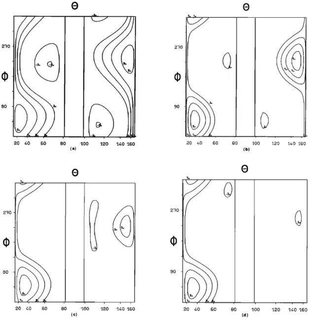
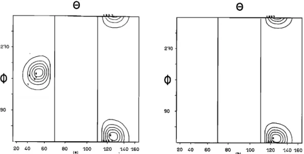
2'•0 2•/0 J • i J j s J , ' i ' i I , 20 40 60 80 '100 '120 '140 '160 20 40 60 80 (c) (d) 100 '120 '1_40 '1_GOFig. 2. Contours
of the averaging
kernel A(cos 6), •; cos 6)o, •o) for 6)o = 30ø and
•o = 30ø. A has been normalized to 10. The scale in amplitude is linear.
There is
a nonpropagating
zone around
6) = •/2 and it is bounded
by leos 6)r = •0/•e with •0 and
•e the wave angular frequency and the electron-angular gyrofrequency. Here •0 =
0.625 kHz, •e = 4. kHz. The electron plasma frequency •e = 18. kHz. We first
consi-
der the magnetic kernels only (N -- 9), then the magnetic and the electric
(N = 36);
M is the number of transformed data we consider. (a) N = 9, M = 5.
(b) N = 9, M = 8.
(c) N = 36, M = ]2. (d) N = 36, M = 16.
M
F(cos
6), (D)=exp
{-1+ Y. pk]ik(COS
6), ½)} (19)
k=l
The new Lagrange multipliers must satisfy the inequality
tp'w'
(2o)
where
6P' is the transformed
error vecto•r,
W' is
the matrix of the measurement
errors in Pk', gi-
ven by W'kL
= <•Pk 6PL >, and z the pr•ecision
with which we intend to fit the M data Pk''
We
practically admit a model error of the same or-der as the errors in the data. Therefore z' is set to M.
The solution of (20) requires that we supply
initial values for the parameters
Pk' Such ini-
tial values can be deduced from a dirichlet ker-nels solution [Lefeuvre
and Delannoy,
1979].
However, we have observed a rapid convergence when starting from a uniform solution, i.e.,
starting will all the Pk equal to zero.
Although the propagation of the instability
is not exactly the same as for the dirichlet kernels solution, the stability and prediction parameters, respectively defined in (]3) and
(]5), have been found to be good quality indi-
2364 Lefeuvre et al.: Geos 1 Wave DistributionsFunctions
vre and Delannoy,
1979]. Obviously,
one must
be very careful in interpreting them. They generally are much more sensitive to an increa- se in M, and we can slightly pass the threshold Q = ! without noting any instability in the solution. This point will be more fully dis- cussed in section 4.
3. Data
The field data are signals obtained by con- tinuous measurements of the electric and magne- tic components of the field. The electric com- ponents are measured by the short axial elec- tric sensors. In the frame of reference of the
satellite they are noted ex, ey, e z. However,
the y component can also be obtained from the long radial antennas. In that case it is noted as E .. The magnetic components are measured atthe •owest
frequencies
(<450 Hz) by the ULF
ma-
gnetic sensors and at other frequencies by the VLF magnetic sensors. To distinguish between
them they are respectively labeled Bx, By, Bz
and b x, by, and b z. For further details see
S-300 Experimenters
[!979].
Because of the incorrect deployment of one of the axial booms, the electric components measu- red onboard Geos ! are not in an orthogonal sys- tem. However, as long as the three electric components are given, there is no difficulty in recalculating them according to the appropriate orthogonal system. This correction is systema- tically done here. The only remaining uncer- tainty is due to the imperfect estimation of the length of the incompletely deployed boom. This uncertainty is negligible relative to the ones we shall encounter later.
Before being transmitted to the ground, the field data are subjected to several onboard treatments, as discussed below.
Six swept frequency analyzers (SFA) process the six components. These analyzers can select a 300-Hz bandwidth in the range 150 Hz-77 kHz, in steps of 300-Hz. The six signals are simul- taneously transposed to the low-frequency range and filtered in the 150- to 450-Hz band. The transposition dephases equally the six signals, so the relative phases stay unchanged. Knowing the transfer function (phase and amplitude) of the filters, one can reconstruct the original wave forms.
Before telemetry, the waveforms are sampled at a rate of ]488 samples per second, which is slightly above the Shannon period. An important drawback of this sampling is that the operations are not simultaneous on the six channels. This time-shift causes a nonnegligible phase-shift, for which a correction must be made.
Between the sensor inputs and the telemetry outputs, there are many opportunities for dis- tortions (sensors, preamplifiers, analyzers, switches, etc.). They globally act as a filter. The transfer function of this equivalent filter is estimated from calibrations made onboard the satellite.
The measurements of electric components are subject to other uncertainties (P.M.E. Decreau, private communication, 1979). The most impor- tant is the one due to the imperfect estimation of the coupling impedance between the plasma and the spheres of the antennas. But it is
also difficult to evaluate the effects of the photocloud and of the thermal sheet around the satellite.
Now the true data, on which we base the esti- mation of the WDF, are the auto and cross-spec- tra of the field components. They are estimated from finite Fourier transforms of the signal. The practical method we use is based on time averaging over short modified periodograms
[Welch,
1967]b
• Let
zi(l) and
z-(l), (! = O,
.... N- 1)
the samples
of t•e components
i
and j, taken in the time interval T, in the frame of reference of the satellite. The re- cords are sectioned in K segments, possibly overlapping, of length L (! = 0 .... L- 1). We consider a Parzen window W(I) and, for each
segment,
form the sequences
[•i(!)W(l)]k,
[zj(l)W(l)]k. We
then take the finite Fourier
transforms of these sequences.
L-1
!
(1)W(1)]kex
p - 2ki!n/L (21)
Ak(n)
= • •Z [z
i
L-l lBk(n)
= • ].=•0
[zJ(l)W(!)]kexp
- 2kiIn/L
and obtain the K modified periodograms
L (n)
B•(n
}
Zk(On
) = U
)
where co = 2vn/L and n L-lI
W
2
u = • z
(•).
]=o (22)The spectral estimate is the average of these periodograms
K
! k
Z Ik(øø
);
Sij(Cøn)
= • =! n
(23)it has a complex value for i • j and a real va- lue for i = j. Such a procedure is well-suited for a multi-component analysis as regards the computer memory which is needed.
We assume that this estimate is unbiased
(<Sij> • Sij) and
that the variance
of the mean
is equal to the variance of the I k divided by
the number
K (var{Re
[S• .] } = K
-• var{Re[I• };
var{Im[.Sij
]} = K
-1 var•m[Ik]}).
The
first
assumptxon tends to be true when the spectra are stationary in frequency, the second when the
number K is large enough and when the I k have a
Gaussian distribution. The two assumptions are more easily fulfilled (which does not mean they are completely fulfilled) for phenomena of the hiss type rather than of the chorus type. Note that the variances calculated are of the same order as the ones estimated from the relations:var {R S.- }
e[ •3]_ TM
Si
iSjj
//•-T where
B is the filter
bandwidth and T is the observation time.
Some operations are required as we attempt to reconstruct from these estimates the spectra of the wave field components. We must correct, as accurately as possible, for the rotation of the satellite (the spin period is of the order of lO rpm) and then for all the distortions intro-
Lefeuvre et al.: Geos 1 Wave Distribution Functions 2365
duced by the electronic and onboard treatment. To minimize the effect of the rotation of the satellite, we consider segments containing a ve- ry low number of samples, typically L = 16, 32, or 64. Between the first and the last samples the rotation is negligible (from 0.6 to 2 de- grees). The resolution in frequency is still reasonable, since it is respectively equal to
46.5, 23.25 or 16.625 Hz.
The following operations are made in this or-
der. The periodograms
Ik(00n) are individually
computed in the frame of reference of their firstpoint.
At each frequency •n, the sampling errors
are corrected by multiplying Ik(C0n) by the factor
exp[•i•n•ij],
the ampies
of the components
where
T
i . is the
i and j.
time
shift
Then the
between
transfer function characterizing the electronic distortions is applied. The periodograms are re- calculated in the frame of reference of the first periodogram (correction for rotation) and avera- ged. Finally the spectral matrix, so obtained, is placed in the Cartesian coordinate system of section 2. The values of the power spectral
densities at the original frequency 00
o are equal
to the values of the power spectral densities at
the frequency •n, the two frequencies being such
that •o = •SFA + •n - 300 Hz with •SFA the cen-
tral frequency of the SFA which is considered.For the sake of simplicity we consider that
the õij s so obtained
ßare unbiased,
and
that the
variances of their real and imaginary parts are the variances, in the appropriate reference sys-
tem, of the estimates defined in (23). This is obviously an optimistic approximation. For a bctter evaluation we should take into account
the errors in our corrections.
As already pointed out there are more uncer- tainties in the electric data than in the magne- tic ones. A way of testing the validity of the electric measurements is to compare the values of the refractive index obtained on the one hand from the plasma parameters measurements and, on
the other hand, from the ratio E/B, assuming
+
that we have whistler mode propagation along B o[Scarf et al., 1969]. In the first case the re-
fractive index, denoted
np, is written
n2 =
e e
P •/•e
(1 - •/• )
e(24)
•e is deduced from the magnetometer data (S331)
and •qe from the wave active experiments (S301 and S304) or by examination of the resonances
of the natural waves. In the second case, the
refractive index, noted nw, can be written (T.
Neubert, private communication, 1979)
n 2 = c2B2/Ef
w(25)
where+
E l is the component
of E perpendicular to
the K vector. An estimate of B 2 is obtainedfrom the magnetic autospectra (c2B 2 = c2D2H
2
= õ44 + õ55 + õ66), and an estimate of E•2øfrom
2=õ
+õ
)
For
the electric
autospectra (Eñ
i i
22 ß
KHz 10 . $ . sx 6 . 4 . 2 . 0 . 10 . 8 . E• 6 . 4 . 2 . 0 . 1t0/1t 20/ 6/19'73 1'7. 0 m 23s(c sc2•.1oo,, i 10 . 8 . sx.E• 6 . 4 _ 2 . 0 .
",o
io
'3o
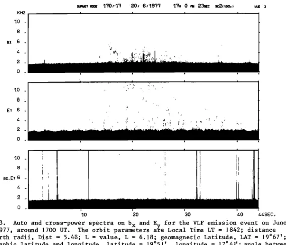
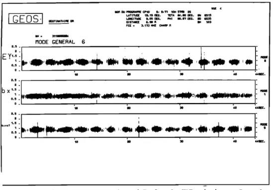
Fig. 3. Auto and cross-power
spectra
on b
x and Ey for the VLF
emission
event on June
20, 1977, around 1700 UT. The orbit parameters are Local Time LT = 1842; distance
in earth radii,
Dist = 5.48; L = value, L = 6.18; geomagnetic Latitude,
LAT = 19ø67';
geogr.
aphlc latitude
and longitude, latitude
= 19 51 , longitude = 17ø41'; angle between
the •o direction and the spin qf the satellite, • = 7ø13
' . The electron
gyrofrequency
estimated from the onboard magnetometer (experiment I S331) is •e = 5.94 kHz. The plas-
2366 Lefeuvre et alo: Geos 1 Wave Distribution Functions
oblique propagation
np and n
w are respectively
low and highe estimates of n.
On 20 cases analyzed up to now, using only the small electric antennas for the electric mea- surements, and at frequencies between 500 Hz and
3 kHz, we have found values of np and n
w such
that 0.5 •< np/n
w •< 1.3, which
indicates relati-
vely good consistency between the electric and magnetic measurements. The agreement seems to be still better when the long radial booms are
used for estimating Ey (T. Neubert, private com-
munication, !979).Other tests could be applied to assess the validity of the electric component. According
to the linearity of equations (2-a), the equali-
ties that exist between
the aij's [Storey
and
Lefeuvre,
1980]
ought
to hold for the õij's at
least in the limit of the errors in the data.
We c•ould expect to have Re(S14) =-Re(S2s);
Im(Szs) = Im(õ24) and Re(õ36) = O. Unfortunate-
ly these equalities are very rarely verified si- multaneously, which limits our expectations for
the electric data. Furthermore, in 'the applica- tions we emphasize the results obtained from the magnetic data.
4. Applications to Geos ! Data Magnetic components. We begin with a detai- led study of a VLF emission that nearly fulfills all the conditions required by the two methods of analysis. Later we shall deal with more dif- ficult cases. As a first step, the analysis is performed with the magnetic data only. The elec- tric data, when available, will be added later.
The first example chosen is a hiss event re-
corded June 20, 1977, around 17OO UT. Its auto
and cross-spectrograms
on b x and Ey are repre-
sented in Figure 3. They have been obtainedfrom the onboard
correlator measurements
[Jones,
1979]. A minor portion of the emission
is avai-
lable at the output of the 3 magnetic SFAs which have a 3OO-Hz bandwidth and sweep the frequency range O-10 kHz in steps of O.69-s duration. The maximum averaged power spectra has been obtained after 17OO. 44 when the SFAs are centered around 600 Hz. We have performed our analysis at530 Hz (for all the sections the resolution fre-
quency is 47 Hz). The phenomenon is fairly stationary in time and frequency. The ratio
00/• e is very small (•O.O9) and one can expect
stable solutions.
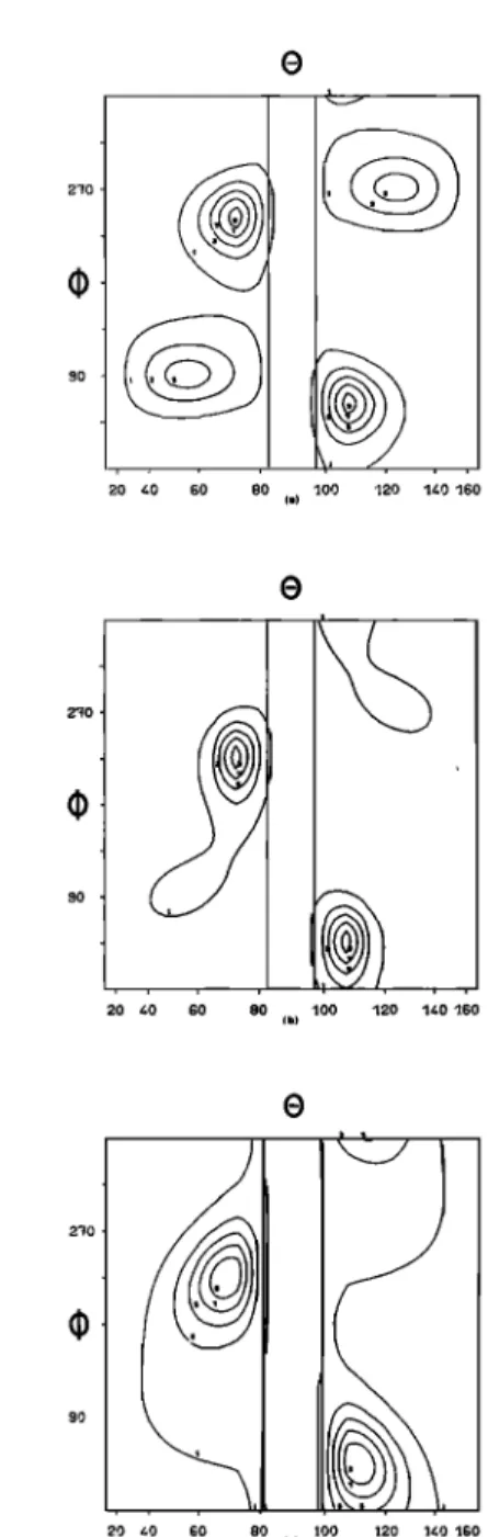
Contours of the dirichlet kernels and maximum entropy solutions are represented in Figure 4 for M = 7, 8• 9. The solutions obtained for M •< 6 appear to be of little value and have not been plotted. Effectively, the first kernels vary roughly in • as sin 2• and cos 2•, and we cannot readily distinguish between solutions at •o and at •o + •'
The dirichlet kernels solutions cannot be ac- cepted as such, in view of the extent of the zo- nes where there are negative values. However, they provide us with useful information. They can effectively be considered as filtered repre- sentations of each possible solution. Although
the transfer function A(cos 0, •; cos 0o, •o) of
the filter presents important side lobes (see
Figure 2 for •o = 30ø and •o = 30ø), we are sure
to determine at least the maximum of the WDF. We cannot be so certain about the interpretation
of the secondary peaks, which might be positive side lobes of the main peak. However, in the present case, because of the amplitudes dis- played, we can expect that there are two maxima of the WDF.
As M varies from 7 to 9, the data Pk are pro-
gressively better fitted. As forecast, the pre- diction parameter reaches the value zero for M = 9. But at the same time, the instability in- creases, and Q goes from O.28 to O.6!. If the solutions for M-- 7 and 8 are quite similar, the one obtained for M = 9 is very different. The peaks have a tendency to appear close to the re- sonance angle, which generally happens in the case of instability. The phenomenon is more no-
ticeable when 00/•
e >• 0.3.
In these cases, Q ta-
kes the values of the order of 2 and more, and
the solution at M = 9 bears no resemblence at all to the ones obtained at M = 7 and M = 8. Finally the solution we select for the hiss event of June 20, 1977, is the one obtained for M = 8 (Figure 4b). It is stable and fits the data well. Its resolving power is superior to the solution for M = 7.
The maximum entropy solutions (Figure 4d, 4e, 4f) are clearly more satisfactory, since they obey the positivity constraint. However, they exhibit the same general features as the dirich- let kernels solutions, which is not surprising considering that the latter can be regarded as filtered representations of any solution and therefore of the maximum entropy solution. A noticeable discrepancy would mean that the so- lution obtained from the maximum entropy method is not a satisfactory solution to our inverse problem, which is theoretically possible since it has never been demonstrated that a maximum entro- py solution always exists. Thus, we can validate the maximum entropy solution by comparing it with the dirichlet kernels solution. This enables us
to interpret the prediction parameter Pr with
much more freedom. A value of Pr reasonably lar-
ger than 1 does not necessarily mean that the ma- ximum entropy solution is invalid. In fact, it generally indicates that there is an inaccurate estimate of the errors on the data.
As for the dirichlet kernels solutions, going from M = 7 to M = 8 we improve the resolving po- wer without changing the main features. At I• = 9
the instability appears to gather all of the energy in the neighborhood of the resonance angle. It is still relatively weak (Q = 1.6) in compari- son with the instability observed in the cases
where
00/•
e >• 0.3 (Q can reach values up to 10
3 )
and for which the initial solutions are complete- ly destroyed. The solution to be selected here is the one obtained at M = 8. Its prediction pa- rameter still has a relatively high value
(Pr = 2.56) but, as was already mentioned, this is not surprising, in view of inaccuracy in the estimation of errors in the data. We could try to improve the fit in taking •' < M in the ine- quality (20). However, we must come to grips with numerical instabilities in the integration of (2').
Finally, the WDF associated with the hiss event of June 20, 1977, is a two-peaked function.
The main peak is centered around • = 60 • (or
120 •) and • = 50 • (or 230•), and the secondary
![Fig. 4. Contours of dirichlet kernels and maximum entropy solutions for 0.69 s of the VLF emission on June 20, ]977, starting around 1700.44 (Figure 3)](https://thumb-eu.123doks.com/thumbv2/123doknet/14797881.604767/11.903.156.787.66.990/contours-dirichlet-kernels-maximum-entropy-solutions-emission-starting.webp)
![Fig. ]3. Averaged wave normal directions. K1 has been systematically taken to indicate the more energetic direction](https://thumb-eu.123doks.com/thumbv2/123doknet/14797881.604767/17.903.126.406.114.513/averaged-normal-directions-systematically-taken-indicate-energetic-direction.webp)
