HAL Id: hal-02369673
https://hal.archives-ouvertes.fr/hal-02369673
Submitted on 19 Nov 2019
HAL is a multi-disciplinary open access
archive for the deposit and dissemination of
sci-entific research documents, whether they are
pub-lished or not. The documents may come from
teaching and research institutions in France or
abroad, or from public or private research centers.
L’archive ouverte pluridisciplinaire HAL, est
destinée au dépôt et à la diffusion de documents
scientifiques de niveau recherche, publiés ou non,
émanant des établissements d’enseignement et de
recherche français ou étrangers, des laboratoires
publics ou privés.
Hugo Larnier, Pascal Sailhac, Aude Chambodut
To cite this version:
Hugo Larnier, Pascal Sailhac, Aude Chambodut. New application of wavelets in magnetotelluric data
processing: reducing impedance bias. Earth Planets and Space, Springer/Terra Scientific Publishing
Company, 2016, 68 (1), �10.1186/s40623-016-0446-9�. �hal-02369673�
LETTER
New application of wavelets
in magnetotelluric data processing: reducing
impedance bias
Hugo Larnier
*†, Pascal Sailhac
†and Aude Chambodut
†Abstract
Magnetotelluric (MT) data consist of the sum of several types of natural sources including transient and quasiperi-odic signals and noise sources (instrumental, anthropogenic) whose nature has to be taken into account in MT data processing. Most processing techniques are based on a Fourier transform of MT time series, and robust statistics at a fixed frequency are used to compute the MT response functions, but only a few take into account the nature of the sources. Moreover, to reduce the influence of noise in the inversion of the response functions, one often sets up another MT station called a remote station. However, even careful setup of this remote station cannot prevent its failure in some cases. Here, we propose the use of the continuous wavelet transform on magnetotelluric time series to reduce the influence of noise even for single site processing. We use two different types of wavelets, Cauchy and Mor-let, according to the shape of observed geomagnetic events. We show that by using wavelet coefficients at clearly identified geomagnetic events, we are able to recover the unbiased response function obtained through robust remote processing algorithms. This makes it possible to process even single station sites and increase the confidence in data interpretation.
Keywords: Magnetotelluric bias, Continuous wavelet transform, Response function, Sferics, Geomagnetic pulsations
© 2016 Larnier et al. This article is distributed under the terms of the Creative Commons Attribution 4.0 International License (http://creativecommons.org/licenses/by/4.0/), which permits unrestricted use, distribution, and reproduction in any medium, provided you give appropriate credit to the original author(s) and the source, provide a link to the Creative Commons license, and indicate if changes were made.
Background
The magnetotelluric (MT) method is based on the induc-tion of natural electromagnetic (EM) fields in the ground. These natural fields can be categorized into two main classes. High-frequency (HF) signals (with frequencies over 1 Hz) are mainly due to lightning activity, and the associated EM waves conveyed in the waveguide made of the ionosphere and the conductive earth. The other main class of EM waves is due to the interaction of the solar wind with the Earth’s magnetic field, and this produces magnetohydrodynamic waves that are transmitted in the atmosphere through the ionosphere from the magneto-sphere (Saito 1969; McPherson 2005).
The MT method is thus based on the quasi-uniform source assumption whereby sources are supposed to be far from the measurement point (Chave and Jones
2012, Chapter 2). In this approximation, the horizontal electric field e = (ex, ey) is linked to the horizontal
mag-netic field h = (hx, hy) by convolution products ∗ (in the
time domain) with impulse response functions (zxx, zxy ,
zyx, and zyy), which are components of the impedance
tensor z:
According to properties of the Fourier transform, this gives us the following relation:
where E and H are the Fourier transform of e and h, respectively, and Zij is a 2 × 2 complex tensor.
(1) ex(t) = zxx(t) ∗ hx(t) + zxy(t) ∗ hy(t), ey(t) = zyx(t) ∗ hx(t) + zyy(t) ∗ hy(t). (2) Ex Ey = Zxx Zxy Zyx Zyy Hx Hy ,
Open Access
*Correspondence: [email protected]†Hugo Larnier, Pascal Sailhac and Aude Chambodut contributed equally
to this work
UMR 7516, Institut de Physique du Globe de Strasbourg, 5 Rue Rene Descartes, 67084 Strasbourg Cedex, France
Z can be transformed into apparent resistivity ρa and
phase φ with:
µ = 4π10−7 H/m being the magnetic permeability, and ω = 2πf with f the signal frequency. These quantities are then analyzed or inverted to infer geoelectrical proper-ties of the subsurface.
Because of the nature of MT time series (e.g., noise heteroscedasticity) and the complexity of the source field (transient nature and diversity of polarizations), Z com-putation is not straightforward. These issues have been the focus of several methods published since the 1970s. Addressing these issues is the objective of this paper.
The first important issue to address is the effect of noise in MT time series. Indeed, Z estimations can be severely down weighted by noise on the magnetic field (Sims et al.
1971). The usual way to get rid of this bias is to set up a second MT station called a remote station (Gamble et al.
1979). This station is used in the processing while assum-ing that sources of noise at both stations are not corre-lated so that the bias is drastically reduced.
The second issue we would like to address comes from the complexity of MT time series that we men-tioned before. The first MT processing techniques (e.g., Sims et al. 1971) were based on least-squares analy-sis which fails in the presence of outliers. Outliers may originate from several issues including non-stationarity, the source effect of MT signals and brief overwhelm-ing noise. Robust statistics were then applied to MT processing to accommodate these outliers (Chave et al.
1987; Egbert and Booker 1986). Another approach was the use of wavelet techniques to look for MT sources or remove noise in the time series. Zhang and Paulson (1997) applied the continuous wavelet transform (CWT) on high-frequency data to select sferics events. They thus increased the signal-to-noise ratio in the response func-tion determinafunc-tion in a straightforward way by the selec-tion of useful signal parts. Trad and Travassos (2000) used wavelets specifically to filter MT data in the time– frequency domain before processing with robust algo-rithms. Escalas et al. (2013) used wavelet analysis to study the polarization properties of cultural noise sources in MT time series.
We took into account the issues of both noise and tran-sient nature of some MT sources by applying the CWT on two types of signals, namely geomagnetic pulsations and sferics. We demonstrate that the CWT may also be a powerful tool to reduce the bias in the computation of the impedance tensor, even in the case of single station processing.
ρa=|Z|2/(µω),
φ = arctan(I(Z)/R(Z)),
Methods
Continuous wavelet transform
The CWT is a mathematical technique used to decom-pose a signal on a time–frequency representation through a special class of functions called wavelets. A wavelet can be defined as a physical event (e.g., Green function) and has to fulfill the following two condi-tions: It has to be localized in both the time and fre-quency domains and has to be a zero-mean function (the so-called admissibility criteria) (Holschneider
1995). The wavelet transform allows one to compute coefficients depending on two factors, the dilatation a >0 (corresponding to frequency) and translation τ (time). Each coefficient is computed following Eq. (3), where s is the analyzed signal (e.g., electric or mag-netic field), ψ is the mother wavelet and ∗ represents
the complex conjugate:
By using the properties of the fast Fourier transform (FFT) with the convolution, one is able to compute wavelet coefficients very quickly.
Wavelet’s choice
In this work, we have chosen two different wavelets, the Cauchy and Morlet wavelets, and each is adapted to the shape of the considered geomagnetic event. Both wavelets are progressive ones with real valued Fourier transform.
The Cauchy wavelet is given in the frequency domain by:
where m is the wavelet’s order (corresponding to the derivative order if an integer), H is the Heaviside step function, Ŵ is the gamma function and a is the dilatation factor.
The Morlet wavelet is given in the frequency domain by:
where ω0 is the central pulsation of the wavelet, H is the
Heaviside function and a is the dilatation factor. Equation (5) does not represent an admissible wavelet if ω0 is not
high enough to fulfill the zero-mean condition. To make it admissible, ω0 must be above π
2/ log(2). A high ω0 implies a high number of oscillations in the wavelet functions.
The following sections illustrate the wavelet choice according to the observed geomagnetic events.
(3) Wψ[s](a, τ ) = +∞ −∞ dt1 aψ ∗ t − τ a s(t) τ ∈ R. (4) ψc(aω) = 2m √ mŴ(2m)H (ω)(aω) me−aω, (5)
ψm(aω) = π−1/4H (ω)e−(aω−ω0)
2/2
Pulsations
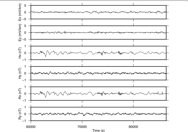
Geomagnetic pulsations are the result of the interac-tions between the solar wind and the magnetosphere, and these events will appear on EM time series as short oscillations (Fig. 1). The pulsations can be divided into two main classes, continuous (Pc pulsations) or irregular (Pi pulsations). Continuous pulsations are quasiperiodic oscillations whose occurrences vary during the day. For example, Pc1 pulsations are predominant during day-hours (in local time) at high latitudes and during night-hours at low latitudes (Saito 1969; Bortnik et al. 2007). Moreover, even during periods of occurence, they often appear as pearls on magnetograms with alternating periods of high and low signal-to-noise ratios (Jun et al.
2014). Irregular pulsations are characterized by a short time duration in comparison with Pc pulsations, and they can be classified as transient events in MT time series. Geomagnetic pulsation signals contain several oscilla-tions so they are very localized in the time and frequency domains simultaneously. Thus, like previous authors (e.g., Zhang and Paulson 1997; Garcia and Jones 2008
for atmospherics signals), we have chosen the Morlet
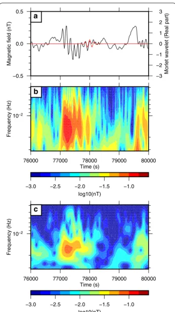
wavelet, which represents the best compromise between the time and frequency resolution. Use of the Cauchy wavelet would be hazardous because of its low-frequency resolution. Both Morlet and Cauchy wavelet coefficients are shown in Fig. 2. As illustrated, the highest coefficients corresponding to the geomagnetic pulsations are much more scattered in terms of the frequency when using then Cauchy wavelet instead of the Morlet wavelet.
Sferics
Sferics are transient events that occur in the frequency band range of 1 Hz to more than 10 kHz (Garcia and Jones 2002). These signals are the most energetic part of the MT signal in these frequency bands (even if other phenomena occur such as Schumann resonances between the waveguide made by the ionosphere and Earth’s surface).
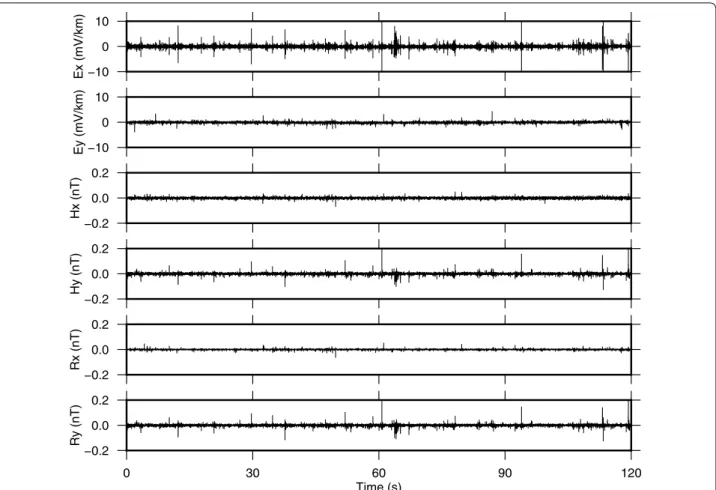
These sferics are characterized by a sudden impulse in the time domain and can be divided into two main frequency bands, namely those above 1 kHz and those below it. In the low-frequency band of extremely low-fre-quency (ELF) waves, sferics consist of a high-amplitude
−5 0 5 Ex (mV/km) −5 0 5 Ey (mV/km) −1 0 1 Hx (nT) −1 0 1 Hy (nT) −1 0 1 Rx (nT) −1 0 1 Ry (nT) 0 0 0 0 8 0 0 0 0 7 0 0 0 0 6 Time (s)
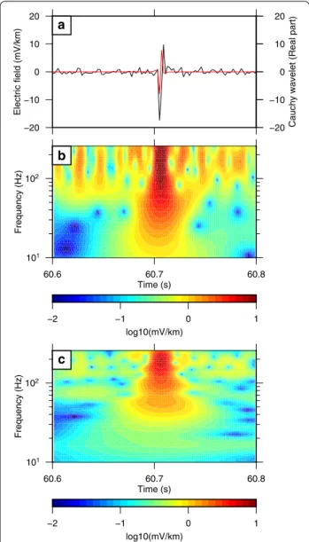
impulse (Fig. 3) called the slow tail (Mackay and Fraser-Smith 2010), whereas in the high-frequency band of very low-frequency (VLF) waves, sferics are mainly shaped as oscillations. To analyze ELF waves using the CWT, we have chosen the Cauchy wavelet. Most of the previous work on MT methods with wavelets was based on the Morlet wavelet stemming from its properties of good res-olution in terms of both the time and frequency (Zhang and Paulson 1997; Garcia and Jones 2008). However, the shape of the ELF wave (Fig. 4a) is very impulsive and
therefore wide in frequency, so it is closer to Cauchy’s shape than to Morlet’s one. Indeed, the ELF wave is very short in time and has very few oscillations, so we need a wavelet that has similar properties. As illustrated in Fig. 4b, c, the highest coefficients obtained with the Mor-let waveMor-let span a wide time length, i.e., longer than the actual length of the ELF wave. Because of their impulsive nature, sferics have a wide frequency content (Mackay and Fraser-Smith 2010). In the time–frequency domain, sferics appear as a series of high-valued coefficients along the frequency axis (very localized in time and spread out in frequency).
Selection of wavelet coefficients
We manually picked geomagnetic events from our MT time series and selected wavelet coefficients from the time–frequency plane by using the following methodology.
In a way similar to wavelet-based denoising techniques, amplitudes of the wavelet coefficients are used to define the selection scheme. The MT system (1) can be solved in a univariate way for ex and ey separately. In both cases,
one has to obtain good signal-to-noise ratios for both hx
and hy. At each scale, for every channel s [output channel
(ex or ey) and input channel (hx, hy)]:
• We compute the median value α of the distribution of |Wψ[s](a, τ )| over a length Ta= Nta around t0 ,
which is the time position of the previously picked event. N in this work is set to 30 and ta is the time
step corresponding to the analyzed scale.
• From this value, we define a threshold set as β times the median value α.
• All coefficients below this threshold level are dis-carded for the magnetotelluric response function computation.
• Coefficients are kept for the final computation when the threshold is reached on (ex, hx, and hy) or (ey, hx,
and hy).
This criterion is sufficient for geomagnetic pulsations (below the Hz). However, for ELF waves, we add one more criteria to fulfill, that is, selected coefficients must span a large frequency range (basically the whole fre-quency range of ELF waves without MT and audio-mag-netotelluric (AMT) dead bands). In practice, we check the Fourier spectrum of the EM time series, which is a good indicator of dead band boundaries. Depending on the signal-to-noise ratio or the time of the day, this limit can be highly variable.
When a remote station is available, we add another criteria to discriminate noise from geomagnetic events. Indeed, the horizontal magnetic coefficients at the
−0.5 0.0 0.5 Magnetic field (nT) −3 −2 −1 0 1 2 3
Morlet wavelet (Real part
) a 10−2 Frequency (Hz) 76000 77000 78000 79000 80000 Time (s) −3.0 −2.5 −2.0 −1.5 −1.0 log10(nT) b 10−2 Frequency (Hz) 76000 77000 78000 79000 80000 Time (s) −3.0 −2.5 −2.0 −1.5 −1.0 log10(nT) c
Fig. 2 Geomagnetic pulsation on Hx and its representation in
time–frequency space. MT site: Piton de la Fournaise (see “Real data application” section). The time axis is the same as Fig. 1. a Comparison between a pulsation (black line) and Morlet wavelet (real part, red
line). b Wavelet coefficients of the pulsation shown in a while using
the Cauchy wavelet. c Wavelet coefficients of the pulsation shown in
remote station have to fulfill the same properties. At the end of this stage, we obtain a group of wavelet coefficients for each scale and each selected geomagnetic event.
Inversion of wavelet coefficients
Zhang and Paulson (1997) demonstrated that Eq. (2) can be written as:
This system of linear equations in the time–frequency domain can be described by the following equation:
where d contains the electric field wavelet coefficients (Wψ[ex](a, τ ), Wψ[ey](a, τ )), G contains the magnetic
field coefficients (Wψ[hx](a, τ ), Wψ[hy](a, τ )) and m
con-tains the MT response functions Z. The classical least-squares solution to this equation is:
(6)
Wψ[ex](a, τ ) = ZxxWψ[hx](a, τ ) + ZxyWψ[hy](a, τ ), Wψ[ey](a, τ ) = ZyxWψ[hx](a, τ ) + ZyyWψ[hy](a, τ ).
(7)
d = Gm,
(8)
Z = (GTG)−1GTd,
This solution is inevitably downward-biased (Sims et al.
1971). One solution is to include a remote station in the processing scheme (Gamble et al. 1979). The solution then becomes:
where Gr contains the remote station magnetic field
coef-ficients Wψ[rx](a, τ ) and Wψ[ry](a, τ ). Another way to
reduce the bias is to actually make the predictor variable (here, the h field) as noise-free as possible. In this alter-nate procedure, our goal is to use the wavelet coefficients of high signal-to-noise ratio geomagnetic events in the computation. By doing so, we will reduce the bias intro-duced by noise on the magnetic field in the solution (8).
To reduce the influence of noise in the electric field, we also use robust statistics instead of classical least squares. As explained in (Chave and Jones 2012 , Chap-ter 5), robust statistics were introduced for MT because of the properties of natural-source electromagnetic data. Among these reasons, they state “finite duration of many geomagnetic or cultural events” and “marked
non-sta-tionarity.” Moreover, the heteroscedasticity of the noise
(9) Z = (GrTG)−1GTrd, −10 0 10 Ex (mV/km) −10 0 10 Ey (mV/km) −0.2 0.0 0.2 Hx (nT) −0.2 0.0 0.2 Hy (nT ) −0.2 0.0 0.2 Rx (nT ) −0.2 0.0 0.2 Ry (nT ) 0 30 60 90 120 Time (s)
Fig. 3 Electromagnetic time series at Rittershoffen MT stations. Sampling frequency: 512 Hz. Time series starts on June 2, 2014, at 18 h 17 min and
can hide natural events along the time series. The main argument for using wavelet transform is precisely to take into account these issues by getting rid of the non-use-ful part of the time series (e.g., no apparent geomagnetic signal) before computing the MT response function. In practice, in many time series the non-useful part is the largest component. Consequently, Z computation is only based on parts of the time series where there is a sig-nificant induction occurring in the subsurface. Indeed, a significant part of the records cannot be used because of the noise level of current state-of-the-art magnetic
sensors (Chave and Jones 2012, Chapter 9). For example, in the AMT dead band, the signal does not rise above the noise level of the induction coils during daytime (Garcia and Jones 2002). Robust statistics are still necessary, but we considerably increase the signal-to-noise ratio on all selected events.
Zhang and Paulson (1997) worked in a single station configuration and used conventional least-squares analy-sis to resolve Eq. (7). Instead of using all selected wave-let coefficients to recover the MT response functions, we estimate the response function on pairs of geomagnetic events. Doing so allows us to build a distribution for each component of the impedance tensor (e.g., Fig. 5).
At each scale for each pair of geomagnetic events, the response function is estimated by using the Huber M-estimator described by Chave et al. (1987) in a MT context. From the distribution of response functions at each scale estimated from all available pairs of geomag-netic events, we represent the final estimation by taking the median value (less sensitive to outliers). The con-fidence interval is represented by using the interquar-tile range (IQR) L-estimator of the distribution (Huber and Ronchetti 2009). The IQR has a breakdown point of 50 %, which makes it robust to long tails in the distribu-tion while still being a good measure of the dispersion or skewness in the distribution.
Real data application Datasets
We applied the previously described technique on two real datasets to illustrate the potential of using
−20 −10 0 10 20 Electric field (mV/km) −20 −10 0 10 20 Cauch y wavelet (Real part) a 101 102 Frequency (Hz) 60.6 60.7 60.8 Time (s) −2 −1 0 1 log10(mV/km) b 101 102 Frequency (Hz) 60.6 60.7 60.8 Time (s) −2 −1 0 1 log10(mV/km) c
Fig. 4 Sferic on Ex and its decomposition in time–frequency space.
MT site: Rittershoffen (see “Real data application” section). Time axis is the same as Fig. 3. a Comparison between a sferic (black line) and Cauchy wavelet (real part, red line). b Wavelet coefficients of the sferic shown in a while using the Cauchy wavelet. c Wavelet coefficients of the sferic shown in a while using the Morlet wavelet
0 10 20 30 40 50 60 Relative frequency (% ) 100 101 102 Apparent resistivity (Ω.m)
Fig. 5 Relative frequency histogram of ρxy at a frequency of 45 Hz.
Processing of Rittershoffen site data using remote reference process-ing. Vertical red thick line: median value of the distribution. Hatched domain: domain defined by the first and third quartile of the distribu-tion
wavelet coefficients on both geomagnetic pulsations and sferics.
The first dataset consists of MT data that were acquired with a sampling frequency of 512 Hz in the northeastern part of France near the town of Rittershoffen as part of a geothermal monitoring experiment (Abdelfettah et al.
2014). The electric measurements were made with EPF06 electrodes and the magnetic measurements with MFS07e coils from Metronix SA. Data in this area are badly con-taminated by 50/3 and 50 Hz noise and their harmonics. We filtered this noise by using a notch filter with 2048 coefficients. The remote used with these measurements is located on the site of the Welschbruch geophysical sta-tion in the Vosges mountains at about 60 km away from the measurement site.
The second dataset consists of electromagnetic hori-zontal measurements that were acquired on the La Four-naise volcano before, during and after the 1998 eruption (Zlotnicki et al. 2005). The data were acquired with a sampling frequency of 0.05 Hz with induction coils simi-lar to those made by Metronix or Phoenix Geophysics (Clerc 1971), and Pb-PbCl2 electrodes. The remote
sta-tion used here is also located on the volcano, a little less than 10 km away from the measurement station.
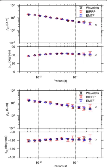
To assess the validity of our method, we have com-pared our results with the ones obtained with robust pro-cessing codes from the work of Alan D. Chave (BIRRP, Bounded Influence Remote Reference Processing, Chave et al. 1987; Chave and Thomson 2004) and Gary Egbert (EMTF, Egbert 1997). For simplicity, we consider error bars as they were calculated by the robust processing codes, even if they can be discussed in more detail (Waw-rzyniak et al. 2013; Chave 2015; Wawrzyniak et al. 2015).
The threshold factor value β was set to 1 for the sferic application and 4 for the pulsation application, but other values can be chosen depending on the signal-to-noise ratio of the processed time series.
Remote processing
We compared the MT response functions obtained by using the wavelet coefficients with those from the appli-cation of other processing codes for both datasets.
In both frequency bands (Figs. 6, 7), the response func-tions obtained with the wavelet coefficients were compa-rable to those obtained with both processing codes. For response functions in the frequency band covered by geomagnetic pulsations (low-frequency band), wavelet inversion was also in agreement with robust process-ing even if the source was not as impulsive as sferics. Figure 5 also demonstrates that the use of robust sta-tistics on the wavelet coefficients of only two events allowed for the recovery of the response functions with good accuracy.
Single site processing
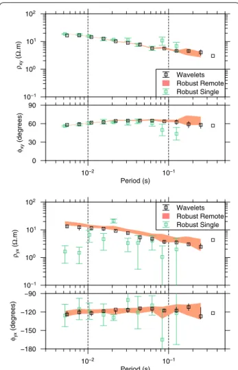
For single site processing, we processed single site MT stations by removing the remote station for all process-ing codes. For visual comparison, only BIRRP results are shown, but conclusions remain the same for EMTF.
For high-frequency results (Fig. 8), ρyx was
downward-biased by noise over a large frequency bandwidth and ρxy was also biased around 0.08 Hz. Because of the
posi-tion of the staposi-tion near housing, it was difficult to assess where the noise source was (it could have been from elec-tric fences or pipelines). In this case, the result given by robust processing in the single site configuration would lead to a wrong interpretation of the MT response. Wavelet processing allows one to drastically reduce the noise bias and recover the impedance tensor obtained by using remote processing even near the 50 Hz frequency.
For low-frequency processing (Fig. 9), the single site ρxy was slightly downward-biased by noise where the
10−1 100 101 102 ρxy (Ω .m ) 0 30 60 90 φxy (degrees) 10−2 10−1 Period (s) 10−1 100 101 102 ρyx (Ω .m) −180 −150 −120 −90 φyx (degrees) 10−2 10−1 Period (s) Wavelets BIRRP EMTF Wavelets BIRRP EMTF
Fig. 6 Comparison of wavelet-based determination of the
imped-ance tensor and robust algorithms. MT site: Rittershoffen site with remote reference processing
wavelet-based result remained within the confidence bounds of the remote processing. Particularly, the ρxy
component was very sensitive to the coherence param-eter. Some examples of interpretable MT responses for this component are illustrated in Fig. 10. If the coherence parameter is too low (below 0.5), ρxy is distinctly biased
by noise (up to a factor of three) for periods below 200 s.
Other transient applications
So far, we have illustrated only two types of transient sig-nals, namely sferics in their lowest frequency range (e.g., slow tails) and geomagnetic pulsations. This approach can also be applied on wider MT bands than the ones presented in this paper.
For higher-frequency applications, the slow tails stud-ied in this paper already contain frequency content above 256 Hz (up to 1 kHz). Other impulsive waves such as VLF
waves have a distinctive signature in the time–frequency plane and frequency content from 1 kHz up to more than 10 kHz (Rakov and Uman 2003). In Fig. 11, we show an example of such a VLF wave and its time–frequency analysis. These waves were already used in an MT pro-cessing study by Zhang and Paulson (1997).
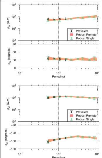
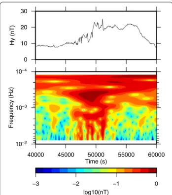
The assortment of low-frequency geomagnetic sources is large. Among transient events at periods lower than 200 s, there are Pc5 geomagnetic pulsations that have periods up to 500–600 s (Saito 1969). Geomagnetic storms are also low-frequency sources of induction. They have already been studied with wavelet analysis (e.g., Mendes et al. 2005). We show, for example, in Fig. 12 a signal of interest at low frequency that was recorded on the Piton de La Fournaise volcano on July 16, 1997, and the signal contains significant frequency content up to more than 1000 s. 100 101 102 103 ρxy (Ω .m) 0 30 60 90 φxy (degrees) 101 102 103 Period (s) 100 101 102 103 ρyx (Ω .m ) −180 −150 −120 −90 φyx (degrees) 101 102 103 Period (s) Wavelets BIRRP EMTF Wavelets BIRRP EMTF
Fig. 7 Comparison of wavelet-based determination of the
imped-ance tensor and robust algorithms. MT site: Piton de la Fournaise site with remote reference processing
10−1 100 101 102 ρxy (Ω .m) 0 30 60 90 φxy (degrees) 10−2 10−1 Period (s) 10−1 100 101 102 ρyx (Ω .m) −180 −150 −120 −90 φyx (degrees) 10−2 10−1 Period (s) Wavelets Robust Remote Robust Single Wavelets Robust Remote Robust Single
Fig. 8 Comparison of wavelet-based determination of the
imped-ance tensor and robust algorithms. MT site: Rittershoffen site in single site processing
Conclusion
We have shown through these experiments that the con-tinuous wavelet transform (CWT) is an easy and efficient way to characterize the magnetotelluric (MT) response function for transient geomagnetic events. Using this technique, we have shown that most of the informa-tion contained in the source wavelet coefficients is suf-ficient in datasets to enable the characterization of the MT impedance tensor. Two types of geomagnetic events were studied, geomagnetic pulsations and sferics, and thus this work increases the frequency band studied in previous publications involving CWT application during MT processing. The mother wavelet has to be adapted to each transient event to accurately recover the source
100 101 102 103 ρxy (Ω .m) 0 30 60 90 φxy (degrees) 101 102 103 Period (s) 100 101 102 103 ρyx (Ω .m ) −180 −150 −120 −90 φyx (degrees) 101 102 103 Period (s) Wavelets Robust Remote Robust Single Wavelets Robust Remote Robust Single
Fig. 9 Comparison of wavelet-based determination of the
imped-ance tensor and robust algorithms. MT site: Piton de la Fournaise site in single site processing
101 102 103 Apparent resistivity ρ (Ω .m) 101 102 103 Period (s) Remote reference results:
BIRRP with remote station data Single site results:
Wavelet based results
BIRRP using a 0.5 coherence threshold BIRRP using a 0.7 coherence threshold BIRRP using a 0.9 coherence threshold Fig. 10 Dependance of ρxy robust results on the coherence
param-eter. MT site: Piton de la Fournaise site in single site processing
−0.4 −0.2 0.0 0.2 0.4 Hx (nT) 103 104 Frequency (Hz) 0.300 0.305 0.310 Time (s) −3 −2 −1 log10(nT)
Fig. 11 Very low-frequency wave in the Hx time series at
information. Even irregular geomagnetic pulsations that are very localized in the time and frequency domains simultaneously can be used in MT processing. The other transient sources of induction are currently being investi-gated and will be the subject of future papers on wavelet analysis of magnetotelluric time series.
We have also shown that we were able to drastically reduce the noise bias of the considered datasets on the MT response function in the case of a single station con-figuration. This was achieved by using the high signal-to-noise ratio transient events in the MT time series. By using robust statistics with only two geomagnetic events in the wavelet domain, we were able to recover accurate response functions.
Yet, we still have to develop a way to automatically detect geomagnetic events to analyze their properties (e.g., polarization) and their effect on MT impedance computation.
Author’s contributions
The manuscript was written by HL and reviewed by all authors. All authors read and approved the final manuscript.
Acknowledgements
We would like to thank the three anonymous reviewers who greatly helped to improve this manuscript. We thank the LABEX G-Eau-Thermie of the University of Strasbourg and the field crew (Y. Abdelfettah) for the acquisition of MT measurements at Rittershoffen. We also thank J. Zlotnicki for Le Piton de la
Fournaise EM time series. Finally, we also acknowledge discussions with vari-ous colleagues and students at early stages of this work.
Competing interests
The authors declare that they have no competing interests. Received: 3 December 2015 Accepted: 14 April 2016
References
Abdelfettah Y, Sailhac P, Schill E, Larnier H (2014) Preliminary magnetotelluric monitoring results at Rittershoffen. In: 3rd European geothermal work-shop, Karlsruhe, 15–16 Oct 2014
Bortnik J, Cutler JW, Dunson C, Bleier TE (2007) An automatic wave detection algorithm applied to Pc1 pulsations. J Geophys Res 112:A04204. doi:10.1 029/2006JA011900
Chave A (2015) Comment on “Robust error on magnetotelluric impedance estimates” by P. Wawrzyniak, P. Sailhac and G. Marquis. Geophys Prospect.
doi:10.1111/j.13652478.2012.01094.x
Chave AD, Jones A (2012) The magnetotelluric method: theory and practice. Cambridge University Press, Cambridge
Chave AD, Thomson DJ (2004) Bounded influence magnetotelluric response function estimation. Geophys J Int 157(3):988–1006
Chave AD, Thomson DJ, Ander ME (1987) On the robust estimation of power spectra, coherences, and transfer functions. J Geophys Res 92(B1):633–648
Clerc G (1971) Contribution à l’optimisation des capteurs à induction destinés à la mesure des variation du champ magnétique terrestre (10−3 à 104 Hz).
PhD thesis, Paris, France
Egbert GD (1997) Robust multiple-station magnetotelluric data processing. Geophys J Int 130(2):475–496
Egbert GD, Booker JR (1986) Robust estimation of geomagnetic transfer func-tions. Geophys J R Astron Soc 87(1):173–174
Escalas M, Queralt P, Ledo J, Marcuello A (2013) Polarisation analysis of magnetotelluric time series using a wavelet-based scheme: a method for detection and characterisation of cultural noise sources. Phys Earth Planet Interiors 218:31–50
Gamble TD, Goubau WM, Clarke J (1979) Magnetotellurics with a remote magnetic reference. Geophysics 44(1):53–68
Garcia X, Jones AG (2002) Atmospheric sources for audio-magnetotelluric (AMT) sounding. Geophysics 67(2):448–458
Garcia X, Jones AG (2008) Robust processing of magnetotelluric data in the AMT dead band using the continuous wavelet transform. Geophysics 73(6):223–234
Holschneider M (1995) Wavelets: an analysis tool. Oxford Science Publications, Oxford
Huber PJ, Ronchetti EM (2009) Robust statistics, 2nd edn. Wiley, New York Jun C, Shiokawa K, Connors M, Schofield I, Poddelsky I, Shevtsov B (2014)
Study of Pc1 pearl structures observed at multi-point ground stations in Russia, Japan, and Canada. Earth Planets Space 66(140):1–14
Mackay C, Fraser-Smith AC (2010) Lightning location using the slow tails of sferics. Radio Sci 45(5). doi:10.1029/2010RS004405
McPherson RL (2005) Magnetic pulsations: their sources and relation to solar wind and geomagnetic activity. Surv Geophys 26(5):545–592
Mendes O Jr, Domingues MO, da Costa M, Clúa de Gonzalez A (2005) Wavelet analysis applied to magnetograms: singularity detections related to geomagnetic storms. J Atmos Solar Terr Phys 67:1827–1836
Rakov VA, Uman MA (2003) Lightning: physics and effects. Cambridge Univer-sity Press, Cambridge
Saito T (1969) Geomagnetic pulsations. Space Sci Rev 10:319–412 Sims WE, Bostick FXJ, Smith HW (1971) The estimation of
magnetotel-luric impedance tensor elements from measured data. Geophysics 36(5):938–942
Trad DO, Travassos JM (2000) Wavelet filtering of magnetotelluric data. Geo-physics 65(2):482–491
Wawrzyniak P, Sailhac P, Marquis G (2013) Robust error on magnetotelluric impedance estimates. Geophys Prospect 61:533–546
0 10 20 30 Hy (nT) 10−4 10−3 10−2 Frequency (Hz) 40000 45000 50000 55000 60000 Time (s) −3 −2 −1 0 log10(nT)
Fig. 12 Low-frequency variations of the magnetic field at the Piton
Wawrzyniak P, Sailhac P, Marquis G (2015) Reply of the authors to AD Chave’s comment on Wawrzyniak P., Sailhac P. and Marquis G. 2013. Robust error on magnetotelluric impedance estimates. Geophys Prospect 64(1):250–251
Zhang Y, Paulson KV (1997) Enhancement of signal-to-noise ratio in natural-source transient magnetotelluric data with wavelet transform. Pure Appl Geophys 149:405–419
Zlotnicki J, Le Mouël J-L, Gvishiani A, Agayan S, Mikhailov V, Bogoutdinov S, Kanwar R, Yvetot P (2005) Automatic fuzzy-logic recognition of anoma-lous activity on long geophysical records: application to electric signals associated with the volcanic activity of La Fournaise volcano (Reunion Island). Earth Planet Sci Lett 234:261–278