HAL Id: hal-01268909
https://hal.archives-ouvertes.fr/hal-01268909
Submitted on 28 May 2020
HAL is a multi-disciplinary open access
archive for the deposit and dissemination of
sci-entific research documents, whether they are
pub-lished or not. The documents may come from
teaching and research institutions in France or
abroad, or from public or private research centers.
L’archive ouverte pluridisciplinaire HAL, est
destinée au dépôt et à la diffusion de documents
scientifiques de niveau recherche, publiés ou non,
émanant des établissements d’enseignement et de
recherche français ou étrangers, des laboratoires
publics ou privés.
observations: benefit of Monte Carlo versus variational
schemes and analyses of the year-to-year model
performances
Diego Santaren, Philippe Peylin, Cédric Bacour, Philippe Ciais, Bernard
Longdoz
To cite this version:
Diego Santaren, Philippe Peylin, Cédric Bacour, Philippe Ciais, Bernard Longdoz. Ecosystem model
optimization using in situ flux observations: benefit of Monte Carlo versus variational schemes and
analyses of the year-to-year model performances. Biogeosciences, European Geosciences Union, 2014,
11 (24), pp.7137-7158. �10.5194/bg-11-7137-2014�. �hal-01268909�
www.biogeosciences.net/11/7137/2014/ doi:10.5194/bg-11-7137-2014
© Author(s) 2014. CC Attribution 3.0 License.
Ecosystem model optimization using in situ flux observations:
benefit of Monte Carlo versus variational schemes and
analyses of the year-to-year model performances
D. Santaren1,2, P. Peylin2, C. Bacour3, P. Ciais2, and B. Longdoz4
1Environmental Physics, Institute of Biogeochemistry and Pollutant Dynamics, ETH Zurich, Universitätstrasse 16, 8092 Zurich, Switzerland
2Laboratoire des Sciences du Climat et de l’Environnement, Commissariat à l’Energie Atomique, L’Orme des Merisiers, 91190 Gif sur Yvette, France
3NOVELTIS, 153, rue du Lac, 31670 Labège, France
4INRA, UMR 1137, Ecologie et Ecophysiologie Forestires, Centre de Nancy, 54280 Champenoux, France
Correspondence to: D. Santaren (jean-diego.santaren@env.ethz.ch)
Received: 23 October 2013 – Published in Biogeosciences Discuss.: 20 November 2013 Revised: 28 October 2014 – Accepted: 7 November 2014 – Published: 16 December 2014
Abstract. Terrestrial ecosystem models can provide major insights into the responses of Earth’s ecosystems to envi-ronmental changes and rising levels of atmospheric CO2. To achieve this goal, biosphere models need mechanistic formu-lations of the processes that drive the ecosystem functioning from diurnal to decadal timescales. However, the subsequent complexity of model equations is associated with unknown or poorly calibrated parameters that limit the accuracy of long-term simulations of carbon or water fluxes and their in-terannual variations. In this study, we develop a data assimi-lation framework to constrain the parameters of a mechanis-tic land surface model (ORCHIDEE) with eddy-covariance observations of CO2and latent heat fluxes made during the years 2001–2004 at the temperate beech forest site of Hesse, in eastern France.
As a first technical issue, we show that for a complex process-based model such as ORCHIDEE with many (28) parameters to be retrieved, a Monte Carlo approach (genetic algorithm, GA) provides more reliable optimal parameter values than a gradient-based minimization algorithm (vari-ational scheme). The GA allows the global minimum to be found more efficiently, whilst the variational scheme often provides values relative to local minima.
The ORCHIDEE model is then optimized for each year, and for the whole 2001–2004 period. We first find that a re-duced (< 10) set of parameters can be tightly constrained by the eddy-covariance observations, with a typical error reduc-tion of 90 %. We then show that including contrasted weather regimes (dry in 2003 and wet in 2002) is necessary to opti-mize a few specific parameters (like the temperature depen-dence of the photosynthetic activity).
Furthermore, we find that parameters inverted from 4 years of flux measurements are successful at enhancing the model fit to the data on several timescales (from monthly to interan-nual), resulting in a typical modeling efficiency of 92 % over the 2001–2004 period (Nash–Sutcliffe coefficient). This sug-gests that ORCHIDEE is able robustly to predict, after opti-mization, the fluxes of CO2and the latent heat of a specific temperate beech forest (Hesse site). Finally, it is shown that using only 1 year of data does not produce robust enough optimized parameter sets in order to simulate properly the year-to-year flux variability. This emphasizes the need to as-similate data over several years, including contrasted weather regimes, to improve the simulated flux interannual variabil-ity.
1 Introduction
In the context of global warming and climate change, the in-teractions between the terrestrial biosphere and the climate system play a crucial role (Field CB, 2004). Particularly, it is of fundamental importance to assess precisely the distri-bution and future evolution of terrestrial CO2 sources and sinks and their controlling mechanisms. To understand and predict CO2, water and energy exchanges between the veg-etation and atmosphere, process-driven land surface mod-els (LSMs) provide insights into the coupling and feedbacks of those fluxes with changes in climate, atmospheric com-position and management practices. To achieve this goal, LSMs need finely to describe the processes (i.e., photosyn-thesis, respiration, evapotranspiration, etc.) that regulate the exchanges between the biosphere and the atmosphere across a wide range of climate and vegetation types and timescales. The level of complexity of LSMs usually encapsulates a de-scription of processes whose timescales range from hours to centuries and whose spatial coverage can spread from flux tower footprints to the global scale.
The equations and parameters of LSMs are usually de-rived from limited observations on the leaf, soil unit, or plant scales, and are limited to a few plant species, climate regimes, or soil types. Because of the spatial heterogeneity of ecosystems and the nonlinear relationship between parame-ters and fluxes, difficulties arise in upscaling small-scale pro-cess parametrizations and formulations to larger scales, from canopies to ecosystems, regions, and global scales (Field et al., 1995). As a result, major uncertainties remain in mod-eling the future and global responses of the terrestrial bio-sphere to changes in the climate and CO2 (Friedlingstein et al., 2006; Denman et al., 2007).
By fusing observations to model structures, data assim-ilation methods have shown large potential for improving and constraining biogeochemical models (Wang et al., 2001; Braswell et al., 2005; Trudinger et al., 2007; Santaren et al., 2007; Wang et al., 2009; Williams et al., 2009; Kuppel et al., 2012). Particularly, the time-series measurements from the FLUXNET network provide valuable information on ex-changes of CO2, water and energy across a large range of ecosystems and timescales (Baldocchi et al., 2001; Williams et al., 2009; Wang et al., 2011). At each site out of the 500 sites of this network, fluxes are measured with the eddy-covariance method (Aubinet et al., 1999) on a half-hourly basis and for observation periods that can reach more than 10 years.
Some previous works focused on quantifying how much information could be retrieved from the observations in terms of reducing uncertainties in model parameters. The ap-proach relied on the minimization of a cost function with re-spect to model parameters. Wang et al. (2001) showed that about three or four parameters of a rather simplified terres-trial model could be estimated independently by assimilating 3 weeks of eddy-covariance measurements of CO2 and
la-tent, sensible and ground heat fluxes. Braswell et al. (2005) used a 10 year record of half-hourly observations of CO2flux to study the influence of data frequencies on inverted param-eters. It was shown that parameters related to processes op-erating on diurnal and seasonal scales (evapotranspiration, photosynthesis) were tightly constrained compared to those related to processes with longer timescales. Santaren et al. (2007) conducted a similar study, but used a complex mech-anistic model (ORCHIDEE) with more than 15 parameters to be optimized. In that study, the data assimilation framework was also employed to highlight model structural deficiencies and to improve process understanding.
Performances of parameter optimization schemes have been investigated in several studies (Richardson and Hollinger, 2005; Trudinger et al., 2007; Lasslop et al., 2008; Fox et al., 2009; Ziehn et al., 2012). They could be strongly affected by the way observation errors are prescribed within misfit functions (Richardson and Hollinger, 2005; Trudinger et al., 2007; Lasslop et al., 2008). Contrarily, the choice of the minimizing method amongst an exhaustive panel (locally gradient-based or global random search methods, Kalman filtering) was shown to have smaller influences (Trudinger et al., 2007; Fox et al., 2009; Ziehn et al., 2012). Recently, Ziehn et al. (2012) optimized a simplified version of the process-based BETHY model against atmospheric CO2 ob-servations. They demonstrated that a gradient-based method (variational approach) manages to locate the global mini-mum of their inverse problem similarly to a Monte Carlo approach based on a metropolis algorithm, but with compu-tational times several orders of magnitude lower.
Carvalhais et al. (2008) challenged the commonly made assumption of carbon cycle steady state at ecosystem level for parameter retrieval, and proposed to optimize parameters describing the distance from equilibrium of soil carbon and biomass carbon pools. More recently, data assimilation im-plementations have been tested in terms of error propaga-tion, i.e., how information retrieved on optimized parameters influences carbon flux estimation on various timescales (Fox et al., 2009). In those studies, models with a moderate level of complexity were used, and a limited number of parameters was optimized, typically less than 10.
Several studies have shown that calibrating models on a certain timescale does not necessarily imply that predic-tive skills are improved on all timescales (Hui et al., 2003; Siqueira et al., 2006; Richardson et al., 2007). Particularly, it is important to assess whether the forecast capability of the model could be dampened because of model shortcomings in simulating interannual or long-term processes. One im-portant test of prognostic ability is to assess the model skills in simulating the interannual variability (IAV) of ecosystem carbon fluxes (Hui et al., 2003; Richardson et al., 2007).
The fact that the FLUXNET observations provide infor-mation from hourly to interannual timescales allows the in-vestigation of potential time dependencies of parameters, thus highlighting missing processes that should be included
in the models on specific timescales. Reichstein (2003) found that for a rather simple photosynthetic model applied to Mediterranean summer dry ecosystems, parameters should vary seasonally to match observed CO2 and water fluxes. Similarly, Wang et al. (2007) showed that, for deciduous forests, the photosynthetic parameterization of their model should integrate seasonal variations related to leaf phenol-ogy in order to obtain realistic patterns of CO2, water and energy fluxes. More recently, and in order to search for re-lationships between carbon fluxes and climate, Groenendijk et al. (2009) optimized a simple vegetation model with only five parameters and investigated the weekly variability of in-verted values with respect to different climate regions and vegetation types. Few studies have specifically investigated the equations and parameter generalities across time and spa-tial scales of complex process-based models. Kuppel et al. (2012) analyzed the ability of a process-based terrestrial bio-sphere model (ORCHIDEE) to reproduce carbon and water fluxes across an ensemble of FLUXNET sites corresponding to a particular ecosystem (temperate deciduous broadleaf for-est), but left apart a detailed study of the model performances across temporal scales.
In this work, we use the same ORCHIDEE model, but we focus on the temporal scale and study the temporal skill of the equations in reproducing seasonal and year-to-year CO2and water flux variations at a particular deciduous for-est site. To tackle this scientific qufor-estion, we also invfor-estigate in a preliminary step the potential of two different optimiza-tion approaches, comparing a gradient-based scheme and a Monte Carlo (genetic algorithm) scheme, to infer the opti-mal parameters of the process-based model. We use eddy-covariance measurements (daily mean of CO2and latent heat fluxes) in a beech forest in France (Hesse) for 4 years (2001– 2004) characterized by different weather regimes. More specifically, we investigate the following questions:
– How does a gradient-based method perform compared to a more systematic search of the optimal parameters based on a genetic algorithm (GA)?
– Does the assimilation of 1 year or 4 years of data en-hance the model fit to observations equally?
– Are the model equations generic enough to simu-late seasonal and year-to-year variations of the CO2 and water fluxes, and particularly the extreme years (e.g., the summer drought of 2003)?
– Does the information gained from parameter optimiza-tion indicate anything new about modeling carbon and water fluxes in deciduous forests?
After a description of the methods (Sect. 2), performances of the gradient-based and GA algorithms are compared (Sect. 3.1). We then optimize the model with daily means of eddy-covariance NEE and water fluxes observed at the
Hesse tower site over the 2001–2004 period. Through cross-validation experiments, we assess the predictive skills of the model when optimized with each different year and with the whole period of data (Sect. 3.2). A posteriori parame-ter values, errors and correlations are analyzed in order to quantify the contribution of the data assimilation framework in terms of parameter calibration and process understand-ing (Sect. 3.3). Particularly, we investigate to what extent optimized values may have been biased to compensate for model structural deficiencies. Finally, the temporal skill of the model is studied through its ability to reproduce vari-ations in the NEE from monthly to interannual timescales (Sect. 4.3).
2 Material and methods 2.1 Eddy-covariance flux data
The beech forest of Hesse is located in northeastern France (48◦N, 7◦E). It is a fenced experimental plot where many studies have been carried out (see the references in Granier et al., 2008). In 2005, it was a nearly homogeneous plan-tation of 40 year old European beech (Fagus sylvatica L.) whose mean height was 16.2 m. Located on a high-fertility site, this young forest, which underwent thinning in 1995, 1999 and at the end of 2004, is growing relatively quickly, and thus acts on an annual basis as a net carbon sink (aver-age NEE equals −550 g C m−2yr−1over 2001–2004). Long-term mean annual values of temperature and rainfall are, re-spectively, 8.8◦C and 900 mm.
Fluxes and meteorology are measured in situ and on a 30-min basis by using the standardized CARBO-EUROFLUX protocol (Aubinet et al., 1999). We use hereinafter observa-tions that were made at the HESSE site from 2001 to 2004. Within this period, less than 5 % of the net CO2flux (NEE) and latent heat flux (LE) data were missing, and observa-tional gaps mostly occurred during December 2001, Febru-ary and December 2004, where periods with no data lasted around 10 days. We use original data that were neither cor-rected for low-turbulence conditions, nor gap filled, nor par-titioned (Reichstein et al., 2005; Papale et al., 2006). Data corrections only accounted for inner canopy CO2storage.
NEE and to a lesser extent LE fluxes showed high year-to-year variability related to soil water deficit duration and growing season length (Granier et al., 2008). Years 2001 and 2002 were, respectively, moderately dry and wet, whereas 2003 and 2004 were exceptionally dry (respectively, 124 and 100 days of soil water deficit). Moreover, during the summer of 2003 (June to August), mean monthly temperatures were the highest ever observed in this area. Finally, the growing season length (GSL) varied significantly during this period, with an amplitude of 50 days, mostly because of different senescence dates.
2.2 The ORCHIDEE land surface model
The ORCHIDEE (ORganizing Carbon and Hydrology In Dynamic Ecosystems) biogeochemical ecosystem model is a mechanistic land surface model that simulates the exchanges of carbon dioxide, water and heat fluxes within the soil– vegetation system and with the atmosphere; variations in wa-ter and carbon pools are predicted variables. Model processes are computed on a wide range of timescales: from 30 min (e.g., photosynthesis, evapotranspiration, etc.) to thousands of years (e.g., passive soil carbon pool decomposition) (Krin-ner et al., 2005). ORCHIDEE has been applied in a number of site-level (Krinner et al., 2005) and regional CO2 budget studies forced by climate data (Jung et al., 2007), as well as for future projections of the carbon–climate system, coupled to an atmospheric model (Cadule et al., 2010).
The model contains a biophysical module dealing with photosynthesis and energy balance calculations every 30 min, a carbon dynamics module dealing with the alloca-tion of assimilates, autotrophic respiraalloca-tion components, on-set and senescence of foliar development, mortality and soil organic matter decomposition in a daily time step. A com-plete description of ORCHIDEE can be found in Krinner et al. (2005). The main parameters optimized in this study are defined in Table 1, and the associated model equations are defined in Appendix A. The choice of a subset list amongst the total number of ORCHIDEE parameters is explained in Sect. 2.3.4.
As in most land surface models (LSMs) dealing with bio-geochemical processes, the vegetation is described in OR-CHIDEE by plant functional types (PFT), with 13 different PFT over the globe. Distinct PFT follow the same set of gov-erning equations, but with different parameter values, except for the calculation of the growing season onset and termi-nation (phenology), which involves PFT-specific equations (Botta et al., 2000). The Hesse forest is described here by a single PFT called “temperate deciduous”, in the absence of understory vegetation at the forest site. Soil fractions of sand, loam and clay are 0.08, 0.698 and 0.222, respectively (Quentin et al., 2001).
In the following, we applied the model in a “grid-point” mode, forced by 30 min gap-filled meteorological measure-ments made on the top of the flux tower (Krinner et al., 2005). Forcing variables are air temperature, rainfall and snowfall rates, air-specific humidity, wind speed, pressure, and short-wave and longshort-wave incoming radiations.
Biomass and soil carbon pools are initialized to steady-state equilibrium from a spin-up run of the model, i.e., a 5000 year model run using climate forcing data from years 2001 to 2004 repeated in a cyclical way. This ensures an annual net carbon flux close to zero in a multi-year aver-age period. This strong assumption is partly released through the optimization of a scaling factor of the soil carbon pools (Ksoil C, Eq. A17) to match the observed carbon sink
asso-ciated with this growing forest (see Sect. 4.2 and Carvalhais et al., 2008).
2.3 Parameter optimization procedure
The methodology that we use in this study to optimize the ORCHIDEE parameters relies on a Bayesian framework (Tarantola, 1987): (1) we select a set of parameters to opti-mize, and a range of variation for each parameter; (2) assum-ing Gaussian probability density functions (PDF) to describe data and parameter distributions, we define a cost function that embodies a measure of the data–model misfit and prior information on the parameters; (3) we test the performances of a genetic algorithm and a gradient-based one to minimize the cost function, i.e., to locate the optimal parameter set within the parameter space; and (4) we assess errors and cor-relations in optimized parameters.
2.3.1 Cost function
Assuming that the probability density functions of the er-rors in measurement, model structure and model parameters are Gaussian, the optimal parameters correspond to the min-imum of the cost function J (x) (Tarantola, 1987):
J (x) = (Y − M(x))tR−1(Y − M(x)) + (x − xp)tB−1(x − xp) (1)
x is the vector of parameters to be optimized, xpthe vector of prior parameter values, Y is the vector of observations, and M(x) the vector of model outputs. The error covariance matrices R and B describe the prior variances/covariances in observations and parameters, respectively. The first term of J (x) represents the weighted data–model squared devi-ations (referred to in the text below as JOBS, Sect. 3.2.1). The second term, which is inherent to Bayesian approaches, represents the mismatch between optimized and prior values weighted by the prior uncertainties in parameters (diagonal matrix B, Table 1). Although we acknowledge that obser-vation and parameter errors do not strictly follow Gaussian distributions, we have used such a hypothesis to simplify the Bayesian optimization problem, which becomes equivalent to a least squares minimization and thus analytically solv-able by minimizing a cost function like Eq. (1) (Tarantola, 1987).
The temporal resolution of M(x) and Y corresponds to daily averages. We choose daily means in order to assess the ability of the ORCHIDEE model to reproduce observed CO2 and latent heat flux variability on daily, weekly, seasonal, and interannual timescales, and not the hourly timescale. Because of data gaps, daily means have been calculated only when more than 80 % of the half-hourly data were available.
R, the data error covariance matrix, should include both data uncertainties (diagonal elements) and their correlations (non-diagonal elements). However, the latter are difficult to assess properly, and we thus neglect them. Data uncertainties (R diagonal elements) are chosen in such a way that NEE and
Table 1. Parameter names with their description and corresponding model equations (Appendix A), ranges of variation, a priori values and
uncertainties of the parameters.
Parameter Description Prior Min Max σprior
Photosynthesis
Vcmax_opt Maximum carboxylation rate (µmol m−2s−1) (Eq. A5) 55 27 110 33.2
gsslope Slope of the Ball–Berry relationship between assimilation and
stomatal conductance (Eq. A2)
9 0 12 4.8
cTopt Optimal temperature for photosynthesis (◦C) (Eq. A11) 26 6 46 16
cTmin Minimal critical temperature for photosynthesis (◦C) (Eq. A9) −2 −7 3 4
cTmax Maximal critical temperature for photosynthesis (◦C) (Eq. A10) 38 18 58 16
Stomatal response to water availability
Fstressh Adjust the soil water content threshold beyond which stomata
close because of hydric stress (Eq. A6).
6 0.8 10 3.7
Kwroot Root profile that determines the soil water availability (Eq. A7) 0.8 0.2 3 1.12
Phenology
Kpheno_crit Parameter controlling the start of the growing season (Eq. A30) 1 0.5 2 0.6
cTsen Temperature parameter controlling the start of senescence
(Eq. A33)
12 2 22 8
LAIMAX Maximum leaf area index (Eqs. A32 and A31) 5 3 7 1.6
SLA Specific leaf area (Eq. A28) 0.026 0.013 0.05 0.015
Lage_crit Mean critical leaf lifetime (Eq. A34) 180 80 280 80
KLAIhappy Multiplicative factor of LAIMAX that determines the
thresh-old value of LAI below which the carbohydrate reserve is used (Eq. A32)
0.5 0.35 0.7 0.14
τleafinit Time in days to attain the initial foliage using the carbohydrate
reserve (Eq. A31)
10 5 30 10
Respirations
KsoilC Multiplicative factor of the litter and soil carbon pools
(Eq. A17)
1 0.25 4 1.5
Q10 Parameter driving the exponential dependency of the
het-erotrophic respiration on temperature (Eq. A18)
2 1 3 0.8
MRoffset Offset of the linear relationship between temperature and
main-tenance respiration (Eqs. A15 and A14)
1 0.1 2 0.76
MRslope Slope of the linear relationship between temperature and
main-tenance respiration (Eqs. A15 and A14))
0.16 0.05 0.48 0.172
KGR Fraction of biomass allocated to growth respiration (Eq. A16) 0.28 0.1 0.5 0.16
Respirations responses on water availability
HRHa Parameter of the quadratic function determining the moisture
control of the heterotrophic resp. (Eq. A20)
−1.1 −2 0 0.8
HRHb Parameter of the quadratic function determining the moisture
control of the heterotrophic resp. (Eq. A20)
2.4 1.8 6 1.7
HRHc Parameter of the quadratic function determining the moisture
control of the heterotrophic resp. (Eq. A20)
−0.3 −1 0.5 0.6
HRHmin Minimum value of the moisture control factor of the
het-erotrophic respiration (Eq. A20)
0.25 0.1 0.6 0.2
Zdecomp Scaling depth (m) that determines the effect of soil water on
litter decomposition (Eqs. A19 and A21)
0.2 0.05 5 2
Zcrit_litter Scaling depth (m) that determines the litter humidity (Eq. A22) 0.08 0.01 0.5 0.2
Energy balance
Kz0 Rugosity length scaling the aerodynamic resistance of the
tur-bulent transport (Eq. A13)
0.0625 0.02 0.1 0.03
Kalbedo_veg Multiplicative parameter of vegetation albedo (Eq. A23) 1 0.8 1.2 0.16
Table 2. Data errors that are taken into account within the cost
func-tion (matrix R, Eq. 1). They were determined as the RMSE between a priori model outputs and observations (see text).
Years 2001 2002 2003 2004 2001–
2004 (4Y) NEE (gC m−2day−1) 2 2.5 1.7 1.6 1.9
LE (W m−2) 14 12 26.3 20.5 19
LE observations have similar weights in the inversion pro-cess; they are defined as the root mean squared error (RMSE) between the prior model and the observations (Table 2). This rather simple formulation leads to relatively large errors (typ-ically 25 % of the maximal amplitude of daily fluxes), which reflects the fact that data uncertainties comprise not only the measurement errors (random and systematic), but also signif-icant model errors (representativeness issues as well as miss-ing processes).
The magnitudes of prior parameter uncertainties (matrix B) were chosen (i) according to expert knowledge and (ii) to be relatively large, to minimize the influence of the Bayesian term and thus to provide the maximum leverage of the ob-servations upon the parameters. Moreover, for the minimiza-tion algorithms, an addiminimiza-tional important informaminimiza-tion is the range of variation for each parameter; such range is pre-scribed from expert knowledge and typical observed values (TRY database: http://www.try-db.org). As in Kuppel et al. (2012), the prior error for each parameter was thus set to 40 % of its prescribed range of variation (Table 1) and we do not consider correlations between a priori parameter values. 2.3.2 Minimization algorithms
Gradient-based algorithm. Several numerical algorithms can
be used to minimize a cost function (Press et al., 1992; Trudinger et al., 2007). In this article, we tested two ap-proaches. The first one, the L-BFGS-B algorithm (Byrd et al., 1995), belongs to the family of gradient-based methods that follow local gradients of the cost function to reach its mini-mum. It was specifically designed for solving nonlinear op-timization problems with the possibility of accounting for bounds on the parameters. The algorithm requires at each it-eration the value and the gradient of the cost function with respect to its parameters.
The computation of the gradient can be done straightfor-wardly and precisely by using the tangent linear model (TL). For complex models, the construction of the TL model is a rather sophisticated operation (even with automatic dif-ferentiation tools (Giering et al., 2005)) where threshold-based formulations are not handled and need to be rewritten with sigmoid functions for instance. Alternatively, gradients computations can be approximated with a finite-difference scheme. In this study, we use the TL model of ORCHIDEE, generated by the automatic differentiator tool TAF
(Gier-ing et al., 2005). The computation of the gradient of J with respect to one parameter requires one run of the TL model whose computing cost is about two times a standard run of ORCHIDEE. As the L-BFGS-B algorithm requires around 40 iterations to converge (termination criterion: rel-ative change of the cost function does not exceed 10−4 dur-ing five iterations) and as we optimize a set of 28 parameters, the total computing time of an optimization is close to 2400 model runs.
Even though the derivatives of J (x) are estimated pre-cisely by the use of TL models, the main drawback of the gradient-based algorithms is that they may end up on lo-cal minima instead of locating the global minimum. To as-sess the importance of this problem, optimizations from dif-ferent initial parameter guesses have been performed (see Sect. 3.1).
Genetic algorithm. Our second approach to minimizing J
is based on a genetic algorithm (GA) that operates a stochas-tic search over the entire parameter space. The GA was cho-sen from other global search algorithms (simulated anneal-ing, Monte Carlo Markov chains (MCMC)) because of its ease of implementation and its efficiency in terms of con-vergence. Particularly, MCMC algorithms were discarded given that their computational expense may be prohibitive with global terrestrial ecosystem models (Ziehn et al., 2012). The GA mimics the principles of genetics and natural selec-tion (Goldberg, 1989; Haupt and Haupt, 2004). When ap-plying a GA for an optimization problem, parameter vectors are considered as chromosomes whose each gene represents a parameter. Every chromosome chr has an associated cost function J (chr) (Eq. 1), which assigns a relative merit to that chromosome. The algorithm starts with the definition of an initial population of nchr chromosomes; each parameter value being randomly chosen within a defined interval (Ta-ble 1). Cost functions are then computed for each chromo-some. Then, the GA follows a sequence of basic operations to create a new population: (1) Selection of chromosomes from the current population (parents) that will (2) mate and form new chromosomes (children) by exchanging part of their genes (crossover). (3) Additionally, some new chromo-somes will come from the mutation of some parents chro-mosomes. This mutation induces random changes in the pa-rameters (genes) of the parents leading to new chromosomes that are partly independent of the current population. Finally, depending on the user choice, a new generation can be cre-ated in several ways: (1) by gathering the current and new populations; (2) by selecting the best chromosomes, i.e., the ones that have the lowest cost function, amongst both pop-ulations (elitism); and (3) by integrating the new population only. This new generation is used in the next iteration of the algorithm.
GA performances are sensitive to the way their processes are implemented (selection, recombination or mating, muta-tion) and to the values of their principal parameters: num-ber of chromosomes nchr, fraction of chromosomes that mate
or mutate, and number of iterations. The best configuration should provide a good balance between, on the one hand, ro-bustness and precision, and, on the other hand, rapidity. In our study, we tested different configurations by optimizing the model against the 2001 Hesse data. The chosen setup of the GA leads on average to the smallest optimal cost function with the smallest number of iterations. For this configuration, the population is of 30 chromosomes and the maximal num-ber of iterations is set to 40. The total computing cost of the GA is hence about 1200 model runs (versus the 2400 model runs of the gradient-based algorithm). Moreover, we set that 80 % of the children chromosomes are created by reproduc-tion processes, and 20 % by mutareproduc-tions. The chromosomes are selected for mating by a roulette wheel process over their cost function values (Goldberg, 1989) and, once two chromo-somes have been selected for recombination, they exchange their genes (parameters) by a double crossover point scheme (Haupt and Haupt, 2004). Next generations are then created by selecting the 30 best chromosomes amongst the parents and the children (elitism). This ensures that the population size will be constant.
2.3.3 Posterior uncertainty assessment
Once the minimum of the cost function has been reached by one or the other algorithm – i.e., optimal parameter values have been found – it is crucial to determine which param-eters, through the data assimilation system, have been best resolved and which ones have not. Posterior errors and cor-relations in optimized parameters provide not only an answer to this question, but also the sensitivities of the cost function to each parameter.
If the model is linear with Gaussian distributions for data and initial parameter errors, the posterior probability distri-bution of the optimized parameters is also Gaussian (Taran-tola, 1987). The posterior error covariance matrix Pacan be
directly computed as Pa= [Ht∞R
−1H
∞+B−1]−1. (2)
The matrix H∞ represents the derivative of all model
out-puts with respect to parameters at the minimum of the cost function. Square roots of diagonal terms of Paare parameter
uncertainties. Large absolute values (close to 1) of correla-tions derived from Pa indicate that the observations do not
provide independent information to separate a given pair of parameters (Tarantola, 1987).
2.3.4 Optimization settings: parameters to be optimized?
To simplify the problem, we first select among all OR-CHIDEE parameters the most significant ones that primar-ily drive, from synoptic to seasonal timescales, NEE and LE variations. Accordingly, we do not consider, for example, the optimization of soil carbon turnover or tree growth
parame-ters that impact the NEE mainly on decadal scales. Finally, we choose a subset of 28 parameters controlling photosyn-thesis, respirations, phenology, soil water stresses and energy balance (Table 1).
Although only few parameters may be constrained by the observations of NEE and LE, we optimize a large ensemble because it is difficult to assess beforehand parameter sensi-tivities over the whole parameter space. One drawback may be that the algorithm would give spurious optimized values because of the equifinality problem whereby multiple com-binations of parameters yield similar fits to the data (Med-lyn et al., 2005; Williams et al., 2009). The analysis of the posterior error covariance matrix (Pa, Eq. 2) will inform on
which parameters are reliably constrained by the observa-tions (Sect. 3.1).
3 Results
3.1 Performances of a gradient-based versus Monte Carlo minimization algorithm
To assess the relative performances of the BFGS and GA al-gorithms, we designed a twin experiment, using outputs of the model as synthetic data. This model simulation was done for year 2001 with parameters values that were randomly chosen within their permitted range of variation (Table 1). This artificial data set is fully consistent with the model and therefore the optimization of the parameters is not biased by potential model deficiencies or by observations uncertainties. The objective is to assess the accuracy of the optimization al-gorithms by comparing the assimilated parameters with the “true” ones used to create the synthetic data. Consequently, in order to let the optimization freely recover these parame-ters, we remove the term of the cost function that restores optimized values to the prior parameter estimates (Eq. 1). We then ran 10 twin optimizations with each algorithm. For the BFGS approach, we started the downhill iterative search from 10 different initial parameters sets that were randomly prescribed within the admissible range of variation of the parameters (Table 1). For the GA, each optimization gives different results, as several of the GA major operations are based on a random generator.
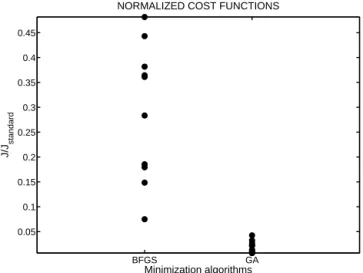
To compare the a posteriori cost functions, we choose to normalize their values by the value of the cost function ob-tained by running the ORCHIDEE model with its standard parameters. GA shows a much more robust behavior than BFGS insofar as the normalized cost function values for that algorithm range from 0.007 to 0.04 (mean value 0.02, stan-dard deviation 0.01, Fig. 1). In comparison, the BFGS al-gorithm produces a posteriori cost functions between 0.07 and 0.49 (mean value 0.29, standard deviation 0.14; Fig. 1). Given the complexity of the ORCHIDEE model, the cost function is likely characterized by multiple local minima. These twin experiments thus clearly show that the GA is
BFGS GA 0.05 0.1 0.15 0.2 0.25 0.3 0.35 0.4 0.45
NORMALIZED COST FUNCTIONS
Minimization algorithms
J/J
standard
Figure 1. Cost function reductions for the 10 twin experiments
that were performed with the BFGS algorithm (BFGS) and with the genetic algorithm (GA). Cost functions (J ) at the end of the minimization process were normalized by the value of the cost function representing the mismatch between the synthetic data and the model outputs computed with the standard parameters of OR-CHIDEE (Jstandard).
probably more efficient in minimizing complex cost func-tions than the BFGS, which is prone, depending on the ini-tial parameter guesses, to falling into local minima. Note that, for our problem, the computing cost of the GA (1200 model runs) is also lower than for the BFGS (2400 model runs).
On average, none of the two algorithms worked well in re-trieving the “true” parameter values that were used to gener-ate the synthetic data (Fig. 2). For the best realization of each algorithm, the mean retrieval score across parameters (based on the ratio of the estimated and true values) is about 1, but with a standard deviation of 35 %. Both algorithms likely fail to overcome the equifinality problem; the chosen data ilation framework and more specifically the type of assim-ilated data (NEE and LE daily means) do not allow one to distinguish parameters that are correlated (see Sect. 4.2). For most parameters, however, the true values lie in the uncer-tainty range of the optimized values (1 sigma of the Gaussian PDF), with the error bars crossing the unit horizontal line. Those inverted parameters that show large differences from their a priori values are also characterized by large errors. As Santaren et al. (2007) illustrated for the ORCHIDEE model, the more uncertain an optimized parameter is, the more likely the possibility that the equifinality problem could affect this parameter.
The retrieved parameters that are far from the truth are as-sociated with large posterior error correlations with other pa-rameters, which may explain poor inversion skills. For ex-ample, the BFGS optimization did not manage to determine accurately the parameters cTopt, cTmax, Q10, KGR, HRHa, HRHb, HRHc and Krsoil. Figure 3 shows that the errors on
these parameters are strongly correlated with each others. Besides, these correlations are consistent with the model structure as they concern parameters that are involved in the simulation of the same processes. For instance, HRHa, HRHb and HRHc define the soil humidity control of the heterotrophic respiration (Eq. A20). In summary, we stress again the need to use the information from the posterior variance–covariance matrix, and especially the correlations between parameter errors, to highlight the level of constraint on each parametrization (see Sect. 3.3 with real data). 3.2 Temporal skill of the model equations
The twin experiment results have shown that the genetic al-gorithm is a more robust method than the gradient-based BFGS algorithm in optimizing the parameters of a model with the complexity of ORCHIDEE. Therefore, we use the GA algorithm to fuse the model with real data collected at the Hesse site.
To address the issue of the temporal skill of the model equations, i.e., their ability to represent year-to-year flux variations, we have designed five cross-validation experi-ments where the ORCHIDEE parameters are optimized us-ing the Hesse data for different years: 2001, 2002, 2003, and 2004, and for the whole period (2001–2004). The corre-sponding optimized parameter sets are called X2001, X2002, . . . , X4Y. Then, for every five optimized parameter sets, we successively run the model forward and examine the fits to the observations over each year and over 2001–2004. The model runs with X2001, X2002, . . . and X4Y are, respectively, called ORC2001, ORC2002, . . . , ORC4Y. As expected, the pa-rameter set inverted from observations of a given time period leads to the best model–data agreement during that time pe-riod.
Through cross-validation experiments, we investigate how parameters optimized with 1 year or the whole period of ob-servations affect the simulations. More precisely, the opti-mization against 4 years of observations allows one to es-timate if the equations are generic enough to simulate the year-to-year flux variations. Using the 1 year optimized pa-rameter sets to simulate the other years helps to assess the benefit of multi-year versus single-year optimizations. Note that the range of weather conditions during the period 2001– 2004 was large, with the wet period in 2001–2002 and the dryer conditions in 2003–2004. This contrast strengthens the analysis of the temporal skill of the model equations. 3.2.1 Cost function reductions
Overall optimization efficiency. For a given time period of
assimilated data, the total data–model misfit produced by the resulting optimal parameters is dramatically reduced with re-spect to the prior one (Fig. 4a). Across the different time peri-ods, the term of the cost function representing the total data– model misfit (JOBS, Eq. 1) is divided by 1 order of magnitude
Figure 2. Twin experiments results in terms of parameter inversion. For each parameter, the retrieved values (x) corresponding to the best
realization of each minimization algorithm (Min. algo.: BFGS, GA) are divided by the true values (xtrue) that were used to generate the data
so that a value of 1 indicates a perfect retrieval (horizontal lines within the boxes). Along with these values are the a posteriori uncertainties normalized to the true parameter values.
(mean ratio ≈ 0.09, blue line Fig. 4a) with a standard devia-tion of 0.04. The different years show different ratios ranging from 0.05 (2002) to 0.14 (2001–2004). These results show that the data assimilation framework has fulfilled its primary target of reducing the total misfit between model outputs and observations. Besides, even though the minimization of the total cost function (Eq. 1) does not make any distinction be-tween types of data, the partial cost functions JNEEand JLE
have been reduced by similar amplitudes, respectively, by 88 % and 93 %, with a standard deviation of 4 % for both (green and red lines, Fig. 4a).
Performances of the 4 year optimized parameter set. The
2001–2004 data inversion leads on average to a significant improvement of the fit to the data for each single year of the 2001–2004 period (mean JOBS reduction ≈ 0.16, Fig. 4f)). Even better, the dispersion from year to year of the JOBS
re-ductions is relatively small (≈ 0.04). Hence, the single pa-rameter set X4Y not only enhances the global fit to the 2001– 2004 data, but also leads to a significant improvement in the simulation of each single year. These results indicate a sub-stantial predictive ability of the model for periods including wet and very dry summers such as in 2003.
Performances of the 1 year optimized parameter sets. The
Xiparameters appear not to be generic enough to enhance in
the same proportions the model fit to data of a different year
j than the year i of the optimization (j 6= i). When using the 1 year inverted parameters to simulate data of a differ-ent year, the JOBS cost functions are decreased on average by 68.5 % (mean ratio post/prior JOBS: 0.22 for X2001, 0.4 for X2002, 0.31 for X2003 and 0.33 for X2004; blue line in Figs. 4b, c, d, e). In comparison, these parameters lead on the year used for their optimization to a mean reduction of
Figure 3. A posteriori correlations between the optimized
param-eters corresponding to the best twin BFGS optimization. Red and blue squares are, respectively, related to pairs of parameters that are strongly correlated and anticorrelated. White cells correspond to correlations whose absolute values are lower than 0.1.
92 % (ratio post/prior JOBS: 0.13 for X2001on 2001, 0.05 for
X2002on 2002, 0.06 for X2003 on 2003 and 0.07 for X2004 on 2004; Fig. 4a). Likely, the data assimilation framework does not extract enough information from 1 year of data to retrieve robust parameters for simulations in different years. This is particularly true because we have different weather regimes during summer, very dry and hot in 2003 and 2004, normal in 2001 and wet in 2002. The 1 year optimized pa-rameters sets tend to produce reasonable fits for years with similar climates, but much poorer fits for the other years. Over the whole 2001–2004 period, the JOBS reductions are about 79 %, 67 %, 76 % and 75 % for X2001, X2002, X2003 and X2004, respectively (mean reduction ≈ 74 %), which is slightly lower that the reduction for the X4Y parameter set (86 %, Fig. 4f).
3.2.2 Fit to the observations
The above analysis of cost function reductions has provided a general and quantitative overview of the performances of the optimized models. Results are now discussed in terms of seasonal fits to NEE and LE.
NEE prior model–data disagreement. The prior model
overestimates the magnitude of ecosystem respiration in win-ter for all years (green curves, Fig. 5). As noticed in Sect. 2.2, carbon pools were initialized from a steady-state spin-up run and the modeled NEE does not represent the current forest carbon uptake (mean NEE = −550 g C m−2yr−1). Also, the prior model does not fully capture the magnitude of the sum-mer uptake period from July to August. ORCHIDEE with prior parameters is however able to reproduce the effect of
2001 2002 2003 2004 4Y 0 0.1 0.2 0.3 0.4 0.5 0.6 Optimization performances a) Inverted time−period
Ratio opt/prior cost function
2001 2002 2003 2004 4Y 0 0.1 0.2 0.3 0.4 0.5 0.6 b) Parameter set: X2001 Time−period
Ratio opt/prior cost function
2001 2002 2003 2004 4Y 0 0.1 0.2 0.3 0.4 0.5 0.6 c) Parameter set: X2002 Time−period
Ratio opt/prior cost function
2001 2002 2003 2004 4Y 0 0.1 0.2 0.3 0.4 0.5 0.6 d) Parameter set: X 2003 Time−period
Ratio opt/prior cost function
2001 2002 2003 2004 4Y 0 0.1 0.2 0.3 0.4 0.5 0.6 e) Parameter set: X 2004 Time−period
Ratio opt/prior cost function
2001 2002 2003 2004 4Y 0 0.1 0.2 0.3 0.4 0.5 0.6 f) Parameter set: X 4Y Time−period
Ratio opt/prior cost function
Figure 4. (a) Cost function reductions after optimization of the
model against observations of each time period (2001, 2002, . . . , 4Y for the whole 2001–2004 time period). Blue bars are associated with the term of the cost function representing the total data–model misfit (JOBS, Eq. (1)); green and red bars are associated with partial
cost functions relative to NEE and LE data, respectively (JNEEand
JLE). The horizontal lines represent the mean values of the
corre-sponding cost functions reductions. Figures (b), (c), . . . , (f) show the cost function reductions produced when running the model with the corresponding optimized parameter sets (X2001, . . . , X4Y) in
every time period. Horizontal lines are the averaged cost function reductions across other years than the one used to optimize the model.
the strong summer 2003 drought, which causes a positive NEE anomaly (Fig. 5c). Finally, the prior model is unsuc-cessful in reproducing the beginning and the end of the car-bon uptake season during most years but 2003: the starting and finishing dates are on average earlier than 13 days com-pared to reality.
NEE optimization efficiency. The optimization
success-fully corrects most of the mismatches described above. For each year, the amplitudes of observed winter release and summer uptake are properly simulated by the model run with the parameter set inverted from that year of observations. The beginning and the end of the carbon uptake seasons are also correctly determined compared to the prior model: after opti-mization, the mean delay between the model outputs and the observations is decreased to 2.5 days and 2.75 days for the starting and finishing dates, respectively.
Seasonal cycle of the carbon uptake. The 4 year inverted
parameter set X4Y leads to a correct simulation of the phase and amplitude of the seasonal cycle of the carbon uptake for most of the years (Figs. 5a, b, c, d). On the contrary, the model run with 1 year optimized parameter sets tends to reproduce the start of the NEE decrease during spring of a different year more incorrectly than the one used for the inversion. A good example of this bias is the model run with X2003, which predicts a NEE decrease much earlier than
Figure 5. For 2001, 2002, 2003 and 2004, fits to the net CO2flux
observations (thick black curve) of the model run with the prior and the optimized parameter sets. Figure legends show the model– data RMSE for the different parameter sets. Observation errors are represented by the grey shaded area.
observed for the years 2001, 2002 and 2004 (Figs. 5a, b, d). Probably, the description of leaf onset processes (Botta et al., 2000) is too empirical to allow capturing of year-to-year vari-ations when its associated parameters (Kpheno_crit, KLAIhappy and τleafinit) are optimized with only 1 year of data. Moreover, 1 year optimized models fail to simulate the observed carbon uptake magnitude of a different year. For instance, the model parameterized with X2001, X2003and X2004systematically underestimates the carbon uptake amplitude of the year 2002 (Fig. 5b).
Extreme 2003 summer drought. None of the optimized
models but ORC2003was able to reproduce the amplitude of the abnormally low uptake during September 2003 (Fig. 5c). Most of them (ORC2001, ORC2004 and ORC4Y) reproduce efficiently the effect of the hydric stress and the subsequent sharp drop in CO2uptake at the beginning of August, during heat wave conditions, but they overestimate the follow-up re-covery of NEE in September. Detailed in situ measurements
Figure 6. For 2001, 2002, 2003 and 2004, fits to the latent heat flux
observations (thick black curve) of the model run with the standard and the optimized parameter sets. Figure legends show the model– data RMSE for the different parameter sets. Observation errors are represented by the grey shaded area.
have led to the conclusion that heavy hydric stress events may damage photosynthetic organs, inhibiting further photosyn-thetic assimilation, or may cause embolism due to cavitation (Breda et al., 2006). As these physiological behaviors are not modeled by ORCHIDEE, most of the inverted models, ex-cept ORC2003, consistently overestimate the gross primary production (GPP) during September 2003. To fit NEE 2003 data, the optimization probably produces misleading values of the X2003parameters (notably cTmax; see Sect. 3.3), which in turn explains the poor NEE fit during September 2001, 2002 and 2004 of the ORC2003model.
LE prior model disagreement with data. For all years, the
prior model overestimates the magnitude of the latent heat flux nearly all year long (Figs. 6a–d). This bias is particu-larly important during summertime periods, and dry years such as 2003 and 2004. The LE bias reaches up to 40 W m−2 in 2003–2004 compared to 20 W m−2in 2001–2002. In ad-dition, prior modeled LE may precede the observation in
2001 2002 2003 2004 4Y 30 40 50 60 70 80 90 100 110 Vcmax_opt 2001 2002 2003 2004 4Y 4 6 8 10 12 14 gsslope 2001 2002 2003 2004 4Y 10 15 20 25 30 35 40 45 cTopt 2001 2002 2003 2004 4Y −6 −4 −2 0 2 cTmin 2001 2002 2003 2004 4Y 20 25 30 35 40 45 50 55 cTmax 2001 2002 2003 2004 4Y 1 2 3 4 5 6 7 8 9 10 Fstressh 2001 2002 2003 2004 4Y 0.5 1 1.5 2 2.5 3 Kwroot 2001 2002 2003 2004 4Y 0.5 1 1.5 2 Kpheno_crit 2001 2002 2003 2004 4Y 5 10 15 20 cTsen 2001 2002 2003 2004 4Y 3 3.5 4 4.5 5 5.5 6 6.5 7 LAIMAX 2001 2002 2003 2004 4Y 0.015 0.02 0.025 0.03 0.035 0.04 0.045 0.05 SLA 2001 2002 2003 2004 4Y 100 150 200 250 Lage_crit 2001 2002 2003 2004 4Y 0.35 0.4 0.45 0.5 0.55 0.6 0.65 KLAIhappy 2001 2002 2003 2004 4Y 5 10 15 20 25 30 τleafinit 2001 2002 2003 2004 4Y 0.5 1 1.5 2 2.5 3 3.5 4 KsoilC 2001 2002 2003 2004 4Y 1 1.5 2 2.5 3 Q10 2001 2002 2003 2004 4Y 0.1 0.15 0.2 0.25 0.3 0.35 0.4 0.45 0.5 KGR 2001 2002 2003 2004 4Y 0.2 0.4 0.6 0.8 1 1.2 1.4 1.6 1.8 MRoffset 2001 2002 2003 2004 4Y 0.05 0.1 0.15 0.2 0.25 0.3 0.35 0.4 0.45 MRslope 2001 2002 2003 2004 4Y −2 −1.5 −1 −0.5 0 HRHa 2001 2002 2003 2004 4Y 2 2.5 3 3.5 4 4.5 5 5.5 6 HRHb 2001 2002 2003 2004 4Y −1 −0.5 0 0.5 HRHc 2001 2002 2003 2004 4Y 0.1 0.2 0.3 0.4 0.5 0.6 HRHmin 2001 2002 2003 2004 4Y 0.5 1 1.5 2 2.5 3 3.5 4 4.5 5 Zdecomp 2001 2002 2003 2004 4Y 0.05 0.1 0.15 0.2 0.25 0.3 0.35 0.4 0.45 Zcrit_litter 2001 2002 2003 2004 4Y 0.02 0.03 0.04 0.05 0.06 0.07 0.08 0.09 0.1 Kz0 2001 2002 2003 2004 4Y 0.8 0.85 0.9 0.95 1 1.05 1.1 1.15 Kalbedo_veg 2001 2002 2003 2004 4Y 2 4 6 8 10 12 14 x 104 Krsoil
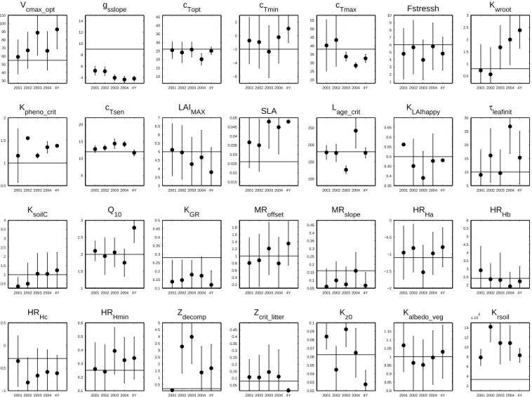
Figure 7. Optimized parameter values (circles) and errors (vertical bars) estimated by the data assimilation system in every time period
(2001, 2002, . . . , 4Y for 2001–2004). Box heights specify the ranges within parameters are allowed to vary during the optimization process. Horizontal lines are the a priori values of the parameters.
spring. This phase difference is particularly striking in 2002 and 2004, when canopy evapotranspiration starts much ear-lier than observed. This could be related to biased param-eterization of leafout phenological processes or to a wrong assessment of the transpiration intensity. Also, observations of LE may be underestimated because of the lack of energy closure observed in FLUXNET data (Wilson et al., 2002).
LE optimization efficiency. For each 1 year parameter
in-version, the corresponding optimized model reproduces sub-stantially better the LE observations than the prior model for that particular year (Figs. 6a–d). Nevertheless, for each year but 2002, it underestimates both the peak of LE in early June and the subsequent decrease of the transpiration over the summer (Figs. 6a, c and d). Possibly, these deficiencies illus-trate structural shortcomings of the model in correctly com-puting the stomatal conductance and/or the vapor pressure deficit during summer periods, with a “big leaf” approach
(Jarvis P.G., 1995) that does not consider any gradient of hu-midity from the free atmosphere down to the leaf level.
LE fits of the 4 year optimized model versus the 1 year op-timized models. As expected, the inversion using the whole
period (X4Y parameters) produces the best compromise throughout the years. Indeed, for a given year of obser-vations, ORC4Y generally outperforms the models inverted from a different year, with the two exceptions of the fits to the LE data of 2002 by ORC2001and 2004 by ORC2003. 3.3 Parameter and uncertainty estimates
Level of constraint on the parameters. Only a few
param-eters are tightly constrained by the observations if we take as a criterion an error reduction greater than 90 % (error reduction ≡ ratio of the a posteriori uncertainty to the range of variation). The optimized values of these parame-ters are characterized by lower relative a posteriori uncertain-ties than other parameters (Fig. 7). When inverting 4 years
30 60 90 120 150 180 210 240 270 300 330 360 −700 −600 −500 −400 −300 −200 −100 0 100 200 NEE (gC/m 2/yr) DOY
Figure 8. Yearly trend of the cumulative weekly NEE averaged over
2001–2004 for the observations (black curve), for the model run with the a priori parameter set (green curve) and with the 2001– 2004 inverted parameter set (X4Y, blue curve).
of observations, nine parameters are determined precisely by the optimization framework: gsslope (stomatal conductance, Eq. A2), cTopt (temperature control of the photosynthesis, Eq. A11), cTmax(temperature control of the photosynthesis, Eq. A10), Kpheno_crit (leaf onset, Eq. A30), cTsen (tempera-ture control of the senescence, Eq. A33), SLA (specific leaf area, Eq. A28), Lage_crit(leaf age driving of the senescence, Eq. A34), KLAIhappy(leaf onset, Eq. A32) and Zcrit_litter(litter humidity, Eq. A22). The inversion of 1 year of observations produces a lower constraint on the parameters: only four, three, five and five parameters are precisely determined for the 2001, 2002, 2003 and 2004 optimizations, respectively. Whatever the time period used for the optimization, 18 pa-rameters are weakly constrained by the observations. Note that, contrary to previous studies, the maximum photosyn-thetic carboxylation rate (Vcmax_opt, Eq. A5) is not among the most constrained parameters (Wang et al., 2001, 2007; Santaren et al., 2007).
Hydric stress constraints. The data assimilation
frame-work optimizes processes related to the temperature control of the carbon assimilation to match the observed NEE dur-ing hydric stress events. The cTmax parameter (Eq. A10), the maximal temperature where photosynthesis is possible, is indeed much better constrained in 2003 and 2004 than the parameters related to soil hydric control of the fluxes (Kwroot, Fstressh, HRHa, HRHb, HRHc, HRHmin, Zdecompand
Zcrit_litter). Moreover, the retrieved cTmaxvalues for both pe-riods are lower than a priori. Photosynthesis is suppressed for temperatures warmer than 33◦C in 2003 and 27◦C in 2004. As the soil water stress periods during the summers of 2003 and 2004 are characterized by mean temperatures close to those values, the optimization process likely uses the tem-perature control of the carbon assimilation to reduce the GPP rather than changing soil water stress functions to match the observed NEE. Whether or not this potential bias is a
numer-J F M A M J J A S O N D 0 10 20 30 40 50 60 NEE (gC/m 2/month) Months
Figure 9. Standard deviations over 2001–2004 of the monthly NEE
for the observations (black curve), for the model run with the stan-dard parameter set (green curve), and with the 2001–2004 inverted parameter set (X4Y, blue curve).
ical artefact due to the relative simplicity of the hydrological model (Choisnel, 1977) needs further investigation.
Leaf onset. For all inverted time periods of data, the
pa-rameter Kpheno_crit (accumulated warming requirement be-fore bud burst; Eq. A30) is tightly constrained, indicating that it plays a major role in the determination of the start of the growing season. The adjustment of the 1 year inverted values are positively correlated with the timing of the leaf onset of the year used in the optimization. Examples are the 2002 and 2003 spring periods, which show, respectively, the latest and earliest starting dates, and lead, respectively, to the largest and smallest optimized values for Kpheno_crit. This correspon-dence is consistent with the phenology description in OR-CHIDEE. The smaller the value of Kpheno_crit, the earlier the leaf onset will occur (Eq. A30). The 4 year inverted value of
Kpheno_crit, which is approximately the average of the 1 year optimized values, allows a reasonable fit to the starting dates of the carbon uptake season (Fig. 5). However, further re-finement of this approach including a possible modulation of
Kpheno_critwith past climate can be envisaged.
Poor determination of heterotrophic respiration parame-ters. Because of error covariances (Fig. 3), some inverted
parameters may show very different values amongst the in-verted time periods. The Q10parameter, the temperature de-pendency of the heterotrophic respiration (Eq. A18), is a no-ticeable example. The X4Y value, Q10=2.8, is much higher than the average value of Q10 from all 1 year inversions (Q10≈2). Error correlation between Q10, KsoilCand HRHx due to the formulation of heterotrophic respiration processes (Eqs. A17, A18 and A20) may explain this feature. Consis-tently, the parameter KsoilC, which scales the sizes of the initial carbon pools (Eq. A17), also shows large variability in its optimized values, depending on the time period used for the inversion. Additional observations, like soil carbon flux/stock measurements, should be assimilated in order to
constrain the heterotrophic respiration parameters better (see Sect. 4.2).
4 Discussion
4.1 Minimization algorithms
From a technical point of view, the goal of parameter opti-mization is to efficiently and robustly locate the global min-imum of a cost function with respect to model parameters. With highly nonlinear and complex models, this task is not straightforward, because cost functions can contain multiple local minima and/or be characterized by irregular shapes. These caveats may prevent gradient-based algorithms from converging to the absolute minimum. In this study, this has been verified insofar as the convergence of a gradient-based method was shown to be very sensitive to first guess param-eter values. Note that our experiment considered a relatively large range for the random selection of the first guess point: uniformly distributed over the entire parameter range. We have tested a more restricted range (50 % of the parameter range) and the results, although more consistent with those from the GA, still highlight the convergence problem. When applied to complex models and many parameters, gradient-based methods should then be used with caution, and the search of global minima should be initiated from different starting points in order to get around local minima and po-tential nonlinearities. Alternatively, we showed the efficiency and robustness of a genetic algorithm (GA) to perform a global random search over the parameter space. The GA ap-pears to be adapted to the optimization of complex models, as it can deal with nonlinearities and is hardly affected by the presence of local minima.
The advantage of using gradient-based methods relies on the possibility of using an adjoint operator to compute the gradient of the cost function. Then, regardless of the number of inverted parameters, the computing cost of the gradient is similar to the one of a forward run of the model (Gier-ing and Kaminski, 1998). Nevertheless, the implementation of an adjoint code is a complicated process even with the use of automatic differentiation tools (Giering et al., 2005). An important programming work is required especially if the model contains parameterizations with thresholds. Moreover, to locate the global minimum without falling into local min-ima, the minimization process should be still run from dif-ferent first guesses of the parameters. At the opposite end, the implementation of a GA does not require high informat-ics skills, even though the settings of this algorithm have to be carefully determined in order to enhance its convergence (see Sect. 2.3.2). Last but not least, GAs can be easily par-allelized, which substantially decreases the computing cost and makes it comparable to one of the adjoint techniques.
4.2 Parameter optimization and observations
Although only few parameters may be well constrained by the eddy-covariance flux observations of CO2and water (see Sect. 3.3), removing parameters from the optimization pro-cess could bias the estimated values of the remaining ones. Also, it is difficult to choose the most sensitive parameters of a model, because the choice depends on the overall model configuration. For example, the ORCHIDEE modeled GPP is sensitive to the maximal temperature for photosynthesis (cTmax, Eq. A10) during years 2003 and 2004, whereas this parameter has little influence during years 2001 and 2002 (Fig. 7). Finally, even though some parameters may be as-sociated individually with a low sensitivity of the cost func-tion, their combined influence could become important. To illustrate this point, we performed the optimization with a re-duced set of parameters that contains the most sensitive pa-rameters as derived from the a posteriori error estimates (see Sect. 3.3): gsslope, cTopt, cTmax, Kpheno_crit, cTsen, Lage_crit, SLA, KLAIhappy, Zcrit_litter, Q10 and KsoilC. When perform-ing the optimization against the full period, the optimal-to-prior cost function ratio is 0.52 compared to 0.14 for the op-timization with the full set of parameters (Sect. 3.2.1). The large deterioration of the optimal fits to the data when us-ing this limited parameter set strengthens the importance to take into account as many uncertain parameters as possible in the optimization process. Ideally, we should optimize all pa-rameters of the model that have a significant uncertainty, but practically it may hamper/slow the convergence of the min-imization algorithms and considerably increase the comput-ing cost of the optimizations, we therefore choose a relatively restricted parameter set (see Sect. 2.3.4).
To increase the level of constraint on the carbon cycle pa-rameters, observations of carbon stocks (i.e., mainly above-ground biomass and soil organic matter content) could be used in addition to eddy-covariance flux data. Indeed, flux data provide information on the diurnal to annual timescales of the net carbon exchange, and consequently help to con-strain processes on these timescales. Carbon pool data would provide information on longer timescale processes and, even more importantly, would help to separate the contributions from the carbon stock and the rate of decomposition in the computation of respiration fluxes (based on first-order ki-netic equations). Our data-assimilation system starts with a prior model that is at equilibrium with the atmosphere, as is commonly done in most global simulations (annual sim-ulated NEE close to zero, see Sect. 2.2), thus with potential biases in the soil and vegetation above-/below-ground car-bon pools. This may affect the optimal values of the param-eters, even with the use of a parameter that scales the ini-tial soil carbon pools (scaling factor KsoilC, Eq. A17). To investigate the impact of the equilibrium state assumption on the estimated parameters related to the temperature and humidity sensitivity responses of the respirations, we per-form the 2001–2004 optimization with soil carbon pool sizes
fixed to different values (within a range of 50 % compared to the estimated values from the standard optimization) and the KsoilC parameter not being optimized. The optimal val-ues of the parameters related to the temperature sensitivity functions (cTmin, cTmax, cTopt, Q10, MRoffset, MRslope; see Table 1) and to the humidity response functions (Kwroot, Fstressh, HRHa, HRHb, HRHc, HRHmin, Zdecomp, Zcrit_litter; see Table 1) of both the photosynthetic assimilation and the respirations were found to depend significantly on the initial soil carbon pools. Due to the complexity of ORCHIDEE, the use of flux data only in the optimization likely prevents one from constraining separately parameters related to the envi-ronmental responses of the respirations from those related to the carbon stocks themselves. The use of soil and vegetation above-ground biomass data would help to differentiate these parameters, and it would dampen the influence of bringing the model to steady state. Our choice of optimizing KsoilC (scalar to the initial soil C pools) should be considered a com-promise, while for the vegetation stocks, we would need to account for the true forest age in the simulation (study in preparation).
4.3 Parameter optimization and model validation Data assimilation is a valuable method for assessing whether models diverge from observations because of structural defi-ciencies or because of inadequate tuning of their parameters. If a model is not able to fit the data (within their uncertainties) after a formal optimization of its parameters, its structure and equations should be questioned. In this context, the compari-son of model outputs versus data for different weather condi-tions and different timescales provides valuable information. For example, the analysis of LE daily mean time series high-lighted the inability of the model to reproduce completely the large decrease in evapotranspiration flux during dry periods (Fig. 6).
In this study, we have optimized the parameters of OR-CHIDEE with NEE and LE fluxes for four 1 year periods and the full 4 year period. With the 1 year inverted parameters, we used the “remaining years” to cross validate the optimization and provide hints of the temporal generality of the equations and the ability of the model to simulate year-to-year flux vari-ations (especially during the extremely warm 2003 summer). For instance, models optimized using one given year of data were able to simulate accurately the beginning of the grow-ing season durgrow-ing that year, although they produce signifi-cant shifts in the date of the leaf onset for a different year (Fig. 5). This point highlights the limits of the climate-driven phenology model implemented within ORCHIDEE (Botta et al., 2000). Note that the use of very different weather con-ditions helps in assessing model structural shortcomings, as illustrated by the fit of the 2003 hydric stress event, where the optimization may compensate for model limitations in simulating drought impacts by overtuning some parameters (cTmax), which could limit model performances in a
differ-ent year (Sects. 3.2.2 and 3.3). This model drawback would have been hidden when optimizing against observations of wet years only, which emphasizes the need to consider dif-ferent weather conditions in any parameter optimization.
Despite model shortcomings, the equations of OR-CHIDEE are generic enough to allow the optimization pro-cedure using 4 years of observations to greatly enhance the fit to the NEE/LE data over the whole period (Sect. 3.2.1). To evaluate the performances of the 4 year inverted model further, the optimization results are analyzed for different timescales (seasonal, annual and interannual). We first com-puted, for each year of the 2001–2004 period, the weekly NEE values in order to remove the synoptic variations. Then, the yearly trend of the cumulative weekly NEE averaged over the 4 years shows to what extent the optimized model repro-duces the mean seasonal cycle and the mean annual value of NEE (Fig. 8). In addition, we use the standard deviations of monthly NEE over the 4 year period as a measure of the in-terannual variation (IAV) of the monthly NEE (Fig. 9). The 4 year optimized model, ORC4Y, simulates fairly well the mean seasonal cycle of the observations, with a slight un-derestimation of the cumulated NEE in the fall season (max-imal difference of 40 g C m−2yr−1 on DOY 295, Fig. 8). The mean annual carbon uptake observed in the ecosys-tem (531 ± 64 g C m−2yr−1, Fig. 8) is also well captured by ORC4Y(508 ± 130.7 g C m−2yr−1, Fig. 8), but with a simu-lated IAV (130.7 g C m−2yr−1) that is almost twice the ob-served one (64 g C m−2yr−1). Nevertheless, along the year, ORC4Y is able to reproduce the temporal pattern of the ob-served monthly IAV, except at the beginning (June) and the end (September) of the growing season (Fig. 9), when differ-ences can reach 12 g C m−2/month. Note that the prior model was not able to capture the IAV during the peak of the grow-ing season (July, August) and that the optimization drasti-cally improves this feature. Overall, the inversion of daily means across the 4 years leads to a strong enhancement of the model fit to the NEE data on each analyzed timescale, with the exception of the IAV of the annual carbon uptake.
Compared to the case of the 4 year inversion, the model run with parameters optimized with 1 year of observations shows a lower skill when simulating data of the whole period and a much lower skill when applied to specific years with different weather conditions (Sect. 3.2.1). A single year of observation does not likely contain sufficient information to constrain the parameters of ORCHIDEE efficiently. We first showed that fewer parameters are constrained in the 1 year optimizations compared to the 4 year one (Sect. 3.3). Sec-ondly, 1 year optimizations are more prone to producing op-timal values that are weakly portable to a time period char-acterized by different weather conditions (i.e., the phenology with the Kpheno_critparameter), which may reflect overfitting to compensate for model structural errors.
This work shows the potential skills of ORCHIDEE in simulating on several timescales (from monthly to interan-nual) the CO2and water fluxes of a given beech forest (Hesse