HAL Id: hal-01806022
https://hal.archives-ouvertes.fr/hal-01806022
Submitted on 27 Oct 2020
HAL is a multi-disciplinary open access
archive for the deposit and dissemination of
sci-entific research documents, whether they are
pub-lished or not. The documents may come from
teaching and research institutions in France or
abroad, or from public or private research centers.
L’archive ouverte pluridisciplinaire HAL, est
destinée au dépôt et à la diffusion de documents
scientifiques de niveau recherche, publiés ou non,
émanant des établissements d’enseignement et de
recherche français ou étrangers, des laboratoires
publics ou privés.
flask samples from three stations in India
X. Lin, N. Indira, M. Ramonet, M. Delmotte, P. Ciais, C. Bhatt, V. Reddy, D.
Angchuk, S. Balakrishnan, S. Jorphail, et al.
To cite this version:
X. Lin, N. Indira, M. Ramonet, M. Delmotte, P. Ciais, et al.. Long-lived atmospheric trace gases
measurements in flask samples from three stations in India. Atmospheric Chemistry and Physics,
Eu-ropean Geosciences Union, 2015, 15 (17), pp.9819 - 9849. �10.5194/acp-15-9819-2015�. �hal-01806022�
www.atmos-chem-phys.net/15/9819/2015/ doi:10.5194/acp-15-9819-2015
© Author(s) 2015. CC Attribution 3.0 License.
Long-lived atmospheric trace gases measurements
in flask samples from three stations in India
X. Lin1, N. K. Indira2, M. Ramonet1, M. Delmotte1, P. Ciais1, B. C. Bhatt3, M. V. Reddy4, D. Angchuk3,
S. Balakrishnan4, S. Jorphail3, T. Dorjai3, T. T. Mahey3, S. Patnaik4, M. Begum5, C. Brenninkmeijer6, S. Durairaj5, R. Kirubagaran7, M. Schmidt1,8, P. S. Swathi2, N. V. Vinithkumar5, C. Yver Kwok1, and V. K. Gaur2
1Laboratoire des Sciences du Climat et de l’Environnement (LSCE), UMR CEA-CNRS-UVSQ, Gif-sur-Yvette 91191, France 2CSIR Fourth Paradigm Institute (formerly CSIR Centre for Mathematical Modelling and Computer Simulation),
NAL Belur Campus, Bengaluru 560 037, India
3Indian Institute of Astrophysics, Bengaluru 560 034, India
4Department of Earth Sciences, Pondicherry University, Puducherry 605 014, India
5Andaman and Nicobar Centre for Ocean Science and Technology (ANCOST), ESSO-NIOT, Port Blair 744103,
Andaman and Nicobar Islands, India
6Max Planck Institute for Chemistry, Hahn-Meitner-Weg 1, 55128 Mainz, Germany
7Earth System Sciences Organisation – National Institute of Ocean Technology (ESSO-NIOT), Ministry of Earth Sciences,
Government of India, Tamil Nadu, Chennai 600 100, India
8Institut für Umweltphysik, Universität Heidelberg, INF 229, 69120 Heidelberg, Germany
Correspondence to: X. Lin (xin.lin@lsce.ipsl.fr)
Received: 26 January 2015 – Published in Atmos. Chem. Phys. Discuss.: 10 March 2015 Revised: 11 August 2015 – Accepted: 17 August 2015 – Published: 1 September 2015
Abstract. With the rapid growth in population and economic
development, emissions of greenhouse gases (GHGs) from the Indian subcontinent have sharply increased during recent decades. However, evaluation of regional fluxes of GHGs and characterization of their spatial and temporal variations by atmospheric inversions remain uncertain due to a sparse regional atmospheric observation network. As a result of an Indo-French collaboration, three new atmospheric sta-tions were established in India at Hanle (HLE), Pondicherry (PON) and Port Blair (PBL), with the objective of monitor-ing the atmospheric concentrations of GHGs and other trace gases. Here we present the results of the measurements of CO2, CH4, N2O, SF6, CO, and H2 from regular flask
sam-pling at these three stations over the period 2007–2011. For each species, annual means, seasonal cycles and gradients between stations were calculated and related to variations in natural GHG fluxes, anthropogenic emissions, and mon-soon circulations. Covariances between species at the syn-optic scale were analyzed to investigate the likely source(s) of emissions. The flask measurements of various trace gases at the three stations have the potential to constrain the
inver-sions of fluxes over southern and northeastern India. How-ever, this network of ground stations needs further extension to other parts of India to better constrain the GHG budgets at regional and continental scales.
1 Introduction
Since pre-industrial times, anthropogenic greenhouse gas (GHG) emissions have progressively increased the radiative forcing of the atmosphere, leading to impacts on the climate system and human society (IPCC, 2013, 2014a, b). With rapid socioeconomic development and urbanization during recent decades, a large and growing share of GHG emissions is contributed by emerging economies like China and India. In 2010, India became the world’s third largest GHG emit-ter, after China and the USA (EDGAR v4.2, 2011; Le Quéré et al., 2015). Between 1991 and 2010, anthropogenic GHG emissions in India increased by ∼ 100 % from 1.4 to 2.8 GtCO2eq, much faster than rates of most developed
over the same period (EDGAR v4.2, 2011). Without system-atic efforts at mitigation, this trend will continue in the com-ing decades, given that the per capita emission rate in India is still much lower than that of the more developed coun-tries. For comparison, in 2010, the per capita GHG emis-sion rates were 2.2, 10.9, 17.6, and 21.6 t CO2eq capita−1for
India, the UK, Russia, and the USA, respectively (EDGAR v4.2, 2011). In particular, non-CO2GHG emissions are
sub-stantial in India, most of which are contributed by agricul-tural activities over populous rural areas (Pathak et al., 2010). In 2010, anthropogenic CH4 and N2O emissions in India
amounted to 29.6 TgCH4(≈ 0.62 GtCO2eq) and 0.8 Tg N2O
(≈ 0.23 GtCO2eq), together accounting for 32 % of the
coun-try’s anthropogenic GHG emissions, of which contributions of the agricultural sector were 60 and 73 %, respectively (EDGAR v4.2, 2011). Reducing emissions of these two non-CO2GHGs may offer a more cost-effective way to mitigate
future climate change than by attempting to directly reduce CO2emissions (Montzka et al., 2011).
Effective climate mitigation strategies need accurate re-porting of sources and sinks of GHGs. This is also a require-ment of the United Nations Framework Convention on Cli-mate Change (UNFCCC). Current estiCli-mates of GHG bud-gets in India, either from the top-down approaches (based on atmospheric inversions) or bottom-up approaches (based on emission inventories or biospheric models), have larger uncertainties than for other continents. For instance, Pa-tra et al. (2013) reported a net biospheric CO2 sink of
−104 ± 150 TgC yr−1 over South Asia during 2007–2008 based on global inversions from 10 TransCom CO2models
(Peylin et al., 2013) and a regional inversion (Patra et al., 2011b), while the bottom-up approach gave an estimate of
−191 ± 193 TgC yr−1 over the period of 2000–2009 (Patra
et al., 2013). Notably, these estimates have uncertainties as high as 100–150 %, much larger compared to those of Eu-rope (∼ 30 %, see Luyssaert et al., 2012) and North Amer-ica (∼ 60 %, see King et al., 2015), where observational net-works are denser and emission inventories are more accu-rate. Evaluation of N2O emissions from five TransCom N2O
inversions also exhibited the largest differences over South Asia (Thompson et al., 2014b). A main source of uncer-tainty is the lack of atmospheric observation data sets with sufficient temporal and spatial coverage (Patra et al., 2013; Thompson et al., 2014b). Networks of atmospheric stations that were used to constrain estimates of global GHG fluxes show gaps over South Asia (Patra et al., 2011a; Thompson et al., 2014b, c; Peylin et al., 2013), with Cape Rama (CRI – 15.08◦N, 73.83◦E, 60 m a.s.l.) on the southwest coast of
India being the only Indian station (Rayner et al., 2008; Pa-tra et al., 2009; Tiwari et al., 2011; Bhattacharya et al., 2009; Saikawa et al., 2014). Recently a few other ground stations have been established in western India and the Himalayas to monitor GHGs and atmospheric pollutants, which are lo-cated in Sinhagad (SNG – 18.35◦N, 73.75◦E, 1600 m a.s.l.; Tiwari and Kumar, 2012; Tiwari et al., 2014), Mount Abu
(24.60◦N, 72.70◦E, 1700 m a.s.l.; S. Lal, personal
commu-nication, 2015), Ahmedabad (23.00◦N, 72.50◦E, 55 m a.s.l.;
Lal et al., 2015), Nainital (29.37◦N, 79.45◦E, 1958 m a.s.l.;
Kumar et al., 2010) and Darjeeling (27.03◦N, 88.15◦E, 2194 m a.s.l.; Ganesan et al., 2013). Most of these stations started to measure atmospheric GHG concentrations very recently (e.g., Sinhagad – since 2009; Ahmedabad – since 2013; Mount Abu – since 2013; Nainital – since 2006; Dar-jeeling – since 2011), and data sets are not always available. In addition, aircraft and satellite observations have also been carried out and provided useful constraints on estimates of GHG fluxes in this region (Park et al., 2007; Xiong et al., 2009; Schuck et al., 2010; Patra et al., 2011b; Niwa et al., 2012; Zhang et al., 2014). Although inclusion of measure-ments from South Asia significantly reduces uncertainties in top-down estimates of regional GHG emissions (e.g., Huang et al., 2008; Niwa et al., 2012; Zhang et al., 2014), a denser atmospheric observational network with sustained measure-ments is still needed over this vast and fast-growing region for an improved, more-detailed, and necessary understand-ing of GHG budgets.
Besides the lack of a comprehensive observational net-work, the seasonally reversing Indian monsoon circulations and orographic effects complicate simulation of regional at-mospheric transport, which contributes to the uncertainty of inverted GHG fluxes (e.g., Thompson et al., 2014b). The In-dian monsoon system is a prominent meteorological phe-nomenon in South Asia, which, at lower altitudes, is char-acterized by strong southwesterlies from the Arabian Sea to the Indian subcontinent during the boreal summer, and by northeasterlies during the boreal winter (Goswami, 2005). The summer monsoon is associated with deep convection, which mixes the boundary layer air into the upper tropo-sphere and lower stratotropo-sphere (Schuck et al., 2010; Lawrence and Lelieveld, 2010). Little deep convection occurs over South Asia during the winter monsoon period, which car-ries less moisture (Lawrence and Lelieveld, 2010). The In-dian monsoon also impacts biogenic activities (e.g., vege-tation growth, microbial activity) and GHG fluxes through its effects on rainfall variations (Tiwari et al., 2013; Valsala et al., 2013; Gadgil, 2003). Given that accurate atmospheric transport is critical for retrieving reliable inversion of GHG fluxes, an observational network that cover a range of alti-tudes including monitoring stations in mountainous regions would be valuable for validating and improving atmospheric transport models.
Since the 2000s, three new atmospheric ground stations have been established in India as part of the Indo-French col-laboration, with the objective of monitoring the atmospheric concentrations of major GHGs and other trace gases in flask air samples. Of the three Indian stations, Hanle (HLE) is a high-altitude station situated in the western Indian Hi-malayas, while Pondicherry (PON) and Port Blair (PBL) are tropical surface stations located respectively on the south-eastern coast of southern India and on an oceanic island in
the southeastern Bay of Bengal. In this study, we briefly de-scribe the main features of these stations and present time se-ries of flask air sample measurements of multiple trace gases at HLE, PON, and PBL over the period 2007–2011. Descrip-tions of the three staDescrip-tions as well as methods used to analyze and calibrate the flask measurements are given in Sect. 2. For each station, we measure the atmospheric concentrations of four major GHG species (CO2, CH4, N2O and SF6)and
two additional trace gases (CO and H2). Among these trace
gases, CO2, CH4and N2O are the three most abundant GHGs
in the atmosphere, and the UNFCCC requires each Non-Annex I Party to regularly report anthropogenic emissions of these gases (MoEF, 2012). Sulfur hexafluoride (SF6)is
widely considered a good tracer for anthropogenic activities with a long atmospheric lifetime and almost purely anthro-pogenic sources (Maiss et al., 1996), and the Non-Annex I Parties are also encouraged to provide information on their anthropogenic emissions (MoEF, 2012). Although CO and H2are not GHGs by themselves, both of them play critical
roles in the CH4budgets through reaction with the free OH
radicals (Ehhalt and Rohrer, 2009). Additionally, CO and H2
are good tracers for biomass/biofuel burning (Andreae and Merlet, 2001), an important source of GHG emissions that is quite extensive in India (Streets et al., 2003b; Yevich and Logan, 2003). Time series of atmospheric concentrations of all these trace gases are analyzed for each station to char-acterize the annual means and seasonal cycles, with results and discussions presented in Sect. 3. Gradients between dif-ferent stations are interpreted in the context of regional flux patterns and monsoon circulations (Sect. 3.1). We examine synoptic variations of CO2, CH4 and CO by analyzing the
co-variances between species, using deviations from their smoothed fitting curves (Sect. 3.2). Finally, we investigate two abnormal CH4and CO events at PBL and propose likely
sources and origins (Sect. 3.3). A summary of the paper and conclusions drawn from these results are given in Sect. 4.
2 Sampling stations and methods 2.1 Sampling stations
Figures 1 and S1 in the Supplement show the locations of HLE, PON, and PBL. We also present 5-day back trajecto-ries from each station for all sampling dates in April–June (AMJ), July–September (JAS), October–December (OND) and January–March (JFM), respectively (Fig. 1a). Note that this four-period classification scheme is slightly different from the climatological seasons defined by the India Meteo-rological Department (IMD; Attri and Tyagi, 2010), in which months of a year are categorized into the pre-monsoon sea-son (March–May), SW monsoon seasea-son (June–September), post-monsoon season (October–December) and the winter season (January and February). We adapted the IMD classi-fication to facilitate better display and further analyses (e.g.,
Sect. 3.2), making sure that samples are fairly evenly dis-tributed across all seasons. The back trajectories were gen-erated using the Hybrid Single Particle Lagrangian Inte-grated Trajectory (HYSPLIT4) model (Draxler and Rolph, 2003), driven by wind fields from the Global Data Assimila-tion System (GDAS) archive data based on NaAssimila-tional Centers for Environmental Prediction (NCEP) model output (https: //ready.arl.noaa.gov/gdas1.php).
The Hanle (HLE) station (32.780◦N, 78.960◦E, 4517 m a.s.l.) is located at the campus of the Indian Astronomical Observatory (IAO) atop Mt. Saraswati, about 300 m above the Nilamkhul Plain in the Hanle Valley of southeastern Ladakh in the northwestern Himalayas. The station was established in 2001 as a collaborative project between the Indian Institute of Astrophysics and LSCE, France. The flask sampling inlet is installed on the top of a 3 m mast fixed on the roof of a 2 m high building, and the ambient air is pumped through a Dekabon tubing with an outer diameter of 1/400. The area around the station is a cold mountain desert, with sparse vegetation and a small population of ∼ 1700 distributed over an area of ∼ 20 km2. Anthropogenic activities are limited to small-scale crop pro-duction (e.g., barley and wheat) and livestock farming (e.g., yaks, cows, goats, and sheep). The nearest populated city of Leh (34.25◦N, 78.00◦E, 3480 m a.s.l.) with ∼ 27 000 in-habitants, lies 270 km to the northwest of this station. By virtue of its remoteness, high altitude, and negligible biotic and anthropogenic influences, HLE is representative of the background free tropospheric air masses in the northern mid-latitudes. Regular flask air sampling at this station has been operational since February 2004, and continuous in situ CO2 measurements started in September 2005. Over
the period 2007–2011, a total of 188 flask sample pairs were collected at HLE. Back trajectories show that HLE dominantly samples air masses that pass over northern Africa and the Middle East throughout the year, and those coming from South and Southeast Asia during the SW monsoon season (Fig. 1a). More detailed station information of HLE would be found in several earlier publications (Babu et al., 2011; Moorthy et al., 2011).
The Pondicherry (PON) station (12.010◦N, 79.860◦E, 20 m a.s.l) is located on the southeast coast of India, about 8 km north of the city of Pondicherry with a population of
∼240 000 (Census India, 2011). The station was established in collaboration with Pondicherry University in 2006. The flask sampling inlet, initially located on a 10 m mast fixed on the roof of the University Guest House, was later moved to a 30 m high tower in June, 2011. The ambient air is pumped from the top of the tower through a Dekabon tubing with an outer diameter of 1/400. The surrounding village Kalapet has a population of ∼ 9000 (Sivakumar and Anitha, 2012). A four-lane highway runs nearly 80 m to the west of the sta-tion with low traffic flow, especially during the nighttime, while the Indian Ocean stands about 100 m to the east of the station. Moreover, the two nearest megalopolises of
Chen-Figure 1. (a) Five-day back trajectories calculated for all sampling dates over the period 2007–2011 at Hanle (HLE), Pondicherry (PON), and Port Blair (PBL) during April–June (AMJ), July–September (JAS), October–December (OND) and January–March (JFM). Back trajectories are colored by the elevation of air masses at hourly time step. (b) Close-up terrain map from the box in (a), showing locations of HLE, PON and PBL. The digital elevation data are obtained from NASA Shuttle Radar Topographic Mission (SRTM) product at 1km resolution (http://srtm.csi.cgiar.org).
nai and Bengaluru, both with populations of over 8 million (Census India, 2011), are approximately 143 km to the north and 330 km to the west of the station. Given its proximity to an urban area and a highway, PON could be influenced by local emissions. Although the highway nearby has low traf-fic flow, in situ measurements at PON (not presented in this paper) do show that this site is heavily polluted by local emis-sions during nighttime. In order to minimize the influences of local GHG sources/sinks, flask air sampling at PON is per-formed between 12:00 and 18:00 local time (LT) (actually 97 % of flask samples taken between 12:00 and 14:00 LT), when the sea breeze moves clean air masses towards the land and the boundary layer air is well mixed. Further, we also remove outliers that are likely polluted by local emissions and not representative of regional background concentrations (see Sect. 2.3.1 for details). We believe that through these two
approaches the local influences at PON should be sufficiently minimized. Flask sampling at PON began in September 2006 and over the period 2007–2011, a total of 185 flask sample pairs were collected at the site. As shown in Fig. 1a, the air masses received at PON are strongly related to the monsoon circulations. During the boreal summer when the southwest monsoon prevails, PON is influenced by air masses originat-ing from the Arabian Sea and southern India, whereas duroriginat-ing the boreal winter, it receives air masses from the east and northeast parts of the Indian subcontinent, and the Bay of Bengal. During the boreal spring and autumn when the mon-soon changes its direction, air masses of both origins are ob-served.
The Port Blair (PBL) station (11.650◦N, 92.760◦E,
20 m a.s.l.) is located on the small Andaman Islands in the southeastern Bay of Bengal, ∼ 1400 km east of PON, and
roughly 600 km west of Myanmar and Thailand. The station was established in collaboration with the National Institute of Ocean Technology (NIOT), India, and flask air sampling was initiated in July 2009. The flask sampling inlet is lo-cated on the top of a 30 m high tower, and the ambient air is pumped through a Dekabon tubing with an outer diam-eter of 1/400. The main city on the Andaman Islands, Port Blair, is about 8 km to the north of the station, with a pop-ulation of ∼ 100 000 (Census India, 2011). Due to its prox-imity to vegetation and a small rural community, the station is not completely free from influences of local GHG fluxes. Therefore, flask samples at PBL are obtained in the afternoon between 13:00 and 15:00 LT, when the sea breeze moves to-wards the land, to minimize significant local influences. Over the period 2009–2011, a total of 63 flask sample pairs were collected at PBL. Back trajectories show that the air masses sampled at PBL are also controlled by the seasonally revers-ing monsoon circulations (Fig. 1a), with air masses from the Indian Ocean south of the Equator during the southwest mon-soon season, and from the northeast part of the Indian sub-continent, the Bay of Bengal, and Southeast Asia during the northeast monsoon season. As for PON, air masses of both origins are detected at PBL during the boreal spring and au-tumn when the monsoon changes its direction.
2.2 Flask sampling and analysis 2.2.1 Flask sampling
In principle, flask samples are taken in pairs on a weekly basis at all three stations. However, in practice air sam-ples are collected less frequently (on average every 10– 12 days) due to bad meteorological conditions and technical problems. Whole air samples are filled into pre-conditioned 1 L cylindrical borosilicate glass flasks (Normag Labor und Prozesstechnik GmbH, Germany) with valves sealed by caps made from KEL-F (PTCFE) fitted at both ends. Addition-ally, a few flasks are equipped with valves sealed by the original Teflon PFA O-ring (Glass Expansion, Australia), ac-counting for ∼ 5.0, 1.2 and 1.1 % of air samples respec-tively for HLE, PON and PBL during the study period. For the air samples stored in flasks sealed with the original Teflon PFA O-ring, corrections are made for the loss of CO2
(+0.0027 ppm day−1) and of N2O (+0.0035 ppb day−1)
af-ter analyses of the samples. The correction factors are em-pirically determined based on laboratory storage tests using flasks filled with calibrated gases. Drying of the air is per-formed using 10 g of magnesium perchlorate (Mg(ClO4)2)
confined at each end with a glass wool plug in a stainless steel cartridge, located upstream of the pump unit. Tests have shown that use of the magnesium perchlorate drier does not result in any loss of the target compound. To prevent entrain-ment of material inside the sampling unit, a 7 µm filter is at-tached at the end of the cartridge. The flasks are flushed prior to sampling for 10–20 min at a rate of 4–5 L min−1, and the
air is compressed in the flasks to about 1 bar over the ambi-ent pressure (pump: KNF Neuberger diaphragm pump pow-ered by a 12 V DC motor, Germany, N86KNDC with EPDM membrane). The pressurizing process lasts for less than a minute.
2.2.2 Flask analyses
On average the flasks arrive at LSCE, France about 150 days after the sampling date. Leakage could occur during ship-ment, and any flask sample with too-low pressure is flagged in the analyses. Flask samples are analyzed for CO2, CH4,
N2O, SF6, CO, and H2with two coupled gas chromatograph
(GC) systems. The first gas chromatograph (HP6890, Agi-lent) is equipped with a flame ionization detector (FID) for CO2and CH4detection, and a standard electron capture
de-tector (ECD) for N2O and SF6detection. It is coupled with
a second GC equipped with a reduced gas detector (RGD, Peak Laboratories, Inc., California, USA), for analyzing CO and H2 via reduction of HgO and subsequent detection of
Hg vapor through UV absorption. In the following paragraph we summarize the major configurations and parameters of the GC systems (also see Table S1 in the Supplement). Fur-ther details on the analyzer configuration are described in Lopez (2012) and Yver et al. (2009).
Both GC systems are composed of three complementary parts: the injection device, the separation elements and the detection sensors. As flask samples are already dried dur-ing sampldur-ing, they are only passed through a 5 mL glass trap maintained in an ethanol bath kept at −55◦C by a cry-ocooler (Thermo Neslab CC-65) to remove any remaining water vapor. The air samples are flushed with flask overpres-sure through a 15 mL sample loop for CO2and CH4analyses,
a 15 mL sample loop for N2O and SF6analyses, and a 1 mL
sample loop for CO and H2, at a flow rate of 200 mL min−1.
After temperature and pressure equilibration, the air sam-ple is injected into the columns. The CO2 and CH4
separa-tion is performed using a Hayesep-Q (120×3/1600OD, mesh 80/100) analytical column placed in an oven at 80◦C, with a N25.0 carrier gas at a flow rate of 50 mL min−1. Detection
of CH4and CO2 (after conversion to CH4using a Ni
cata-lyst and H2gas) is performed in the FID kept at 250◦C. The
flame is fed with H2(provided by a NM-H2generator from
F-DBS) at a flow rate of 100 mL min−1 and zero air (pro-vided by a 75–82 zero air generator from Parker-Balston) at a flow rate of 300 mL min−1. For N
2O and SF6separation, a
Hayesep-Q (40×3/1600 OD, mesh 80/100) pre-column and
a Hayesep-Q (60×3/1600OD, mesh 80/100) analytical
col-umn, both placed in an oven at 80◦C, are used together with an Ar / CH4 carrier gas at a flow rate of 40 mL min−1.
De-tection of N2O and SF6is performed in the ECD heated at
395◦C. For CO and H2, we use a Unibeads 1S pre-column
(16.500×1/800 OD; mesh 60/80) to separate the two gases from the air matrix, and use a Molecular Sieve 5Å analytical column (8000×1/800 OD; mesh 60/80) to effectively
sepa-rate H2from CO. Both columns are placed in an oven kept
at 105◦C. CO and H
2 are analyzed in the RGD detector
heated to 265◦C. A measurement takes ∼ 5 min and
calibra-tion gases are measured at least every 0.45 h. For CO2, CH4,
N2O, and SF6, we use two calibration gases, one with a high
concentration and the other with a low concentration. The calibration and quality control cylinders are filled and spiked in a matrix of synthetic air containing N2, O2 and Ar
pre-pared by Deuste Steininger (Germany). The concentration of the sample is calculated using a linear regression between the two calibration gases with a time interpolation between the two measurements of the same calibration gas (Messager, 2007; Lopez, 2012). For CO and H2, we use only one
stan-dard and apply a correction for the nonlinearity of the ana-lyzer (Yver et al., 2009; Yver, 2010). The nonlinearity is veri-fied regularly with five calibration cylinders for CO and eight calibration cylinders for H2. All the calibration gases
them-selves are determined against an international primary scale (CO2: WMOX2007; CH4: NOAA2004; N2O: NOAA2005A;
SF6: NOAA2005; CO: WMOX2004; H2: WMOX2009; Hall
et al., 2007; Dlugokencky et al., 2005; Jordan and Steinberg, 2011; Zhao and Tans, 2006). Finally, a “target” gas is mea-sured every 2 h after the calibration gases as a quality con-trol of the scales and of the analyzers. The repeatability of the GC systems estimated from the target cylinder measure-ments over several days is 0.06 ppm for CO2, 1 ppb for CH4,
0.3 ppb for N2O, 0.1 ppt for SF6, 1 ppb for CO and 2 ppb
for H2. Additional quality control is made by checking the
values of a flask target (a flask filled with calibrated gases) placed on each measurement sequence.
For both of the GC systems, data acquisition, valve shunt-ing, and temperature regulation are entirely processed by the Chemstation software from Agilent. Concentrations are cal-culated with a software developed at LSCE using peak height or area depending on the species.
2.2.3 Uncertainty of flask measurements
Uncertainties in the measured concentrations stemmed from both the sampling method and the analysis. Collecting flask samples in pairs and measuring each flask twice allow us to evaluate these uncertainties. A large discrepancy between two analyses of the same flask reveals a problem in the anal-ysis system, while a difference between a pair of flasks re-flects both analysis and sampling uncertainties. Flask pairs with differences in mole fractions beyond a certain threshold are flagged and rejected (see Table S2 in the Supplement for the threshold for each species). The percentages of flask pairs retained for analyses are 65.9–88.3 % for CO2, 88.6–94.1 %
for CH4, 74.6–91.5 % for N2O, 92.0–96.8 % for SF6, 75.7–
91.5 % for CO, and 76.2–95.2 % for H2(Table S3). For each
species, we evaluate the uncertainties by averaging differ-ences between the two injections of the same flask (analysis uncertainty) and between the pair of flasks (analysis uncer-tainty + sampling unceruncer-tainty) across all retained flask pairs
from the three Indian stations (Table S4). For all species ex-cept SF6, the sampling uncertainty turns out to be the major
uncertainty, while the analysis uncertainty is equivalent to the reproducibility of the instrument. For SF6, both uncertainties
are extremely low due to the small amplitudes and variations of the signals at the three stations.
At LSCE, there are regular comparison exercises in which flasks are measured by different laboratories on the same pri-mary scale (e.g., Inter-Comparison Project (ICP) loop, Inte-grated non-CO2Greenhouse gas Observing System (InGOS)
“Cucumber” intercomparison project). These comparisons allow us to estimate possible biases in our measurements. In Table S4, the bias for each species is calculated over the sampling period using the ICP flask exercise that circulates flasks of low, medium and high concentrations between dif-ferent laboratories. For CO2, CH4, SF6 and CO, the biases
are reported against NOAA (NOAA-LSCE) as it is the lab-oratory responsible for the primary scales of these species. The bias of H2 is calculated against Max Planck Institute
for Biogeochemistry (MPI-BGC) in Jena, Germany, which is responsible for the primary scale of H2. The bias of N2O
is reported against MPI-BGC instead of NOAA. Although NOAA is responsible for the primary scale of N2O, the
in-struments they use for the N2O flask analyses and cylinder
calibration are not the same as ours. For CH4, N2O, SF6
and H2, the estimated biases are within the noise level of
the instrument and negligible. For CO2and CO, we observe
a bias of −0.15 ± 0.11 ppm and 3.5 ± 2.2 ppb, respectively (Table S4), which could be due to the nonlinearity of the instrument and/or an improper attribution of the secondary scale values.
2.3 Data analyses
2.3.1 Curve-fitting procedures
For each time series of flask measurements, we calculated annual means and seasonal cycles using a curve-fitting rou-tine (CCGvu) developed by NOAA/CMDL (Thoning et al., 1989). A smoothed function was fitted to the retained data, consisting of a first-order polynomial for the growth rate and two harmonics for the annual cycle (Levin et al., 2002; Ramonet et al., 2002), as well as a low-pass filter with 80 and 667 days as short-term and long-term cutoff values, re-spectively (Bakwin et al., 1998). Residuals were then cal-culated as the differences between the original data and the smoothed fitting curve. Any data lying outside three standard deviations of the residuals were regarded as outliers and dis-carded from the time series (Harris et al., 2000; Zhang et al., 2007). This procedure was repeated until no outliers re-mained. These outliers were likely a result of pollution by lo-cal emissions and not representative of regional background concentrations. The data discarded through this filtering pro-cedure account for less than 4 % of the retained flask pairs after flagging (Table S3). Particularly for PON, where
obser-vations can be influenced by local emissions, we also tried to use CO as a tracer and filtered time series of other species by CO outliers. Results show that this additional filtering does not make a significant difference to the trends, seasonal cy-cles and mean annual gradients (relative to HLE) for all the other species at PON (Table S5, Fig. S2). On the other hand, however, the approach may substantially decrease the num-ber of samples used to fit the smooth curve (e.g., ∼ 38 % for CH4)and result in larger data gaps (Table S5, Fig. S2),
prob-ably compromising reliability of the analyses. Therefore, fi-nally, we did not use CO as a tracer of local emissions for additional filtering.
For each species at each station, the annual means, as well as the amplitude and phases of seasonal cycles, were determined from the smoothed fitting curve and its har-monic component. We bootstrapped the curve-fitting proce-dures 1000 times by randomly sampling the original data with replacement to further estimate uncertainties of annual means and seasonal cycles. Since the observation records are relatively short, we used all flask measurements be-tween 2006 and 2011 to fit the smooth curve when avail-able (Fig. S3). For each species, we also compared results with measurements from stations outside India that belong to networks of NOAA/ESRL (http://www.esrl.noaa.gov/gmd/) and Integrated Carbon Observation System (ICOS, https: //www.icos-cp.eu/). Locations and the fitting periods of these stations are also given in Table S6, Figs. S1 and S3.
2.3.2 Ratio of species
We analyzed CH4–CO, CH4–CO2, and CO–CO2
correla-tions using the residuals from the smoothed fitting curves that represent synoptic-scale variations (Harris et al., 2000; Ramonet et al., 2002; Grant et al., 2010). To determine the ra-tio between each species pair, as in previous studies, we used the slope calculated from the orthogonal distance regression (Press et al., 2007) to equally account for variances of both species (Harris et al., 2000; Ramonet et al., 2002; Schuck et al., 2010; Baker et al., 2012). We also bootstrapped the orthogonal distance regression procedure 1000 times and es-timated the 1σ uncertainty for each ratio. The analyses were performed with R3.1.0 (R Core Team, 2014) following the procedure described in Teetor (2011).
3 Results and discussions
3.1 Annual means and seasonal cycles 3.1.1 CO2
Figure 2 shows CO2flask measurements and the
correspond-ing smooth curves fitted to the data at HLE, PON and PBL, as well as two additional NOAA/ESRL stations, namely the Assy Plateau, Kazakhstan (KZM – 43.25◦N, 77.88◦E, 2519 m a.s.l.) and Mt. Waliguan, China (WLG – 36.29◦N,
100.90◦E, 3810 m a.s.l.) (Dlugokencky et al., 2014b). HLE
observed an increase in CO2mole fractions from 382.3 ± 0.3
to 391.4 ± 0.3 between 2007 and 2011, with annual mean values being lower (by 0.2–1.9 ppm) than KZM and WLG (Fig. 2c and d, Table 1). At PON, the annual mean CO2mole
fractions were generally higher than at HLE, with differences ranging 1.8–4.3 ppm (Fig. 2a, Table 1). The annual mean CO2 gradient between PON and HLE reflects the
altitudi-nal difference of the two stations, and a larger influence of CO2emissions at PON, mostly from southern India (Fig. 1a,
EDGAR v4.2, 2011). Additionally, as shown in Fig. 2a and Table 1, the CO2observations at PON are influenced by
syn-optic scale events, with a large variability of individual mea-surements relative to the fitting curve (see the relative SDs (RSDs) in Table 1). At PBL, the annual mean CO2mole
frac-tions were on average 1.2–1.8 ppm lower than that at HLE (Table 1). The negative gradient between PBL and HLE is particularly large during summer, possibly due to clean air masses transported from the ocean (Figs. 1a and 2b). Note that caution should be exercised in interpreting the gradient at PBL because of the data gap and short duration of the time series.
The different CO2 seasonal cycles observed at the five
stations reflect the seasonality of carbon exchange in the northern terrestrial biosphere as well as influences of long-range transport and the monsoon circulations. At HLE, the peak-to-peak amplitude of the mean seasonal cycle was 8.2 ± 0.4 ppm, with the maximum early May and the min-imum mid-September, respectively (Fig. 3, Table 1). The mean seasonal cycle estimated from flask measurements at HLE is in good agreement with that derived from vertical profiles of in situ aircraft measurements over New Delhi (∼ 500 km southwest of HLE) from the Comprehensive Ob-servation Network for Trace gases by Airliner (CONTRAIL, http://www.cger.nies.go.jp/contrail/) project at similar alti-tudes (R = 0.98–0.99, p < 0.001, Fig. 3a; Machida et al., 2008), and back trajectories show that they represent air masses with similar origins as HLE (Fig. S8), confirming that HLE is representative of the regional free mid-troposphere background concentrations. When comparing with the two other background stations located further north in Central and East Asia, a significant delay of the CO2phase is seen
at HLE compared to KZM and WLG (Fig. 3b, Table 1). We also note that the CO2 mean seasonal cycle at HLE is
in phase with the composite zonal marine boundary layer (MBL) reference at 32◦N, while for KZM and WLG, an
advance in the CO2 phase by about 1 month is observed
compared to the zonal MBL reference (Fig. S4; Dlugokency et al., 2014b). The phase shifts in the CO2seasonal cycles
mainly result from differences in the air mass origins be-tween stations. HLE is influenced by the long-range trans-port of air masses from mid-latitudes around 30◦N, as well as air masses passing over the Indian subcontinent in the bo-real summer (Fig. 1a); therefore, its CO2seasonal cycle is
en-Figure 2. Time series of CO2flask measurements at (a) HLE and PON, (b) HLE and PBL, (c) HLE and KZM, and (d) HLE and WLG. The open circles denote flask data used to fit the smoothed curves, while the crosses denote discarded flask data lying outside 3 times the residual standard deviations from the smoothed curve fits. For each station, the smoothed curve is fitted using Thoning’s method (Thoning et al., 1989) after removing outliers.
tire latitude band. KZM and WLG receive air masses passing over the Middle East and western Asia as HLE does, but they are also influenced by air masses of more northern origins with signals of strong CO2 uptake over Siberia during JAS
(Fig. S5). At WLG, negative CO2synoptic events, indicative
of large-scale transport of air masses exposed to carbon sinks in Siberia in summer, were also detected by in situ measure-ments during 2009–2011 (Fang et al., 2014). Moreover, the back trajectories indicate that WLG and KZM are more in-fluenced than HLE by air masses that have exchanged with the boundary layer air being affected by vegetation CO2
up-take (Fig. S6a, d, e). This could additionally account for the earlier CO2phase observed at KZM and WLG compared to
HLE.
At PON and PBL, the peak-to-peak amplitudes of the CO2
mean seasonal cycles were 7.6 ± 1.4 and 11.1 ± 1.3 ppm, with their maxima observed in April. The CO2 mean
sea-sonal cycle is controlled by changes in the monsoon cir-culations, in combination with the seasonality of CO2
bi-otic exchange and anthropogenic emissions in India. Dur-ing the boreal winter when the NE monsoon prevails, PON and PBL receive air masses enriched in CO2from the
east-ern and northeasteast-ern Indian subcontinent as well as from Southeast Asia, with large anthropogenic CO2 emissions
(EDGAR v4.2, 2011; Wang et al., 2013; Kurokawa et al., 2013). During April when the SW monsoon begins to de-velop, the two stations record a decrease in CO2because of
the arrival of air masses depleted in CO2 originating from
the Indian Ocean south of the Equator (Figs. 1a, 3c). Com-pared to PBL, the CO2decrease at PON is less pronounced
and longer, probably because of the influence of anthro-pogenic emissions in southern India. The CO2 mean
sea-sonal cycle at PON is also similar to that observed at CRI (15.08◦N, 73.83◦E, 60 m a.s.l.), another station on the south-west coast of India, yet the seasonal maximum at CRI is reached slightly earlier than at PON in March (Bhattacharya et al., 2009; Tiwari et al., 2011, 2014). The SNG station (18.35◦N, 73.75◦E, 1600 m a.s.l.), located in the Western Ghats, observes a larger CO2seasonal cycle with a
peak-to-peak amplitude of ∼ 20 ppm (Tiwari et al., 2014).
3.1.2 CH4
Figure 4 presents the time series of CH4flask measurements
at the three Indian stations and the two NOAA/ESRL sta-tions (Dlugokencky et al., 2014a), with their correspond-ing smoothed curves for 2007–2011. At HLE, the annual mean CH4 concentration increased from 1814.8 ± 2.9 to
1849.5 ± 5.2 ppb between 2007 and 2011 (Fig. 4, Table 1). The multiyear mean CH4 value at HLE was lower than at
KZM and WLG by on average 25.7 ± 3.1 and 19.6 ± 7.8 ppb (Fig. 4c and d, Table 1), respectively, reflecting the latitudinal and altitudinal CH4gradients. Indeed, KZM and WLG
Table 1. Annual mean values, trends, and average peak-to-peak amplitudes of trace gases at HLE, PON, PBL and the two additional NOAA/ESRL stations – KZM and WLG. For each species at each station, the annual mean values and average peak-to-peak amplitude are calculated from the smoothed curve and mean seasonal cycle, respectively. The residual standard deviation (RSD) around the smoothed curve and the Julian days corresponding to the maximum (Dmax)and minimum (Dmin)of the mean seasonal cycle are given as well. Uncer-tainty of each estimate is calculated from 1 SD of 1000 bootstrap replicates. At PON, PBL and KZM, annual mean values and/or trends may not be applicable (n/a) due to data gaps.
HLE PON PBL KZM WLG
CO2(ppm)
Annual mean 2007 382.3 ± 0.3 386.6 ± 0.9 n/a 382.7 ± 0.2 384.2 ± 0.2 Annual mean 2008 384.6 ± 0.5 388.1 ± 0.9 n/a 385.7 ± 0.2 386.0 ± 0.2 Annual mean 2009 387.2 ± 0.2 389.0 ± 0.6 n/a n/a 387.4 ± 0.2 Annual mean 2010 389.4 ± 0.1 391.3 ± 1.5 387.6 ± 0.7 n/a 390.1 ± 0.2 Annual mean 2011 391.4 ± 0.3 n/a 390.2 ± 0.6 n/a 392.2 ± 0.2
Trend (yr−1) 2.1 ± 0.0 1.7 ± 0.1 n/a n/a 2.0 ± 0.0
(Trend at MLO: 2.0 ± 0.0) RSD 0.7 4.0 1.5 1.5 1.4 Amplitude 8.2 ± 0.4 7.6 ± 1.4 11.1 ± 1.3 13.8 ± 0.5 11.1 ± 0.4 Dmax 122.0 ± 2.9 111.0 ± 13.4 97.0 ± 26.0 75.0 ± 2.6 100.0 ± 1.5 Dmin 261.0 ± 3.0 327.0 ± 54.3 242.0 ± 7.7 205.0 ± 2.1 222.0 ± 1.6 CH4(ppb)
Annual mean 2007 1814.8 ± 2.9 1859.2 ± 6.7 n/a 1842.6 ± 2.4 1841.0 ± 1.8 Annual mean 2008 1833.1 ± 5.4 1856.1 ± 10.4 n/a 1856.6 ± 2.3 1845.6 ± 1.5 Annual mean 2009 1830.2 ± 1.7 1865.7 ± 5.1 n/a n/a 1851.8 ± 1.9 Annual mean 2010 1830.5 ± 2.1 1876.9 ± 9.1 1867.5 ± 15.4 n/a 1857.6 ± 1.4 Annual mean 2011 1849.5 ± 5.2 n/a 1852.0 ± 7.6 n/a 1859.9 ± 1.2
Trend (yr−1) 4.9 ± 0.0 9.4 ± 0.1 n/a n/a 5.3 ± 0.0
(Trend at MLO: 6.2 ± 0.0) RSD 9.1 34.4 22.4 14.6 12.3 Amplitude 28.9 ± 4.2 124.1 ± 10.2 143.9 ± 12.4 22.7 ± 4.7 17.5 ± 2.2 Dmax 219.0 ± 4.6 337.0 ± 6.1 345.0 ± 87.6 236.0 ± 43.2 222.0 ± 6.2 Dmin 97.0 ± 58.9 189.0 ± 10.7 193.0 ± 13.5 338.0 ± 39.0 340.0 ± 96.6 N2O (ppb)
Annual mean 2007 322.2 ± 0.1 324.8 ± 0.3 n/a Annual mean 2008 322.9 ± 0.1 326.3 ± 0.3 n/a Annual mean 2009 323.5 ± 0.1 326.7 ± 0.3 n/a Annual mean 2010 324.0 ± 0.1 327.1 ± 0.5 329.0 ± 0.5 Annual mean 2011 325.2 ± 0.1 n/a 327.9 ± 0.3
Trend (yr−1) 0.8 ± 0.0 0.8 ± 0.1 n/a
(Trend at MLO: 1.0 ± 0.0) RSD 0.3 1.4 1.1 Amplitude 0.6 ± 0.1 1.2 ± 0.5 2.2 ± 0.6 Dmax 227.0 ± 11.8 262.0 ± 83.2 313.0 ± 42.6 Dmin 115.0 ± 16.4 141.0 ± 48.2 65.0 ± 33.4 SF6(ppt)
Annual mean 2007 6.26 ± 0.03 6.19 ± 0.01 n/a Annual mean 2008 6.54 ± 0.03 6.49 ± 0.02 n/a Annual mean 2009 6.79 ± 0.01 6.77 ± 0.01 n/a Annual mean 2010 7.17 ± 0.01 7.08 ± 0.02 7.10 ± 0.07 Annual mean 2011 7.38 ± 0.01 n/a 7.45 ± 0.03 Trend (yr−1) 0.29 ± 0.05 0.31 ± 0.05 n/a (Trend at MLO: 0.29 ± 0.03)
Table 1. Continued. HLE PON PBL KZM WLG RSD 0.07 0.05 0.12 Amplitude 0.15 ± 0.03 0.24 ± 0.02 0.48 ± 0.07 Dmax 320.0 ± 8.3 327.0 ± 12.1 342.0 ± 59.9 Dmin 211.0 ± 65.1 204.0 ± 3.3 210.0 ± 18.1 CO (ppb)
Annual mean 2007 104.7 ± 1.4 200.5 ± 7.8 n/a 121.7 ± 1.7 141.0 ± 4.3 Annual mean 2008 103.1 ± 2.1 175.3 ± 13.1 n/a 123.7 ± 1.7 129.0 ± 2.9 Annual mean 2009 98.9 ± 1.9 174.3 ± 4.8 n/a n/a 131.9 ± 3.7 Annual mean 2010 99.0 ± 1.2 185.1 ± 8.7 157.6 ± 20.4 n/a 130.2 ± 3.9 Annual mean 2011 99.4 ± 2.2 n/a 145.9 ± 9.9 n/a 124.0 ± 2.3 Trend (yr−1) −2.2 ± 0.0 0.4 ± 0.1 n/a n/a −1.9 ± 0.0 (Trend at MLO: −1.6 ± 0.0) RSD 6.5 32.0 30.8 11.8 22.5 Amplitude 28.4 ± 2.3 78.2 ± 11.6 144.1 ± 16.0 37.1 ± 4.4 38.6 ± 5.1 Dmax 79.0 ± 11.4 4.0 ± 160.2 12.0 ± 117.9 72.0 ± 5.0 94.0 ± 38.2 Dmin 297.0 ± 5.3 238.0 ± 46.1 213.0 ± 23.0 318.0 ± 6.1 331.0 ± 6.2 H2(ppb)
Annual mean 2007 539.6 ± 2.1 574.5 ± 2.4 n/a 502.4 ± 2.0 500.9 ± 1.5
Annual mean 2008 533.2 ± 3.2 558.2 ± 5.3 n/a n/a n/a
Annual mean 2009 533.3 ± 1.6 562.4 ± 1.6 n/a n/a n/a
Annual mean 2010 533.5 ± 1.8 563.9 ± 2.3 558.6 ± 2.4 n/a n/a
Annual mean 2011 536.9 ± 1.5 n/a 555.4 ± 1.6 n/a n/a
Trend (yr−1) −0.5 ± 0.0 −1.3 ± 0.1 n/a n/a n/a
RSD 6.6 8.4 7.0 13.3 9.5
Amplitude 15.8 ± 2.2 21.6 ± 3.4 21.3 ± 5.0 16.7 ± 4.0 22.8 ± 3.0 Dmax 120.0 ± 8.7 96.0 ± 9.6 99.0 ± 8.8 120.0 ± 34.2 51.0 ± 13.4 Dmin 266.0 ± 39.6 219.0 ± 10.3 353.0 ± 87.8 341.0 ± 78.3 298.0 ± 6.5
CH4 emissions in summer, as well as those from regional
sources closer to the stations (Fang et al., 2013; Fig. S5), which may further contribute to the positive gradients be-tween these two stations and HLE. At PON and PBL, the annual mean CH4 mole fractions were higher than those at
HLE by as much as 37.4 ± 10.7 and 19.8 ± 24.5 ppb respec-tively (Fig. 4a and b, Table 1). The positive gradients indi-cate significant regional CH4 emissions, especially during
winter when the NE monsoon transports air masses from eastern and northeastern India and Southeast Asia, where emissions from livestock, rice paddies and a variety of wa-terlogged anaerobic sources and residential biofuel burning are high (EDGAR v4.2, 2011; Baker et al., 2012; Kurokawa et al., 2013). The in situ measurements at Darjeeling, India (27.03◦N, 88.25◦E, 2194 m a.s.l.), another station located in
the eastern Himalayas, also showed large variability and fre-quent pollution events in CH4mole fractions, which largely
result from the transport of CH4-polluted air masses from the
densely populated Indo-Gangetic Plain to the station (Gane-san et al., 2013).
The CH4 seasonal cycles exhibit contrasting patterns
across stations. As shown in Fig. 5, a distinct
character-istic of the mean seasonal cycle at HLE is a CH4
maxi-mum from June to September. Even KZM and WLG do not show a minimum in summer that would be character-istic for the enhanced CH4 removal rate by reaction with
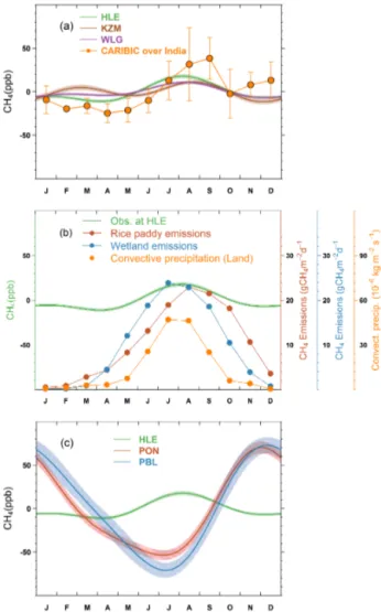
OH. The pronounced HLE feature is consistent with the re-sult from the aircraft flask measurements over India at flight altitudes of 8–12.5 km by the Civil Aircraft for the Reg-ular Investigation of the atmosphere Based on an Instru-ment Container (CARIBIC, http://www.caribic-atmospheric. com/) project (Schuck et al., 2010, 2012; Baker et al., 2012), although a larger seasonal cycle amplitude is found in the CARIBIC composite data due to the rapid vertical mixing over the monsoon region and the strong anticyclone that de-velops in the upper troposphere (Fig. 5a; Schuck et al., 2010). CARIBIC sampled the mid-to-upper tropospheric air masses that were earlier and more strongly enriched in CH4, as a
re-sult of the rapid vertical transport of surface air masses by deep convection and subsequent accumulation and confine-ment of pollutants within the strong, closed circulation of the anticyclone (Li et al., 2005; Randel and Park, 2006). Xiong et al. (2009) also reported enhancements of CH4during the
Figure 3. (a) The mean CO2seasonal cycle at HLE, in compar-ison with the mean seasonal cycles derived from the in situ CO2 measurements over New Delhi at different altitude bands (3–4, 4– 5, and 5–6 km) by the CONTRAIL project (2006–2010). (b) The mean CO2seasonal cycles at HLE, KZM and WLG. (c) The mean CO2seasonal cycles at HLE, PON and PBL. For each station, the mean seasonal cycle is derived from the harmonics of the smoothed fitting curve in Fig. 2. Shaded area indicates the uncertainty of the mean seasonal cycle calculated from 1 SD of 1000 bootstrap repli-cates. For the CONTRAIL data sets, CO2measurements over New Delhi were first averaged by altitude bands. A fitting procedure was then applied to the aggregated CO2measurements to generate the mean season cycle for different altitude bands.
retrievals of CH4 using the Atmospheric Infrared Sounder
(AIRS) on the EOS/Aqua platform as well as model sim-ulations. Moreover, the mean CH4 seasonal cycle at HLE
agrees well with the seasonal variations of CH4 emissions
from wetlands and rice paddies and convective precipita-tion over the Indian subcontinent (Fig. 5b), suggesting that the summer maximum at HLE is likely related to the en-hanced biogenic CH4emissions from wetlands and rice
pad-dies and deep convection that mixes surface emissions into the mid-to-upper troposphere. During the SW monsoon pe-riod (June–September), convection over the Indian subcon-tinent and the Bay of Bengal rapidly mixes surface-polluted air with the upper troposphere, therefore concentrations of trace gases would be enhanced at higher altitudes rather than at the surface (Schuck et al., 2010; Lawrence and Lelieveld, 2010). Further analyses of carbon isotopic measurements and/or chemical transport model are needed to disentangle and quantify the contributions of meteorology and biogenic emissions to the CH4summer maximum at HLE. As stated
above, KZM and WLG also record CH4 increases during
summertime, but with smaller magnitudes (Fig. 5a), possibly because they are not directly influenced by deep convection from the Indian monsoon system.
In contrast to HLE, the CH4mean seasonal cycles at PON
and PBL have distinct phases and much larger amplitudes, with minimum CH4values during July (Fig. 5c). These not
only reflect higher rates of removal by OH, but also the in-fluence of southern hemispheric air transported at low al-titudes from the southwest as well as the dilution effect from the increased local planetary boundary layer height. In boreal winter, the maxima at PON and PBL are associ-ated with CH4-enriched air masses transported from eastern
and northeastern India, and Southeast Asia, mostly polluted by agricultural-related sources (e.g., livestock, rice paddies, agricultural waste burning). As PON and PBL, the flask mea-surements at CRI also showed the seasonal maximum CH4
values during the NE monsoon season, reflecting influences of air masses with elevated CH4from the Indian subcontinent
(Bhattacharya et al., 2009; Tiwari et al., 2013).
3.1.3 N2O
Nitrous oxide (N2O) is a potent greenhouse gas that has the
third largest contribution to anthropogenic radiative forcing after CO2 and CH4 (IPCC, 2013). It has also become the
dominant ozone-depleting substance (ODS) emitted in the 21st century with the decline of chlorofluorocarbons (CFCs) under the Montreal Protocol (Ravishankara et al., 2009). Since the pre-industrial era, atmospheric N2O has increased
rapidly from ∼ 270 to ∼ 325 ppb in 2011 (IPCC, 2013), largely as the result of human activities. Of the several known N2O sources, agricultural activities (mainly through
nitro-gen fertilizer use) are responsible for ∼ 58 % of the global anthropogenic N2O emissions, with a higher share in a
pre-Figure 4. Time series of CH4flask measurements at (a) HLE and PON, (b) HLE and PBL, (c) HLE and KZM, and (d) HLE and WLG. The open circles denote flask data used to fit the smoothed curves, while the crosses denote discarded flask data lying outside 3 times the residual standard deviations from the smoothed curve fits. For each station, the smoothed curve is fitted using Thoning’s method (Thoning et al., 1989) after removing outliers.
dominantly agrarian country like India (∼ 75 %; Garg et al., 2012).
The time series of N2O flask measurements over the
period of 2007–2011 and their smoothed curves are pre-sented in Fig. 6. At HLE, the annual mean N2O
con-centration rose from 322.2 ± 0.1 to 325.2 ± 0.1 ppb during 2007–2011 (Table 1), with a mean annual growth rate of 0.8 ± 0.0 ppb yr−1(r2=0.97, p = 0.001), smaller than that at MLO (1.0 ± 0.0 ppb yr−1, Table 1). At PON and PBL, the annual mean N2O mole fractions are higher than at
HLE by 3.1 ± 0.3 and 3.8 ± 1.7 ppb (Fig. 6, Table 1), re-spectively. The N2O gradients between PON, PBL and HLE
are larger than typical N2O gradients observed between
sta-tions scattered in Europe or in North America. For exam-ple, Haszpra et al. (2008) presented N2O flask
measure-ments at a continental station – Hegyhátsál, Hungary (HUN – 46.95◦N, 16.65◦W, 248 m a.s.l.), from 1997 to 2007. The annual mean N2O mole fraction at HUN was higher than
at Mace Head (MHD) by only 1.3 ppb. We also analyzed N2O time series of flask measurements during 2007–2011
at several European coastal stations – BGU in Spain, FIK in Greece, and LPO in France (Table S6), and the N2O
gradients between these stations and MHD were 1.1 ± 0.2, 0.4 ± 0.1, and 2.1 ± 0.6 ppb, respectively (Fig. S10, Ta-ble S7). In the United States, N2O flask measurements from
the NOAA/ESRL stations at Park Falls, Wisconsin (LEF – 45.95◦N, 90.27◦W, 472 m a.s.l.), Harvard Forest,
Mas-sachusetts (HFM – 42.54◦N, 72.17◦W, 340 m a.s.l.), and a continental, high-altitude station at Niwot Ridge, Colorado (NWR – 40.05◦N, 105.58◦W, 3523 m a.s.l.), also show that the annual mean N2O concentrations at HFM and LEF were
higher than that at NWR by only 0.5 ± 0.1 and 0.3 ± 0.1 ppb, respectively (Fig. S10, Table S7). Additionally, the N2O
con-centrations measured at PON and PBL have a notably higher variability (around the smoothed fitting curve) than that at European and US stations (see relative SDs (RSDs) in Ta-bles 1 and S7). The larger N2O gradient between PON,
PBL and HLE, as well as higher variability at PON and PBL, demonstrate the presence of substantial N2O sources in
South Asia and over the Indian Ocean during the observation period. The in situ measurements at Darjeeling also exhib-ited N2O enhancements to be above the background level,
suggesting significant N2O sources in this region (Ganesan
et al., 2013). These sources may be related to emissions from natural and cultivated soils probably enhanced by extensive use of nitrogen fertilizers, as well as emissions from regions of coastal upwelling in the Arabian Sea (Bange et al., 2001; Garg et al., 2012; Saikawa et al., 2014).
Compared to CO2 and CH4, the seasonal cycle of N2O
is very small due to the long lifetime of ∼ 120 years (Min-schwaner et al., 1993; Volk et al., 1997), and has a larger un-certainty probably because synoptic events are more likely to mask the seasonal signal. At HLE, PON and PBL, the peak-to-peak amplitudes of the N2O seasonal cycle are 0.6 ± 0.1,
Figure 5. (a) The mean CH4 seasonal cycles observed at HLE, KZM and WLG. The mean CH4seasonal cycle derived from air-craft flask measurements by the CARIBIC project is also presented. The CARIBIC flask measurements in the upper troposphere (200– 300 hPa) during 2005–2012 are averaged over the Indian subcon-tinent (10–35◦N, 60–100◦E) by month to generate the mean sea-sonal cycle. The error bars indicate 1 standard deviation of CH4 flask measurements within the month. (b) The seasonal variations of CH4emissions from rice paddies and wetlands over the Indian subcontinent. The CH4emissions from rice paddies are extracted from a global emission map for the year 2010 (EDGAR v4.2, 2011), imposed by the seasonal variation on the basis of Matthews et al. (1991). The CH4 emissions from wetlands are extracted from outputs of a global vegetation model (BIOME4-TG, Kaplan et al., 2006). The seasonal variation of deep convection over the Indian subcontinent is also presented, indicated by convective precipitation obtained from an LMDZ simulation nudged with ECMWF reanal-ysis (Hauglustaine et al., 2004). The CH4emissions and convective precipitation are averaged over the domain 10–35◦N, 70–90◦E to give a regional mean estimate. (c) The mean CH4seasonal cycles observed at HLE, PON and PBL. For each station, the mean sea-sonal cycle is derived from the harmonics of the smoothed fitting curve in Fig. 4. Shaded area indicates the uncertainty of the mean seasonal cycle calculated from 1 SD of 1000 bootstrap replicates.
1.2 ± 0.5, and 2.2 ± 0.6 ppb, respectively (Table 1). HLE displays a N2O maximum in mid-August (Student’s t test,
t =1.78, p = 0.06), and a secondary maximum is in Jan-uary/February but not significant (Student’s t test, t = −0.84,
p =0.79) (Table 1, Fig. 7, Table S8 for detailed t test statis-tics). The N2O seasonal cycle at HLE is out of phase with
that at other northern background stations such as MHD (Fig. S11, Table S7), where an N2O summer minimum is
al-ways observed, likely due to the downward transport of N2
O-depleted air from the stratosphere to the troposphere during spring and summer (Liao et al., 2004; Morgan et al., 2004; Jiang et al., 2007b). The timing of the summer N2O
maxi-mum at HLE is consistent with that of CH4(Table 1; Figs. 5
and 7), giving evidence that the N2O seasonal cycle is
proba-bly influenced by the convective mixing of surface air, rather than by the influx of stratospheric air into the troposphere. Given that the populous Indo-Gangetic Plain has high N2O
emission rates due to the intensive use of nitrogen fertiliz-ers (Garg et al., 2012; Thompson et al., 2014a), during sum-mer, the surface air enriched in N2O is vertically transported
by deep convection and enhances N2O mole fractions in the
mid-to-upper troposphere. Like CH4, the N2O enhancement
during the summer monsoon period (June–September) was also observed by the aircraft flask measurements at flight alti-tudes 8–12.5 km from the CARIBIC project in 2008 (Schuck et al., 2010).
At PON, N2O also decreases during February–April and
reaches a minimum at the end of May. However, the decrease of N2O does not persist during June–September, which is in
contrast with CH4(Table 1, Fig. 7a). One reason may be that
the air masses arriving at the site during the southwest mon-soon period is relatively enriched in N2O compared to CH4,
reflecting differences in their relative emissions along the air mass route. The increase of N2O at PON during June–August
and the maximum during September–October are likely re-lated to N2O emissions from coastal upwelling along the
southern Indian continental shelf, which peak during the SW monsoon season (Patra et al., 1999; Bange et al., 2001). Ac-cording to Bange et al. (2001), the annual N2O emissions for
the Arabian Sea are 0.33–0.70 Tg yr−1, of which N2O
emis-sions during the SW monsoon account for about 64–70 %. This coastal upwelling N2O flux is significantly larger than
the annual anthropogenic N2O emissions in southern India
south of 15◦N, which is estimated to be on average 0.07– 0.08 Tg yr−1 during 2000–2010 (EDGAR v4.2, 2011). At PBL, the maximum and minimum N2O occur in November
and February/March, respectively (Table 1, Fig. 7b). The late N2O peak at PBL in November might be associated with the
N2O-enriched air masses transported from South and
South-east Asia, which could be attributed to natural and agricul-tural N2O emissions from this region (Saikawa et al., 2014).
It should be noted that the mean seasonal cycles of N2O at
PON and PBL are subject to high uncertainties because of the short observation periods and data gaps (shaded area in Fig. 7). The N2O maximum and/or minimum obtained from
Figure 6. Time series of N2O flask measurements at (a) HLE and PON and (b) HLE and PBL. The open circles denote flask data used to fit the smoothed curves, while crosses denote discarded flask data lying outside 3 times the residual standard deviations from the smoothed curve fits. For each station, the smoothed curve is fitted using Thoning’s method (Thoning et al., 1989) after removing outliers.
Figure 7. The mean N2O seasonal cycles observed at (a) HLE and PON and (b) HLE and PBL. For each station, the mean seasonal cycle is derived from the harmonics of the smoothed fitting curve in Fig. 6. Shaded area indicates the uncertainty of the mean seasonal cycle calculated from 1 SD of 1000 bootstrap replicates.
the mean seasonal cycle are marginally significant for PON and PBL (Table S8 for detailed t test statistics). Therefore, caution should be exercised in interpreting mean seasonal cycles at these stations. Sustained, long-term measurements are needed in order to generate more reliable estimates of the seasonal cycles for the two stations.
3.1.4 SF6
Sulfur hexafluoride (SF6)is an extremely stable greenhouse
gas, with an atmospheric lifetime as long as 800–3200 years and a global warming potential (GWP) of ∼ 23 900 over a 100-year time horizon (Ravishankara et al., 1993; Morris et al., 1995; IPCC, 2013). The main sources of atmospheric SF6 emissions are electricity distribution systems,
magne-sium production, and semi-conductor manufacturing (Olivier et al., 2005), while its natural sources are negligible (Busen-berg and Plummer, 2000). As its sources are almost purely anthropogenic (Maiss et al., 1996), SF6is widely considered
as a good tracer for population density, energy consumption and anthropogenic GHG emissions (Haszpra et al., 2008).
Figure 8 presents the time series of SF6 flask
mea-surements and corresponding fitting curves at HLE, PON, and PBL. At HLE, the annual mean SF6 mole
frac-tions increased from 6.26 ± 0.03 to 7.38 ± 0.01 ppt be-tween 2007 and 2011, which is in good agreement with the SF6 trend observed at MLO during the same period
(HLE: 0.29 ± 0.05 ppt yr−1, r2=0.99, p < 0.001; MLO: 0.29 ± 0.03 ppt yr−1, r2=0.99, p < 0.001; Figs. 8 and S12a, Tables 1, S9). The annual mean SF6 gradient between
PON and HLE is −0.060 ± 0.030 ppt, whereas the gra-dient between PBL and HLE is statistically insignificant (−0.002 ± 0.097 ppt). The slight negative gradient between PON and HLE is a reversed signal compared with the SF6
observations at stations influenced by continental emissions in Europe and United States. For example, the SF6 mole
fractions at HUN over the years of 1997–2007 are higher than those at MHD by on average 0.19 ppt (Haszpra et al., 2008). We also analyzed the SF6 gradients (relative to
MHD) for two European stations – BGU (41.97◦N, 3.30◦E, 30 m a.s.l.) and LPO (48.80◦N, 3.57◦W, 30 m a.s.l.), which are 0.10 ± 0.03 and 0.05 ± 0.02 ppt averaged over the pe-riod of 2007–2011, respectively. At HFM, the SF6 mole
Figure 8. Time series of SF6flask measurements at (a) HLE and PON and (b) HLE and PBL. The open circles denote flask data used to fit the smoothed curves. For each station, the smoothed curve is fitted using Thoning’s method (Thoning et al., 1989) after removing outliers.
fractions are higher than those of the NWR on average by 0.15 ± 0.06 ppt during 2007–2011 (Table S9). Given the long atmospheric lifetime of SF6, the positive gradients between
continental European and US stations and background refer-ence stations suggest significant sources in Europe and the US. The slight negative gradient between PON and HLE implies weak SF6 emissions over the Indian subcontinent,
which is also indicated by recent high-frequency in situ SF6
measurements at Darjeeling (Ganesan et al., 2013). It is also worthwhile to note that high SF6values occur repeatedly at
HLE and PBL in winter, which is likely related to episodic SF6pollution events from the Middle East, South/Southeast
Asia and China (Figs. 8b and S7d).
The annual mean SF6 seasonal cycles for HLE, PON,
and PBL are presented in Fig. 9. The peak-to-peak ampli-tudes at the three stations are 0.15 ± 0.03, 0.24 ± 0.02, and 0.48 ± 0.07 ppt, respectively (Table 1). At HLE, the SF6
sea-sonal cycle is bimodal as for N2O, with an absolute
max-imum occurring in November (Student’s t test, t = 2.425,
p =0.014) and a secondary maximum in May (Student’s
t test, t = 2.443, p = 0.016) (Table S10 for detailed t test statistics). Given that SF6increases monotonously and that
its sources are purely anthropogenic and not subject to sea-sonally variations (Maiss et al., 1996), the seasonal cycle of SF6 should be driven by changes in atmospheric
circu-lations, e.g., the SW monsoon convection and stratosphere– troposphere exchange (Levin et al., 2002). We note that, at HLE, no enhancement of SF6during the SW monsoon
sea-son is recorded, unlike what is observed for CH4and N2O
(Figs. 5 and 7). Although the CARIBIC aircraft flask mea-surements over the Indian region demonstrated SF6
enhance-ments in the upper troposphere at ∼ 30◦N (approximately where HLE is located) in August, 2008, they are not related to the deep convection and surface sources that contribute to the summer maxima in CH4and N2O. Back trajectories from
the CARIBIC flights showed that the summer enhancements in SF6were related to air samples collected north of 20◦N
along the flight routes, where air masses were more
influ-enced by the westerly subtropical jet (and a smaller anticy-clone embedded in it over the Arabian Peninsula) rather than the deep convection in the monsoon region (Krishnamurti et al., 2008; Schuck et al., 2010; Fig. S9). Since HLE is not influenced by the westerly subtropical jet in the upper tropo-sphere (also clearly seen by the colors of back trajectories in Fig. S9), the summer enhancements of SF6observed by the
CARIBIC flights are not detected by the flask measurements at HLE. The absence of SF6enhancement in summer at HLE
confirms weak SF6emissions in India. At PBL, the SF6
sea-sonal cycle is related to the monsoon circulation and convec-tion (Figs. 9b and S7d). The maximum during November– December (Student’s t test, t = 5.138, p < 0.001; Table S10) is likely due to frequent episodic SF6-polluted air masses
transported from Southeast Asia and China (Fig. S7d).
3.1.5 CO
Carbon monoxide (CO) plays important roles in atmospheric chemistry, as the dominant sink for the hydroxyl radical (OH, the main tropospheric oxidant) and a precursor of tropo-spheric ozone under high NOx (NO+NO2)concentrations
(Logan et al., 1981; Novelli et al., 1998; Seinfeld and Pan-dis, 2006). Although CO does not act as a greenhouse gas, it modulates the atmospheric concentrations of CH4 (the
second most abundant anthropogenic greenhouse gas after CO2)through competition for the OH radicals. At the global
scale, it contributes to an indirect positive radiative forc-ing of 0.23 ± 0.07 W m−2(IPCC, 2013). Additionally, CO is
an excellent tracer for combustion processes, with emission sources mainly contributed by incomplete combustion of fos-sil fuel and biofuels, and by biomass burning (Granier et al., 2011). In India, biofuel and agricultural waste burning ac-count for 70–80 % of the total anthropogenic CO emissions (EDGAR v4.2, 2011; Streets et al., 2003b; Yevich and Lo-gan, 2003).
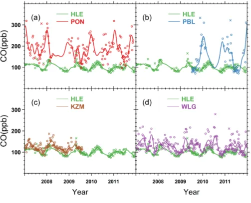
The time series of CO flask measurements and correspond-ing smoothed curves are shown in Fig. 10. Over the period
Figure 9. The mean SF6seasonal cycles observed at (a) HLE and PON and (b) HLE and PBL. For each station, the mean seasonal cycle is derived from the harmonics of the smoothed fitting curve in Fig. 8. Shaded area indicates the uncertainty of the mean seasonal cycle calculated from 1 SD of 1000 bootstrap replicates.
Figure 10. Time series of CO flask measurements at (a) HLE and PON, (b) HLE and PBL, (c) HLE and KZM, and (d) HLE and WLG. The open circles denote flask data used to fit the smoothed curves, while the crosses denote discarded flask data lying outside 3 times the residual standard deviations from the smoothed curve fits. For each station, the smoothed curve is fitted using Thoning’s method (Thoning et al., 1989) after removing outliers.
of 2007–2011, HLE recorded a slight decrease in CO mole fractions from 104.7 ± 1.4 to 99.4 ± 2.2 ppb, with an annual rate of −2.2 ± 0.0 ppb yr−1 (r2=0.65, p = 0.06). The CO mole fractions at HLE are lower than those at KZM and WLG (Novelli and Masarie, 2014), by on average 18.8 ± 2.5 and 30.2 ± 7.4 ppb, respectively (Table 1, Fig. 10c and d). The positive gradient between KZM, WLG and HLE not only reflects decreasing CO with altitude and the N–S global gradient, but also suggests differences in regional emission
sources. For example, compared to HLE, the CO signals at WLG are more influenced by transport of polluted air, es-pecially during summer when about 30 % air masses pass over industrialized and urbanized areas southeast of the sta-tion (Zhang et al., 2011). Addista-tionally, the positive CO gradi-ent between KZM, WLG and HLE may be further increased by air masses of northern Siberia origin in summer (Fig. S5), with higher CO emissions from biomass burning and sec-ondary CO from the oxidation of CH4and non-CH4
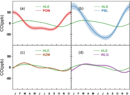
hydro-Figure 11. The mean CO seasonal cycles observed at (a) HLE and PON, (b) HLE and PBL, (c) HLE and KZM, and (d) HLE and WLG. For each station, the mean seasonal cycle is derived from the harmonics of the smoothed fitting curve in Fig. 10. Shaded area indicates the uncertainty of the mean seasonal cycle calculated from 1 SD of 1000 bootstrap replicates.
carbons (Konovalov et al., 2014). At PON and PBL, the an-nual mean CO mole fractions are higher than that at HLE by on average 82.4 ± 10.7 and 52.5 ± 8.5 ppb, respectively (Table 1, Fig. 10a and b). The PON and PBL stations are influenced by CO regional emissions, mainly due to bio-fuel and agricultural burning over South and Southeast Asia (Lelieveld et al., 2001; Streets et al., 2003a, b; Yevich and Logan, 2003). We also note that, for all five stations, the CO time series show larger variability with respect to their cor-responding smoothed curves than other species do (see the residual SD (RSD) in Table 1, Fig. 10), as a result of the un-evenly distributed CO sources and short atmospheric lifetime (Novelli et al., 1992).
As shown in Fig. 11, the CO seasonal cycle at HLE reaches a maximum in mid-March and a minimum by the end of Oc-tober, with a peak-to-peak amplitude of 28.4 ± 2.3 ppb (Ta-ble 1, Fig. 11). The phase of the mean CO seasonal cycle at HLE generally agrees with the ones observed at KZM and WLG, with a lag of up to 1 month in the timing of seasonal minimum at the two stations (Table 1, Fig. 11c and d). In con-trast with the three stations representative of large-scale free tropospheric air masses, the stations at the maritime bound-ary layer in the mid-to-high Northern Hemisphere observe the lowest CO values in July or August (Novelli et al., 1992, 1998), when the concentration of OH – the major sink of CO – is highest (Logan et al., 1981). The delay in timing of the seasonal CO minimum at the three free troposphere stations in Central and South Asia compared to those boundary layer stations is probably due to the mixing time of regional
sur-face CO emissions and the relatively short lifetime of CO (1–2 months on average). During summer, KZM and WLG sample air masses from Siberia impacted by CO fire emis-sions (Duncan et al., 2003; Kasischke et al., 2005), and CO-polluted air from urbanized and industrialized areas (Zhang et al., 2011), while HLE is influenced by convective mix-ing of CO emissions from India, either from anthropogenic sources or oxidation of volatile organic compounds. It is in-teresting to note that the CO seasonal cycle at HLE does not show an enhancement during JAS as CH4and N2O do
(Figs. 5 and 7), possibly as a result of OH oxidation that reduces CO and acts oppositely to vertical transport, and/or differences in seasonal emission patterns between CO and the other two species (Baker et al., 2012). However, the CO enhancement during summer was observed in the upper tro-posphere over South Asia from the CARIBIC aircraft mea-surements at flight altitudes 8–12.5 km and Microwave Limb Sounder observations at 100–200 hPa (Li et al., 2005; Jiang et al., 2007a; Schuck et al., 2010). The differences in the CO seasonal cycles at different altitudes suggest faster transport (and younger air masses) at 10 km than at 5 km due to con-vection, controlling the vertical profile of CO, which makes it difficult to directly compare aircraft measurements in the upper troposphere and column remote sensing observations with surface data.
At PON and PBL, the mean CO seasonal cycles show maxima in the boreal winter and minima in the boreal summer, with peak-to-peak amplitudes of 78.2 ± 11.6 and 144.1 ± 16.0 ppb, respectively (Fig. 11a and b). A strong