HAL Id: hal-00368844
https://hal.archives-ouvertes.fr/hal-00368844
Preprint submitted on 17 Mar 2009HAL is a multi-disciplinary open access
archive for the deposit and dissemination of sci-entific research documents, whether they are pub-lished or not. The documents may come from teaching and research institutions in France or abroad, or from public or private research centers.
L’archive ouverte pluridisciplinaire HAL, est destinée au dépôt et à la diffusion de documents scientifiques de niveau recherche, publiés ou non, émanant des établissements d’enseignement et de recherche français ou étrangers, des laboratoires publics ou privés.
Dynamical Analysis of a new statistically highly
performant deterministic function for chaotic signals
generation
Sebastien Hénaff, Ina Taralova, René Lozi
To cite this version:
Sebastien Hénaff, Ina Taralova, René Lozi. Dynamical Analysis of a new statistically highly performant deterministic function for chaotic signals generation. 2009. �hal-00368844�
Dynamical Analysis of a new statistically highly performant
deterministic function for chaotic signals generation
S´ebastien H´enaff, Ina Taralova
IRCCyN, UMR CNRS 6597, ´Ecole Centrale Nantes, 1 rue de la No¨e, BP 92101, F-44321 Nantes
Cedex 3, France Ren´e Lozi
Laboratoire J.A. Dieudonn´e, UMR CNRS 6621, Universit´e de Nice Sophia-Antipolis, 06108 Nice Cedex 02, France
1
Introduction
In some engineering applications, such as chaotic encryption, chaotic maps have to exhibit required spectral and statistical properties close to those of random signals [1] [2]. In order to evaluate the latter features, statistical tests developed for random number generators (RNG) can also be applied to chaotic maps, in order to gather evidence that the map generates ”good” chaotic signals, i.e. having a considerable degree of randomness. To address this particular problem, different statistical tests for the systematic evaluation of the randomness of cryptographic random number generators can be applied, among which the most popular NIST (National Institute of Standards and Technology) [3] tests. In this paper we present the analysis of a new ultra weakly coupled maps system introduced by Lozi in [4]. This paper is organised as follow : section two presents the considered map. Section three study its statistical properties and section four study its evolution with parameter variation. A conclusion ends this paper.
2
System under study
In [4], a new coupled map system was introduced. The Nth order function F under consideration
can be written as : (x1(n + 1), x2(n + 1), . . . , xN(n + 1)) = F (x1(n), x2(n), . . . , xN(n)) x1(n + 1) x2(n + 1) .. . xN(n + 1) = 1 − (N − 1)ǫ1 ǫ1 . . . ǫ1 ǫ2 1 − (N − 1)ǫ2 . . . ǫ2 .. . ... . .. ... ǫN ǫN . . . 1 − (N − 1)ǫN Λ(x1(n)) Λ(x2(n)) .. . Λ(xN(n)) (1)
where Λ is the triangular function.
As introduced by Lozi in [4], the maps are weakly coupled choosing ǫ1 = 10−14 et ǫi = iǫ1. The
states evolves in the interval : [−1; 1]N. In the definition, the output signal ¯x to be transmitted is
constructed choosing a particular sampling of the states {x1; x2; ...; xn} of the system F :
¯ x(q) = x1(n) if xN(n) ∈ [T1, T2] x2(n) if xN(n) ∈ [T2, T3] .. . xN −1(n) if xN(n) ∈ [TN −1, 1] (2)
with −1 < T1 < T2< ... < TN −1. q denotes the index of the signal ¯x and n is associated to the
original map F . The notation n(q) is used to represent the index of the original map. The index
of the generated pseudo-random signal in such a way that for a second order, ¯x(q) = x1(n(q)).
3
System Analysis
3.1 SignalThe spectrum X of a signal x is defined as :
X(k) = F T (x)(k)
The spectrum of the signal x1 generated is represented in figure 1. It can be quantified by
0 200 400 600 800 1000 0 500 1000 1500 2000 2500 Figure 1: spectrum X1
the autocorrelation of the signal. The correlation of two real signals x and y is calculated by the following expression :
Γxy(τ ) =
X
n
x(n + τ )y(n)
it is related to the spectra X and Y of the signals x and y by the relation :
Γxy = T F−1(XY∗)
The autocorrelation Γx is plotted in figure 2. The autocorrelation of a pseudo-random signal is
close to a Dirac peak. The tests which have been carried out show that the system generates a wide-band signal before, as well as after the sampling of equation (2). The presented curves are those of the signal before the sampling.
0 200 400 600 800 1000 0 0.2 0.4 0.6 0.8 1 Figure 2: autocorrelation of x1 3.2 Lyapunov Exponents
The Lyapunov Exponents (LE) quantify the sensitivity to the initial conditions using the average
of the Jacobians matrix. If f′
is the Jacobian matrix, then, the Lyapunov exponents are :
λi= lim N →∞ 1 N ln |vpi(f ′ (x(N ))f′(x(N −1))...f′(x(1)))|
where f is the investigated function, f′
is the corresponding Jacobian, and x represents the system
state. The signal xN is uniformly distributed in the interval [−1, 1], therefore we select in average
one point out of hundred iterates if T1 = 0.98. The LE of the global system have to be redefined.
To do this, let consider the system H, defined in second order by :
H : (y1(q + 1), y2(q + 1)) = H(y1(q), y2(q))
The states (y1; y2) are defined by : y1(q) = x1(n(q)) et y2(q) = x2(n(q)). In other words, only
the states of F remaining after the sampling (2) are kept. The values used for the simulations are
the following : considering the second order function, T1 = 0.98, with the third order function,
(T1, T2) = (0.98, 0.99) and with the fourth order function , (T1, T2, T3) = (0.98, 0.987, 0.993). The
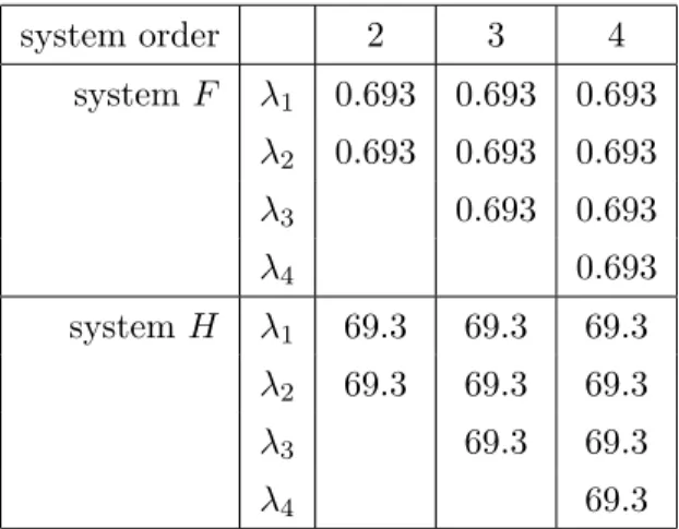
results are the same whatever the initial conditions, since the chaotic attractor fills entirely the phase space. Table 1 compares the Lyapunov Exponent values for different system orders. This value does not vary with the system order, but is increased by a factor of one hundred when the global system (2) is considered, taking into account that approximately one point out of 100 iterates is kept. The LE are defined as the speed of deviation of two trajectories initialised in the same vicinity. Therefore the LE of F oF should be twice bigger compared to the LE of F . Keeping in mind that the iterates of (1) are in average selected one out of hundered, then the LE of H are one hundered times more important as shown in table 1.
3.3 Signal repartition analysis
According to [4], the following quantifiers are used :
1) Ec1 : Norm L1 of the deviation between the signal distribution and the uniform distribution
2) Ec2 : Deviation from the uniform distribution according to the norm L2
The quantifiers are used for the signal repartition analysis in all dimensions. The table 2 com-pares the signal distributions for different system dimensions. In order to have comparable results, a histogram with a constant number of intervals has to be considered whatever the dimension of the phase space. For this kind of histogram, the results are identical whatever the dimension.
The second test compares the signal distributions in the phase space(x ,x ), p ∈ [1; 1000] and
Table 1: Lyapunov exponents value system order 2 3 4 system F λ1 0.693 0.693 0.693 λ2 0.693 0.693 0.693 λ3 0.693 0.693 λ4 0.693 system H λ1 69.3 69.3 69.3 λ2 69.3 69.3 69.3 λ3 69.3 69.3 λ4 69.3
Table 2: system distribution vs distribution dimension
dimension Ec1 Ec2 2 1, 7.10−5 1, 38.10−3 3 1, 7.10−5 1, 38.10−3 4 1, 8.10−5 1, 40.10−3 6 1, 7.10−5 1, 38.10−3 7 1, 8.10−5 1, 42.10−3
standard deviation is between 10.9 and 11.8, Ec1 is between 1.710−5 and 1.810−5. Ec2 is between
1.3310−3
and 1.4410−3
. Finally, we don’t notice a significant deviation, the distributions remaining homogeneous.
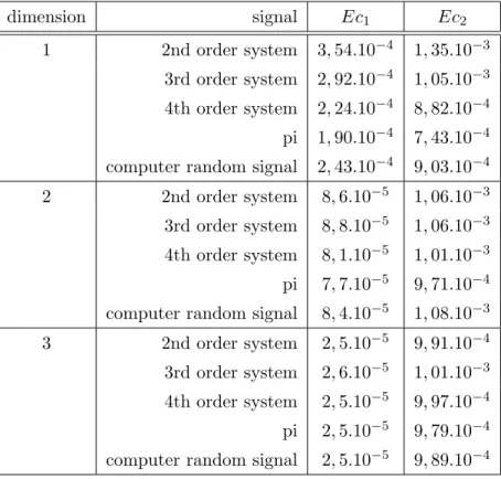
The third test in table 3 consists in comparing the results for different systems. The first signal is the signal under investigation, the second is the signal composed of the numbers of pi, and the third is a random signal generated by matlab. The calculation of the histogram is adapted to the specificity of the signal pi : it is calculated over 10 intervals by dimension, which explains the differences between the obtained values and the previous ones, but also the differences between two dimensions.
Table 3: distribution comparaison in fonction of systems
dimension signal Ec1 Ec2 1 2nd order system 3, 54.10−4 1, 35.10−3 3rd order system 2, 92.10−4 1, 05.10−3 4th order system 2, 24.10−4 8, 82.10−4 pi 1, 90.10−4 7, 43.10−4
computer random signal 2, 43.10−4
9, 03.10−4 2 2nd order system 8, 6.10−5 1, 06.10−3 3rd order system 8, 8.10−5 1, 06.10−3 4th order system 8, 1.10−5 1, 01.10−3 pi 7, 7.10−5 9, 71.10−4
computer random signal 8, 4.10−5
1, 08.10−3 3 2nd order system 2, 5.10−5 9, 91.10−4 3rd order system 2, 6.10−5 1, 01.10−3 4th order system 2, 5.10−5 9, 97.10−4 pi 2, 5.10−5 9, 79.10−4
computer random signal 2, 5.10−5
9, 89.10−4
3.4 Hurst exponents
The Hurst exponents quantify the repetitivity (short) of a long time evolving sequence. They are calculated by the expression :
R/S(n) =
n
X
k=1
(s(k) − s)
The Hurst exponent is then defined as being the slope of the curve ln(R/S)/ln(n). An exponent equal to 0.5 indicates that the signal is random. If the exponent is H > 0.5, the signal is said to be persistent, and its points have a tendency to follow the previous one. If H < 0.5, the signal is anti-persistent, this is the opposite case. The Hurst exponents have been calculated for the three different systems as shown in table 4. Finally, the studied system presents the same caracteristics
Table 4: Hurst exponents
signal 30 000 points 100 000 points
2nd order system 0.509 0.530
3rd order system 0.514 0.522
4th order system 0.511 0.528
pi 0.549 0.522
computer random signal 0.522 0.510
3.5 Statistical Analysis
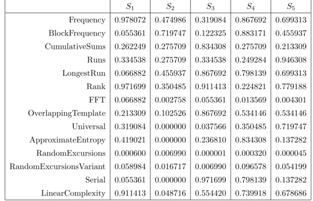
The National Institute of Standards and Technology (NIST) has developed a statistical test suite for the systematic evaluation of the randomness of cryptographic random number generators (RNG) [3]. These tests are statistical tests which allow to investigate the degree of randomness for binary sequences produced by random number generators (RNG). The presented tests are applied over 100 series of data of the system (2) composed of 1 000 000 points. The sequence validates the tests if each small series validates a list of elementary tests for exemple the spectrum distribution, the long term redundancy. The data appearing in table 5 represent the probability that the analyzed data are random so ideally, all probabilities are equal to one. Certain tests propose several different probabilities, and only the worst (i.e. the weakest) ones are reported.
Table 5: NIST tests
S1 S2 S3 S4 S5 Frequency 0.978072 0.474986 0.319084 0.867692 0.699313 BlockFrequency 0.055361 0.719747 0.122325 0.883171 0.455937 CumulativeSums 0.262249 0.275709 0.834308 0.275709 0.213309 Runs 0.334538 0.275709 0.334538 0.249284 0.946308 LongestRun 0.066882 0.455937 0.867692 0.798139 0.699313 Rank 0.971699 0.350485 0.911413 0.224821 0.779188 FFT 0.066882 0.002758 0.055361 0.013569 0.004301 OverlappingTemplate 0.213309 0.102526 0.867692 0.534146 0.534146 Universal 0.319084 0.000000 0.037566 0.350485 0.719747 ApproximateEntropy 0.419021 0.000000 0.236810 0.834308 0.137282 RandomExcursions 0.000600 0.006990 0.000001 0.000320 0.000045 RandomExcursionsVariant 0.058984 0.016717 0.006990 0.096578 0.054199 Serial 0.055361 0.000000 0.971699 0.798139 0.137282 LinearComplexity 0.911413 0.048716 0.554420 0.739918 0.678686
In the notation of the table, the system S1 represents the forth order system, with parameters
ǫ1 = 10−9 and a sampling T1 = 0.99. The system S2 represents the forth order system, with
parameters ǫ1 = 10−9 and the sampling T1 = 0.9. The third system S3 is a fourth order one with
parameters ǫ1 = 10−5 and a sampling T1 = 0.99. The other parameters of the three previous
systems are defined by ǫi = iǫ1 and the parameters T2 et T3 are defined in order to distribute them
equitably in the space [T1; 1]. Finally S4 et S5 are respectively generated by the function random
of the computer and by the Frey system [5].
By comparing S1 and S2, the results show that the data series generated by the system (1) are
improved when the sampling is more selective, which goes in the same sense that the Lyapunov exponents analysis. On the other hand, the system exhibits properties comparable to the random generator of the computer and the system of Frey.
4
Parameter analysis
All the previous statistical analyses have been carried out for a particular parameter values. How-ever, in order to be used in chaotic encryption, the system has to exhibit desirable properties for a large set of parameter values (which form the encryption key). This section aims at determin-ing which is the set of acceptable parameter values. From the definition, the system (1) can be
used only in the parameter space ǫk ∈ [0;N1] where N is the order of the system in such a way
that the system states remain in the space [−1; 1] but the statistical criteria (signal distribution, spectrum) as well as the ones from the dynamical systems theory (sensitivity to the initial condi-tions, parameter sensitivity) have to bring additional conditions to define the acceptable parameter regions.
4.1 Signal distribution
The uniform distribution of a pseudo-random signal is an elementary feature. The analysis of the signal distribution generated by (1) for small parameter values have already been studied in [4] but our purpose here is to study the same system for a large set of parameter values. In this case, the property of uniform distribution has to be satisfied on the whole domain where the function is defined. However, by varying the parameter combinations, the features have been deteriorated.
The evolution of the signal values generated for increasing ǫ1 values is represented in figure 3. When
the parameter ǫ1 becomes higher than 10−3, the generated signal does not fulfill the whole interval
[−1; 1]. That’s why tests of validity of distribution uniformity are carried out in order to determine an exploitable parameter space.
The approach consists in applying the same tests as the ones presented in [4] but for a larger set of parameter values. Following this criterion, the system parameters have to remain smaller
than 10−3
so that the distribution of the points was uniform.
4.2 Lyapunov exponents evolution and bifurcations
The analysis of the Lyapunov exponents allows to identify, among others, the parameter regions exhibiting bifurcations. In order to identify them, the Lyapunov exponents have been calculated for a set of parameters. A sudden change of their values would indicate a bifurcation. The simulations show that the Lyapunov exponents vary continuously, which excludes bifurcations in the selected parameter space, as shown in figure 4. The set of simulations is carried out in the parameter space
ǫ1 ∈ [0; 0.1] and ǫ2 = 2ǫ3 = 4ǫ4 = 4.10−5 for the third order system. In this figure, the three
10−5 10−4 10−3 10−2 10−1 −1 −0.5 0 0.5 1
Figure 3: Signal evolution x1 for ǫ1 ∈ [10−5; 0.25], (ǫ2, ǫ3, ǫ4) = (10−3, 10−4, 10−5)
0 0.01 0.02 0.03 0.04 0.05 0.06 0.07 0.08 0.09 0.1 0.65 0.7 0.75 0.8 0.85 0.9 0.95 λ1 λ2 λ3 λ4
Figure 4: Lyapunov exponents evolution ǫ1 ∈ [0; 0.1],ǫ2= 2ǫ3= 4ǫ4 = 4.10−5
5
Conclusion
This paper presented the dynamical and statistical analysis of a weakly coupled maps system introduced by Lozi. The model is a deterministic one, but exhibits spectral properties (spectrum, correlation and autocorrelation) close to those of random signals, and successfully passed all the statistical tests for closeness to random signals (NIST). In addition, if a particular sampling is applied, the Lyapunov exponent is shown to increase. The analyses of the spectral properties, the statistical (NIST) tests, the signal repartition and the Hurst exponents show very satisfactory results. In addition, it can be concluded that the data series generated by the system (1) are improved when the sampling is more selective, which goes in the same sense that the Lyapunov exponents analysis. Finally, is can be concluded that the proposed system exhibits properties comparable to those of the random number generators.
References
[1] G. Alvarez and S. Li, Some Basic Cryptographic Requirements for Chaos-Based Cryptosystems. International Journal of Bifurcation and Chaos (IJBC), Vol. 16 (2006), Pages 2129-2151. [2] H. Noura, S. H?naff, I. Taralova and S. El Assad Efficient cascaded 1-D and 2-D chaotic
gen-erators. Second IFAC Conference on Analysis and Control of Chaotic Systems, (2009)
[3] A. Rukhin, J. Soto, J. Nechvatal, M. Smid, E. Barker, S. Leigh, M. Levenson, M. Vangel, D. Banks, A. Heckert, J. Dray, S. Vo, A statistical test suite for pseudorandom numbers for cryptographic applications, NIST Special Publication Vol. 366 (2001)
[4] R. Lozi, New enhanced chaotic number generators. Indian journal of industrial and applied mathematics, Vol. 1 No. 1 (2008), Pages 1-23.
[5] D.R.Frey, Chaotic digital encoding: an approach to secure communication. IEEE Trans.Circuits Syst. II, Volume 40, Issue 10 (1993), Pages 660-666.
![Figure 3: Signal evolution x 1 for ǫ 1 ∈ [10 − 5 ; 0.25], (ǫ 2 , ǫ 3 , ǫ 4 ) = (10 − 3 , 10 − 4 , 10 − 5 )](https://thumb-eu.123doks.com/thumbv2/123doknet/13050294.383012/9.892.207.698.242.442/figure-signal-evolution-x-ǫ-ǫ-ǫ-ǫ.webp)
