Automated feature extraction in oceanographic visualization

Automated Feature Extraction in Oceanographic

Visualization

by

Da Guo

Submitted to the Department of Ocean Engineering

in partial fulfillment of the requirements for the degrees of

Master of Science in Ocean Engineering

and

Master of Science in Electrical Engineering and Computer Science

at the

MASSACHUSETTS INSTITUTE OF TECHNOLOGY

February 2004

@

Massachusetts Institute of Technology 2004. All rights reserved.

A u th o r ...

... ...

Department of Ocean Engineering

December 22, 2003

Certified by ...

...

Nicholas M. Patrikalakis

Kawasaki Professor of Engineering

Thesis Supervisor

C ertified by ... ..

...

Seth Teller

X-Consortium Associate Profepsofi of o puter 'ience & Engineering

esis Reader

Certified by...

Michael S. Triantafyllou

Chairman, Department Coumittee oi-Gyaluate S)udents

C ertified by ...

Chairman, Department Committee

Arthur C. Smith

on Graduate Students

SEP

0 1

2005

BARKER

-Automated Feature Extraction in Oceanographic

Visualization

by

Da Guo

Submitted to the Department of Ocean Engineering on December 22, 2003, in partial fulfillment of the

requirements for the degrees of Master of Science in Ocean Engineering

and

Master of Science in Electrical Engineering and Computer Science

Abstract

The ocean is characterized by a multitude of powerful, sporadic biophysical dynamical events; scientific research has reached the stage that their interpretation and predic-tion is now becoming possible. Ocean predicpredic-tion, analogous to atmospheric weather prediction but combining biological, chemical and physical features is able to help us understand the complex coupled physics, biology and acoustics of the ocean.

Applications of the prediction of the ocean environment include exploitation and management of marine resources, pollution control such as planning of maritime and naval operations. Given the vastness of ocean, it is essential for effective ocean pre-diction to employ adaptive sampling to best utilize the available sensor resources in order to minimize the forecast error. It is important to concentrate measurements to the regions where one can witness features of physical or biological significance in progress. Thus automated feature extraction in oceanographic visualization can facil-itate adaptive sampling by presenting the physically relevant features directly to the operation planners. Moreover it could be used to help automate adaptive sampling.

Vortices (eddies and gyres) and upwelling, two typical and important features of the ocean, are studied. A variety of feature extraction methods are presented, and those more pertinent to this study are implemented, including derived field generation and attribute set extraction. Detection results are evaluated in terms of accuracy, computational efficiency, clarity and usability.

Vortices, a very important flow feature is the primary focus of this study. Several point-based and set-based vortex detection methods are reviewed. A set-based vortex core detection method based on geometric properties of vortices is applied to both classical vortex models and real ocean models. The direction spanning property, which is a geometric property, guides the detection of all the vortex core candidates, and the conjugate pair eigenvalue method is responsible for filtering out the false positives from the candidate set. Results show the new method to be analytically accurate and practically feasible, and superior to traditional point-based vortex detection methods.

Detection methods of streamlines are also discussed. Using the novel cross method or the winding angle method, closed streamlines around vortex cores can be detected. Therefore, the whole vortex area, i.e., the combination of vortex core and surrounding streamlines, is detected. Accuracy and feasibility are achieved through automated vortex detection requiring no human inspection. The detection of another ocean

feature, upwelling, is also discussed.

Thesis Supervisor: Nicholas M. Patrikalakis Title: Kawasaki Professor of Engineering Thesis Reader: Seth Teller

Acknowledgments

I would like to express my heartfelt thanks to the following people for their support

in this research project:

Professor Nicholas M. Patrikalakis, for his expert advice on my research, instruc-tive guidance on my academic study and words of encouragement. His influence goes beyond this study - he helped me to shape both my academic and life perspectives. Truly the best mentor one can ever imagine.

Professor Seth Teller, for taking time to read my thesis and providing valuable feedback.

Dr. Constantinos Evangelinos, for his acute academic insights and continuous guidance in my research work. His devotion to research work is contagious to me and my labmates.

I am also grateful to Dr. P. Haley and Dr. P. F. J. Lermusiaux, who provided me HOPS data models and were generous and patient to answer my questions.

Special thanks go to Mr. Fred Baker, for providing a stable hardware environment for my thesis work, and to Dr. Qiang Zhu, for his valuables perspectives regarding vortex detection.

I also want to thank my fiancee, Kun, for her love, understanding and support

during my study at MIT; and to my friends, including Dr. Kwang Hee Ko and Dr. Yingbin Bao, many thanks for their valuable ideas and suggestions.

Lastly, my parents, who have been offering me unyielding support as always - to them this work is dedicated.

This work was funded in part from NSF/ITR under grant No. EIA-0121263 and NOAA/Sea Grant under grant No. NA86RG0074.

Contents

1 Introduction

1.1 Poseidon Project . . . . 1.2 Harvard Ocean Prediction System (HOPS) 1.2.1 Harvard Primitive Equation Model 1.2.2 Grid Types . . . . 1.3 Real Time Regional Forecasting . . . . 1.4 Adaptive Sampling . . . . 1.5 Problem Statement . . . . 1.6 Thesis Outline . . . .

2 Feature Extraction and Visualization 2.1 Feature Extraction . . . .

2.1.1 Oceanographic Features . . . . 2.2 Scientific Visualization . . . .

2.2.1 Volume Visualization Techniques 2.2.2 Scientific Dataset Format . . . . . 2.2.3 Visualization Pipeline . . . . 2.2.4 HOPS Visualization Pipeline . . . .

2.2.5 Feature-Based Visualization . . . .

3 Vortex Detection

3.1 Vortices in Fluid Flow . . . . 3.1.1 Definition . . . . 21 21 22 23 26 31 33 34 35 37 37 38 39 39 41 42 43 45 47 47 47

. . . .

. . . .

3.1.2 Classical 2D Vortices . . . . 3.1.3 Other 3D Vortices . . . .

3.2 Point-Based Vortex Detection Methods . . . .

3.2.1 Pressure Magnitude . . . .

3.2.2 H elicity . . . . 3.2.3 Vorticity Magnitude . . . .

3.2.4 Conjugate Pair Eigenvalues . . . . 3.2.5 Negative Eigenvalue A2 . . . . 3.2.6 Positive Second Invariant of Jacobian . . . .

3.2.7 Conclusions on Point-based Methods . . . .

3.3 Set-Based Vortex Detection Methods . . . .

3.3.1 Curvature Center Density (CCD) . . . .

3.3.2 Winding Angle . . . .

3.3.3 Conclusions on Set-Based Methods . . . . 3.4 A Geometric-Based Vortex Core Detection Method . . .

3.4.1 Direction Labeling . . . . 3.4.2 2D Algorithm . . . .

3.4.3 Post-Processing - Cleanup . . . . 3.4.4 Advantages of this Method . . . . 3.4.5 Classical Model Results . . . .

3.4.6 Real Ocean Model Results . . . . 3.4.7 Conclusions on the Vortex Core Detection Method

3.5 Detection of Streamlines and Closed Streamlines . . . . .

3.5.1 Streamline Detection in Flows . . . .

3.5.2 Closed Streamline Detection . . . .

3.6 A Novel Cross Method to Detect Closed Streamlines . . 3.6.1 Cross Property . . . . 3.6.2 Distance Criterion . . . . 3.6.3 2D Algorithm . . . . 3.6.4 3D Algorithm . . . . 48 52 54 54 54 55 55 56 56 57 58 58 59 60 60 61 61 62 62 63 67 109 109 109 113 118 118 119 121 122

3.6.5

Quantization

3.6.6 Classical Model Results . . . . 125

3.6.7 Real Ocean Model Results . . . . 125

3.6.8 Complexity Analysis . . . . 129

3.6.9 Conclusion on the "Cross" Method . . . . 131

4 Detection of Upwelling 133 4.1 Algorithm on Detecting Upwelling . . . . 134

4.2 Real Ocean Model Results . . . . 136

5 Conclusions 139 5.1 C onclusions . . . . 139

List of Figures

1-1 System schematic of the HOPS. Chl, and PAR stand for chlorophyll,

and Photosynthetically Active Radiation. . . . . 24

1-2 Horizontal grids in HOPS: Cartesian, spherical and rotated spherical. 28 1-3 Vertical grids in HOPS: (a)Single - coordinates. (b-c) Hybrid coordi-nates. (d-e) Double - coordicoordi-nates. . . . . 30

1-4 (a) Horizontal layout. (b) Vertical layout. . . . . 31

3-1 Tangential velocity Vo in Rankine vortex as a function of distance to the rotation axis . . . . 49

3-2 tangential velocity V in potential vortex as a function of distance to the rotation axis . . . . 50

3-3 Tangential velocity Vo in Oseen vortex as a function of distance to the rotation axis . . . . 51

3-4 Tangential velocity V in Taylor vortex as a function of distance to the rotation axis . . . . 52

3-5 Streamlines with centers of curvature, adapted from [50]. . . . . 58

3-6 The winding angle a, of a piecewise linear curve, adapted from [50]. . 59 3-7 The four equally spaced direction ranges correspond to direction label-ing of the rectangular cell . . . . 61

3-8 The two grid points satisfy the direction spanning property. . . . . . 62

3-9 Streamlines of Rankine Vortex . . . . 67

3-10 The horizontal velocity magnitude in Massachusetts Bay. . . . . 70

3-12 The result of the vorticity magnitude method with superposed velocity vectors in M assachusetts Bay. . . . . 72 3-13 The boolean values of the vorticity magnitude method with the

thresh-old "mean of vorticity field" with superposed velocity vectors in Mas-sachusetts Bay. The deeper color shows the vortex area . . . . 73 3-14 The boolean values of the vorticity magnitude method with the

thresh-old "1.5xmean of vorticity field" with superposed velocity vectors in Massachusetts Bay. The deeper color shows the vortex area. . . . . . 74 3-15 The boolean values of the vorticity magnitude method with the

thresh-old "2xmean of vorticity field" with superposed velocity vectors in Massachusetts Bay. The deeper color shows the vortex area. . . . . . 75 3-16 The boolean values of the vorticity magnitude method after the

thresh-old "3xmean of vorticity field" with superposed velocity vectors in Massachusetts Bay. The deeper color shows the vortex area. . . . . . 76 3-17 The result of the conjugate pair eigenvalues method in Massachusetts

Bay. The deeper color shows the vortex area . . . . 77 3-18 The result of the negative A2 method with the threshold "0" in

Mas-sachusetts Bay. The deeper color shows the vortex area . . . . . 78 3-19 The result of the negative A2 method with the threshold "-100" in

Massachusetts Bay. The deeper color shows the vortex area. . . . . . 79 3-20 The result of the negative A2 method with the threshold "-500" in

Massachusetts Bay. The deeper color shows the vortex area. . . . . . 80 3-21 The result of the negative A2 method with the threshold "-1000" in

Massachusetts Bay. The deeper color shows the vortex area. . . . . . 81 3-22 The result of the negative A2 method with the threshold "-5000" in

Massachusetts Bay. The deeper color shows the vortex area. . . . . . 82 3-23 The result of the positive

Q

Mas-sachusetts Bay. The deeper color shows the vortex area . . . . 83 3-24 The result of the positive

Q

3-25 The result of the positive

Q

Q

Mas-sachusetts Bay. The deeper color shows the vortex area . . . . 86 3-27 The result of the positive

Q

Mas-sachusetts Bay. The deeper color shows the vortex area . . . . . 87 3-28 The result of the geometric method without cleanup in Massachusetts

B ay . . . . . 88 3-29 The result of the geometric method with the cleanup condition

"con-jugate pair eigenvalues" (condition A) in Massachusetts Bay. See next Figure for selected closeups of A, B, C, D, and E. . . . . 89 3-30 The closeups of last Figure. . . . . 90 3-31 The result of the geometric method with the cleanup condition

"nega-tive A2" (condition B) in Massachusetts Bay. . . . . 91

3-32 The result of the geometric method with the cleanup condition "posi-tive

Q"

in M assachusetts Bay. . . . . 93 3-34 The result of the geometric method with the cleanup condition "An C"

in M assachusetts Bay. . . . . 94 3-35 The result of the geometric method with the cleanup condition "B"n C

in M assachusetts Bay. . . . . 95 3-36 The result of the geometric method with the cleanup condition "A U

B U C" in Massachusetts Bay. . . . . 96

3-37 The result of the geometric method with the cleanup condition "A

n

B

n

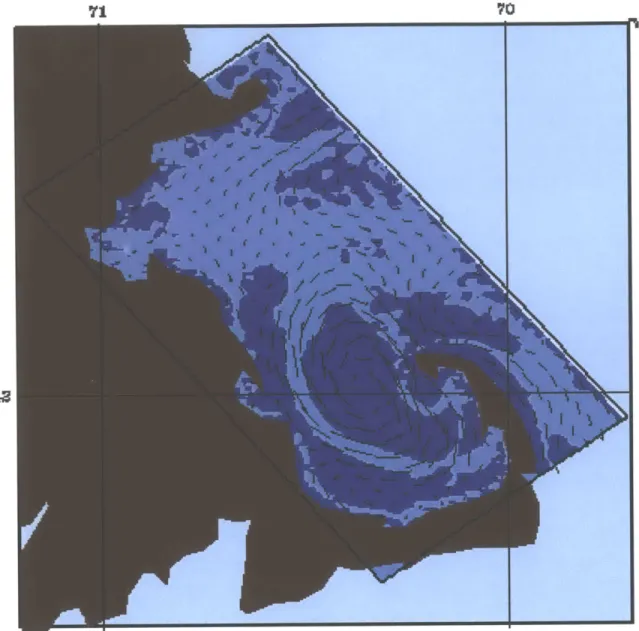
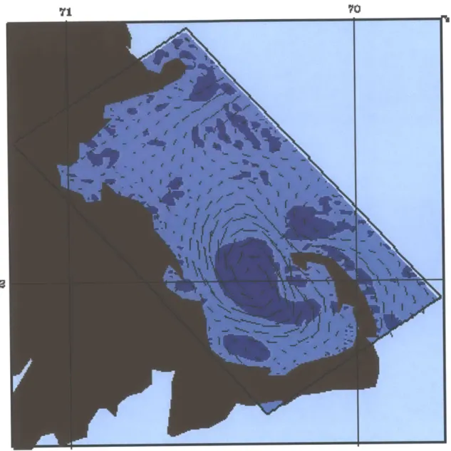
3-38 The result of the geometric method with the cleanup condition "A n (B U C)" in Massachusetts Bay. . . . . 98 3-39 The HOPS horizontal velocity magnitude and direction field in the

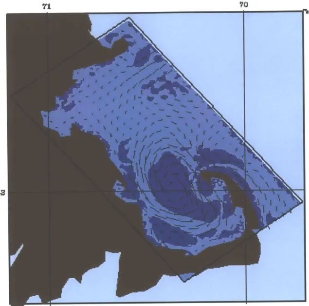
3-40 The Boolean values of the vorticity magnitude with the threshold of twice the mean of the vorticity field, with superposed velocity vectors in the Western Mediterranean. The deeper color denotes the vortex area. 102 3-41 The result of the conjugate pair eigenvalues method in the Western

Mediterranean. The deeper color shows the vortex area . . . . . 103

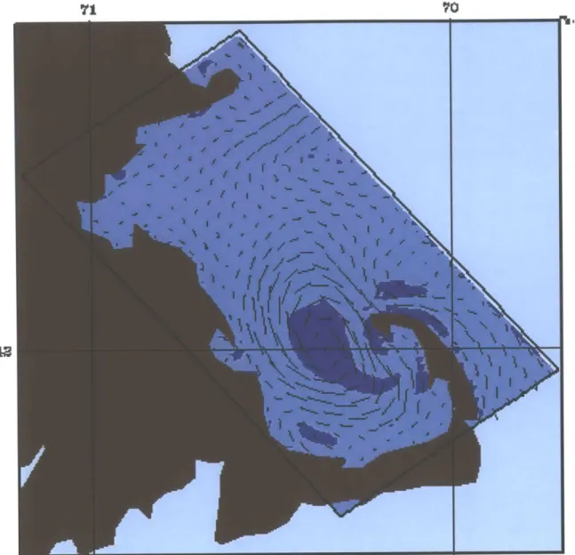
3-42 The result of the negative A2 method with superposed velocity in the

W estern M editerranean. . . . . 104 3-43 The result of the positive

Q

W estern M editerranean. . . . . 105

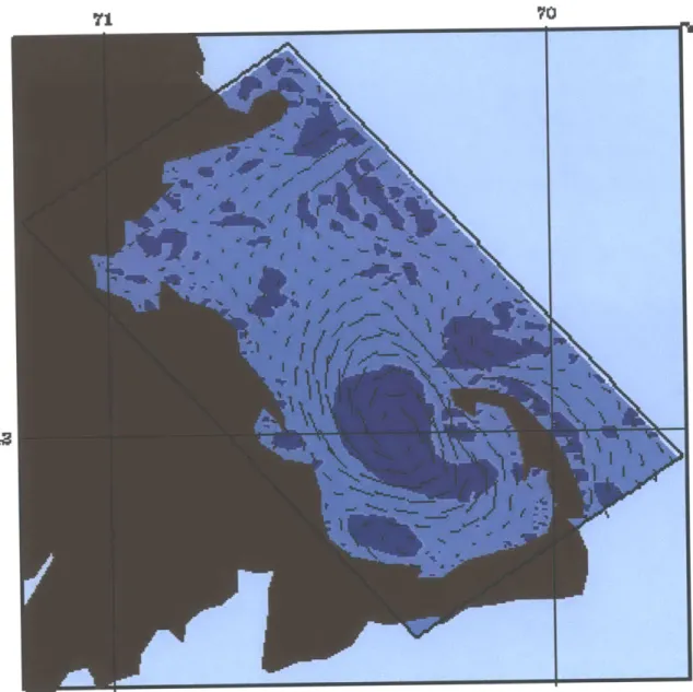
3-44 The result of the geometric method without cleanup in the Western M editerranean. . . . . 106

3-45 The result of the geometric method with cleanup in the Western Mediter-ranean. See next Figure for closeups of A, B, C and D. . . . . 107

3-46 The closeups of last Figure. . . . . 108

3-47 Inverse distance weighting . . . . 111 3-48 Transformation between P-space and C-space, adapted from [51.

.

3-50 A streamline approaching a limit cycle has to reenter cells, taken

from [61]. . . . . 116

3-51 If a real exit can be reached, the streamline will leave the cell cycle,

taken from [61]. . . . . 116

3-52 If no real exit can be reached, the streamline will approach a limit

cycle, taken from [61]. . . . . 117

3-53 In a vortex core, four axes can be drawn which are parallel to domain

boundaries. . . . . 119

3-54 Four possible situations of a streamline. . . . . 120

3-55 The streamline E could not "bypass" vortex core 0 if 0 is the only

vortex core in the region. . . . . 121

3-56 Streamline A is a closed streamline but streamline B is not . . . . . . 121

3-58 Upwelling in a confined vortex, taken from [3]. . . . . 123

3-59 Swirling plane and core direction in 3D vortex core region, adapted from [25]. . . . . 123

3-60 Quantization of range and axis. . . . . 124

3-61 The result of winding angle method in the Western Mediterranean. . 126 3-62 The result of the "cross" method in the Western Mediterranean. . . . 127

3-63 The result of the "cross" method in the Western Mediterranean. . . . 128

4-1 Coastal upwelling . . . . 134

4-2 Equator upwelling . . . . 135

4-3 Upwelling in Massachusetts Bay . . . . . 137

List of Tables

List of Symbols

VXY

VXY- horizontal divergence operator material derivative p pressure p density f Coriolis parameter T stress tensor V kinematic viscosity t time IF circulation v velocity vector

Vr radial (r) component of velocity

VO tangential (0) component of velocity

VZ vertical (z) component of velocity

h helicity

w vorticity

A eigenvalues

Vv velocity gradient tensor

J Jacobian (velocity gradient tensor)

S symmetric part of J

Q antisymmetric part of J

x _{position (x, y, z)}

Chapter 1

Introduction

1.1

Poseidon Project

Research on realistic nonlinear interdisciplinary processes has considerably expanded the knowledge of the complex coupled physics, biology and acoustics of the oceans. In order to effectively manage coastal marine resources and their impact on climate, powerful and sporadic biophysical events must be scientifically understood and pre-dicted. To achieve this end, ocean forecasting, a process involving biological, chemical and physical aspects, is needed [36].

Essential to ocean forecasting is the continual melding of new observations into predictive dynamical models, and such observations must be obtained at the right time and space in the episodic ocean, thus calling for adaptive sampling. In spite of effective omission and aggregation efforts, the physical, biological and acoustical state variables and parameters remain large in number; this necessitates the evolu-tion of the dynamical model parameters and structures during the predicevolu-tion through adaptive modelling. The objective of the Poseidon project is to achieve efficient mul-tiscale interdisciplinary ocean prediction with real-time objective adaptive sampling, assimilation of multiple streams of interdisciplinary data, and autonomous adaptive modelling through an effective union of information technology and ocean science.

Facilitated by the widely available, high-performance computing hardware, net-working infrastructure, tools and interfaces for access, it is possible to construct a

distributed ocean prediction computing system and using networked, scientific com-puting to effectively address a wide range of computationally intensive problems. The Poseidon project is developing an information system that can address the needs of interdisciplinary ocean scientists, making it possible to construct and execute complex domain-specific workflows in a simple and robust way.

The Poseidon project is based on a series of Observation System Simulation Ex-periments (OSSEs) with the Harvard Ocean Prediction System (HOPS) for three regions of the (near) coastal northwestern Atlantic which exhibit coastal upwelling, spring and tidal mixing plankton blooms, and the mesoscale eddy injection of nutri-ents into the upper ocean [36]. Acoustic tomographic data and acoustical and optical backscatter data are incorporated into the data streams for assimilation. As the sys-tem is developed and tested, the OSSEs are iterated from both ocean and information sciences approaches. The Poseidon project attempts to enhance scientific productiv-ity, cultivate a new generation of interdisciplinary researchers, and contribute to the prediction and monitoring of marine resources in the multiuse coastal waters.

1.2

Harvard Ocean Prediction System (HOPS)

The Harvard Ocean Prediction System (HOPS) is a system of integrated software for multidisciplinary oceanographic research [63] [1]. It is designed to provide:

" "the naval ocean forecaster with accurate estimates of ocean fields in

a timely and reliable manner";

* "the physical oceanography scientist with realistic simulations of the ocean in order to study fundamental dynamical mesoscale processes"; * "the acoustical oceanography scientist with tools to obtain reliable

representations of the mesoscale sound speed variability";

* "the bio-geochemical oceanography scientist with an integrated en-vironment to carry out coupled physical-bio-geochemical model sim-ulations".

HOPS is configured as a nowcast/forecast system and is designed to meet

ship-board operational needs requiring adaptability to diverse data streams and dominant physics in a given region. It is able to be exercised fully as a stand-alone system uti-lizing ship gathered information only. HOPS, a research and training tool for physical oceanography scientists, can facilitate the generation of physical fields suitable for pro-cess studies and allow efficient exploration and exploitation of new algorithms and ideas. The configuration of HOPS for interdisciplinary research serves as a laboratory for the investigation of the influence of the physical environment on the evolution of the oceanic bio-geochemical mass and sound propagation.

The distributed version of HOPS includes the software structured to work in an integrated fashion especially with regard to inputs and outputs. At the heart of HOPS is a primitive equation dynamical model supported by a series of routines, including data gridding routines, initialization and assimilation field preparation routines, vi-sualization software, data preparation codes and topography conditioning software. The overall system schematic is shown in Figure 1-1 on page 24.

1.2.1

Harvard Primitive Equation Model

Models included in the Harvard Dynamical Modelling System are a Primitive Equa-tion Model [52], a Quasi-Geostrophic Model [35] and a Surface Boundary Layer Model [58]. The emphasis here is placed on the the Harvard Primitive Equation Model for Coastal and Deep water, which is applicable to any oceanic region, with arbitrary coastline and/or open boundary segments. The GFDL (Geophysical Fluid Dynamics Laboratory) model offers the dynamical integration algorithm. The deep ocean version of the Harvard model was then developed by adding open boundary conditions, terrain following coordinates, and subgrid scale physics appropriate for mesoscale resolution [32].

HOPS can provide accurate computations in the deep ocean with steep topogra-phy, the shelf break and the shelf region.

Bryan [8] and Cox [12] both documented the GFDL algorithms, and Spall and Robinson [52] further expounded the details of the deep ocean model developments.

Harvard Ocean Prediction System

-

HOPS

TAS

Remotely Sensed and In

Situ

Real Time and Historical

SAdaptive

Database

Sampling

1

Penetrative

Heat Flux

Initialization,

Assimilation, &

Surface Forcing

FI

Transport

Processes

T

[Chl]

Surface Forcing

(Solar Insolation)

Init.

&

Acoustical

Dynamical Model

Init. &

Applications

Figure 1-1: System schematic of the HOPS. Chl, and PAR stand for chlorophyll, and Photosynthetically Active Radiation.

Physical

Dynamical

Model

I

Optical Dynamical

Model

Light Attenuation and Propogation

Biogeochemical/

,Ecosystem

Dynamical

Model

I

What follows is a description of recent developments. These and future developments are facilitated by modular codes managed under the UNIX source control system and code pre-processing options allowing for flexible support of diverse hardware platforms, physics and algorithm options.

Model Physics

According to [311, "the basis for the Primitive Equation Model is the Navier-Stokes equations in a rotating reference frame with the two main simplifying assumptions, appropriate for most deep ocean and shelf regions. One assumption is the Boussinesq approximation, which retains density variations only in the buoyancy terms. The other is the hydrostatic approximation. Further approximations based on dimen-sional analysis are included in the canonical primitive equations. In particular, the geopotentials are assumed to lie on concentric spheres; the gravitational field is taken to be constant throughout the domain; only the vertical component of the earth rota-tion vector is retained; the solid boundaries are assumed to be rigid and impermeable; and the heat and salt fluxes normal to the solid boundaries are assumed to be null.

In the future, a free surface option will be provided."

With these assumptions, the canonical primitive equations are [37]:

VXY - U+ w = 0 +

xiz

gp

at

where, Div is the three-dimensional divergence operator; V x- is the horizonal divergence operator; VxY is the horizontal gradient; ez is a unit vector in the vertical direction; 6/6t is the material derivative; U-, w the horizontal and vertical velocities; p is the pressure; p is the density;

f

for additional subgrid scale physics and qr, qs are the heat and salinity flux vectors.

1.2.2

Grid Types

Horizontal Coordinates

There are three types of horizontal domains currently supported by HOPS: Cartesian, spherical and rotated spherical (Figure 1-2 on page 28) [32] [63].

1. Cartesian: The Cartesian grids are local tangent plane approximations to a sphere, often used for a small regions where spherical effects are relatively unim-portant. The Cartesian transformation is defined by three parameters:

(late, lon,): The "center" of the transformation. Geographic coordinates are converted to Cartesian based on the distance to this point.

0rot: The rotation angle. The Cartesian coordinates, (xy), are rotated from

their geographic counterparts, (lat, Ion), by the angle rot.

The Cartesian domains are further defined with six additional parameters: (nx, ny): The number of grid points in each direction.

(dx, dy): The grid spacing in each direction.

(Ax, Ay): The offset (meters) between the center of the domain and the center of the transformation.

2. Spherical: The spherical grids are geographic latitudes/longitudes. They are often used where spherical effects are important and it is more convenient to keep geographic orientation. There is no transformation, so latc, lon, and 0rot are all zero. The domains are defined with six parameters:

(nx, ny): The number of grid points in each direction.

(dx, dy): The grid spacing in each direction.

(Ax, Ay): The offset (degrees) between the center of the domain and the center of the transformation. For the spherical grid, (Ax, Ay) become the (lat, lon) of the center of the grid.

3. Rotated Spherical: A spherical grid in which the equator had been moved to

reduce model grid distortions. It is often used for regions where spherical effects are important and reducing model grid distortions outweighs any benefit of maintaining geographic orientation. The rotated spherical transformation is defined by three parameters:

(latc, lon,): The "center" of the transformation, which is the (0,0) point of the

rotated spherical system.

Orot: The rotation angle. The angle between the rotated coordinates and the geographic coordinates at the "center" of the transformation.

The rotated spherical domains are defined with six additional parameters: (nx, ny): The number of grid points in each direction.

(dx, dy): The grid spacing in each direction.

(Ax, Ay) The offset (degrees) between the center of the domain and the center of the transformation.

Vertical Coordinates

There are three types of vertical domains currently supported by HOPS: o Coordi-nates, Hybrid Coordinates and Double c- Coordinates (as in Figure 1-3 on page 30).

1. - Coordinates: The depth of a model is a fixed fraction of the total water column.

Zi,j,k -- O- * hij (1.2)

The o coordinates are most useful in regions with high topography and where maintaining near surface resolution is not necessarily critical.

2. Hybrid Coordinates: A generalization of (1). The top k, levels are flat, the remainders are terrain that follows,

Northwest Atlantic, 30km (Cartesian) Friday - July 28, 2000 - 6:12:04 pm

Northwest Atlantic. 0.2r (spherical) Monday - July 31. 2000 - 1:27:37 pm

Northwevt AtaIUo. 0.27(rotated spherioil) Tuesday - August 1. 0000 - 1:08:06 pm

45N

40' N

55N

6 6 P9 PC6

Figure 1-2: Horizontal grids in HOPS: Cartesian, spherical and rotated spherical.

4(rN 40'N 35"N 40' N 40' N 55 N 6 C

Zijk = Zk (k

<

(1.3)

(hi

zc)

(k

kc)

Where z, is the depth of the flat interface between the two vertical coordinate systems and the convention 0 ok I 1 is used.

The hybrid coordinates are often used in deep ocean where maintaining near surface resolution is important.

3. Double - Coordinates: A generalization of (2). The constant coordinate inter-face, z., is replaced by one that varies in the horizontal to ride above topography. The variable coordinate interface,

fij~,

fj = CI+ ZC2 + ZC C2 tanh{

[hij -

2 2 zc1 - ZC2

Where,

zci: The shallow limit for the coordinate interface. zC2: The deep limit for the coordinate interface.

hre: The"switching" depth.

fij

a: The slope parameter. How fast f responds to changes in the topography, h.

Also a limit on the slope of

f,

||Vf||

a||Vh||.

The vertical system is: a o system referenced between the surface and

fij

fij

Zijk = Uk *fij

(k < kc)

(1.5)

fij + (Uk - 1) * (hij -

fi,j)

where, the (arbitrary) convention 0 Uk < 1 for k

<

with shallow topography and where it is important to maintain near surface resolution.

- 0 2 2 2 0 -500 -1000 -1500 -2000 -200 -3500 -00 (b) Schematic of Hybrid Sy -500 -Flat -1000---2000 -2500 -3000 -3500 -4000 -4500 0 20 40 60 80 100 120 Range (I-2) (d)

Schematic of Double Sigma System

C, G . ... .. ... .... |-- z G2 ctI~viII -80 100 0 20 40 60 Range (ln) 120 -500 1000 000 2500 3000 200-60 70 81 (c) M4W Aftdoi- 0Ibrid 0 10 20 30 40 D 60 70 00 (c) NOW- ---0 10 20 20 40 M0 s0 20 00 R-* OrnO

Figure 1-3: Vertical grids in HOPS: (a)Single a coordinates. (b-c) Hybrid coordinates. (d-e) Double - coordinates.

30 O 10 20 30 40 w -50 -100 -150 A-2500 -3000 -3500 -4000 -4500 1000 1500 2200 2500 3000 4000 450

T T T

x 1,

* 1... ...

T T Ti+J1

(a)

Figure 1-4: (a) Horizontal layout.

T i-1,+r -W i )+1 T I-1,k+2 (1) ) (b) Vertical layout.

An example of horizontal and vertical layout of a grid is as in Figure 1-4 on page 31. In horizontal layout, T stands for tracers (temperature, salinity, etc) and streamfunctions. U stands for both horizontal velocity components. In vertical layout, Tracer vertical boxes are shown, velocity vertical boxes have the same layout, merely shifted 1/2 grid space horizontally. W stands for vertical velocities.

In this paper we present our initial approach to vortex detection in ocean flows, applying 2D algorithms to the flow at multiple constant depths. Such methods, while less comprehensive compared to their 3D counterparts, allow us to efficiently identify horizontal structures in the ocean. Especially in the case of stratified ocean flows (which are more prevalent during the summer months) feature extraction in the horizontal dimensions can be very useful. As an added benefit, they are considerably less expensive and less sensitive to the vertical grid irregularities of most ocean models

than fully 3D algorithms.

1.3

Real Time Regional Forecasting

Being intermittent, eventful and episodic, the ocean is a turbulent fluid in essence and its circulation is characterized by a myriad of dynamic processes occurring over a

T T ]+1. z 7k

Tw

"'

_{Z L}

vast range of nonlinearly interacting scales both in time and space. Ocean forecasting allows us to effectively and efficiently manage operations on and within the sea. Such forecasting has been used for military operations as well as scientific research [41].

Forecasting usually starts with observations that can initialize dynamical forecast-ing models; further observations are then assimilated into the models as the forecasts progress in time. As a matter of fact, such observations are usually difficult, costly and incomprehensive. It goes without saying that if a region of the ocean were to be sampled uniformly over an arbitrary space-time grid, only a small subset of those observations would have significant impact on the accuracy of the forecasts. In con-trast, accurate forecasts target the intermittent energetic synoptic dynamical events and form the basis for designing a sampling scheme that can observe the ocean state. Adaptive sampling of features of greatest impact increases efficiency as it can reduce the observational requirements by several orders of magnitude.

The oceans evolve as time goes by, responding to both external surface and body forces, and internal dynamical processes. Some examples of external surface and body forces include tidal forces, winds and surface fluxes of heat and fresh water. Given the importance of air-sea interaction, ocean forecasts requires an accurate meteorological forecast. Analogous to atmospheric weather phenomena, ocean internal instabilities and resonances, including meanders of currents, fronts, eddies and wave propagation, are called the internal weather of the sea. Their spatial scales are short with respect to global scale, which requires the ocean forecasts to be carried out regionally as opposed to globally.

Furthermore, the regional forecast problem has additional forces appearing as fluxes through horizontal boundaries, a representation of both larger scales of direct forcing, remote internal dynamical events and land-sea interactions in the littoral zone. To develop a regional forecast system and capability, both the scales and processes of interest and the dominant scales and processes in the region are essential. Some of the fields of forecast interest are physical, acoustical, biological, optical, chemical and sedimentological state variables. Examples include velocities, temper-ature, sound speed, irradiance, plankton concentrations, scattering profiles and

sus-pended particle concentrations. Multi-disciplinary sampling schemes are constrained

by the interdisciplinary compatibility requirements. Some variables are of direct

in-terest whereas others are helpful in interdisciplinary field estimation such as the case of acoustic travel times in the estimation of temperature gradients. As a result, the scope of ocean forecasting has expanded, which in turn leads to rise of a challenging adaptive sampling problem, i.e., the design of sampling schemes for the acquisition of multi-scale compatible interdisciplinary data sets based on real time observations and realistic forecasts.

1.4

Adaptive Sampling

Adaptive sampling can help to collect the most useful data of an ocean field and help compute error forecasts through the use of quantitative criteria or goals. Cur-rent adaptive sampling methods [29] [44] [43] combine field and error forecasts with

a priori experience to intuitively choose the future sampling. This approach can conceptually be then automated: quantitative adaptive sampling utilizes forecasts as inputs to mathematical criteria whose real-time optimization produces the sampling pattern [42].

Current forecast capabilities involve the future evolution of ocean fields, of their variabilities and uncertainty statistics [28]. Various constraints remain, including practical considerations (platforms and sensors availability, ship speeds, autonomous underwater vehicle (AUV) range, weather conditions), dynamical motives (search for precursors of the primary phenomenon, dynamical model verifications), and cost penalties (fuel, batteries, labor costs). Moreover, scientific and technical constraints exist for the measurement model to generate the actual state variables to be assimi-lated. Finally, in varied representations, several goals or criteria are also a possibility. One type of optimum can be the sampling that minimizes the forecast of the field error variance confined by cost penalties and practical constraints. Others belong to the best skill evaluation samplings that perfectly define specific properties of future dynamics, independent of past data and other constraints. Assimilation studies also

use data assimilation criteria to develop the goal accordingly. Thus, the assimilation study aiming at minimizing the field error with a variance metric would set the adap-tive sampling goal as determining the future sampling that minimizes the trace of the error covariance matrix.

For linear models, the optimization can be implemented independent of future data values, making use of the dynamical and measurement models and their uncertainties. For non-linear models, data values make a difference and a forecast OSSE needs to be done during the optimization process. Research on optimal control and estimation theory can be applied and extended by interdisciplinary oceanographers to obtain the

most useful sampling methods.

The process of feature extraction discussed in this thesis facilitates user-assisted adaptive sampling and could eventually be used to help automate this optimization procedure.

1.5

Problem Statement

Given the vastness of ocean, it is essential for effective ocean prediction to employ adaptive sampling to best utilize the available sensor resources in order to minimize the forecast error. It is important to concentrate measurements to the regions where one can witness features of physical or biological significance in progress. Thus, automated feature extraction in oceanographic visualization can facilitate adaptive sampling by presenting the physically relevant features directly to the operation plan-ners. Moreover it could be used to help automate adaptive sampling. Therefore, the study of automated feature extraction in oceanographic visualization is introduced.

A series of Observation System Simulation Experiments (OSSEs) with the Harvard Ocean Prediction System (HOPS) provide the basis, the large-scale HOPS datasets in different ocean regions, for this study. The task is to detect typical oceanographic features from these large-scale datasets.

Vortices (eddies and gyres) and upwelling, two typical and important features of the ocean, are studied. A variety of feature extraction methods are presented, and

those more pertinent to this study are implemented, including derived field generation and attribute set extraction. Detection results are evaluated in terms of accuracy, computational efficiency, clarity and usability.

Vortices, a very important flow feature is the primary focus of this study. Several point-based and set-based vortex detection methods are reviewed. A set-based vortex core detection method based on geometric properties of vortices is applied to both classical vortex models and real ocean models. The direction spanning property, which is a geometric property, guides the detection of all the vortex core candidates, and the conjugate pair eigenvalue method is responsible for filtering out the false positives from the candidate set. Detection methods of streamlines are also discussed. Using the novel cross method or winding angle method, closed streamlines around vortex cores can be detected. Therefore, the entire vortex area, i.e., the combination of vortex core and surrounding streamlines, is detected. Accuracy and feasibility are achieved through automated vortex detection requiring no human inspection.

The detection of upwelling using integration methods is also discussed.

1.6

Thesis Outline

The organization of this thesis is as follows.

* Chapter 2 provides an overview of feature extraction and scientific visualization techniques.

" Chapter 3 discuss vortex detection. First, different vortex models are presented.

Second, the point-based vortex detection methods and set-based vortex detec-tion methods are reviewed. Finally, a geometric-based vortex core detecdetec-tion method and a novel "cross" method to detect closed streamlines are introduced.

" Chapter 4 describes upwelling detection.

Chapter 2

Feature Extraction and

Visualization

2.1

Feature Extraction

Features are regions of interest in a data set, be it a single grid location or a set of nodes from the data set. There are several methods available to extract the feature-sets from the data feature-sets. For example, in the area of vortex identification, there are two categories of algorithms, point-based and set-based methods, which will be discussed later. The means of feature extraction are feature criteria, which depend on the scientific domain as well as the specific features of interest. For example, it could be a Boolean criterion function, consisting of a logical combination of scalar thresholds, applied to data values or to derived data values such as velocity gradients [53] [57].

Attribute sets are defined as sets of characteristic values computed from the ex-tracted features in the data set. They can involve a combination of scalars, tensors and vectors. When a feature goes beyond a single grid position or cell, relevant attributes including volume, mean data value, center and various moments can be obtained by using volume integrals to do an integration over this region. Attributes fall into two categories, either purely geometric or involving a combination of geometry and the underlying data values.

steps required to identify these regions:

1. Find the nodes which meet certain threshold criteria. 2. Partition the nodes into connected regions.

3. Extract the bounding surface of each connected region.

2.1.1

Oceanographic Features

There are many oceanographic features in the ocean, such as upwelling, fronts, jets/meanders, vortices, geostrophic turbulence etc. These oceanographic features are caused by combined rotation and stratification effects. For instance, coastal upwelling is a phenomenon resulting from wind forcing, Ekman dynamics and geostrophy [13]. A front is a relatively narrow region of intensified gradients of fluid properties between two main fluid masses. Under the action of Coriolis forces, the process of geostrophic adjustment is at work, leading to a relatively intense flow aligned with the front. The much weaker density gradients in the main part of each fluid mass confine the motion to the frontal region, and the flow exhibits the form of a jet. The jet has a velocity maximum, coinciding more or less with the location of the maximum density gradient, on both sides of which the velocity decays. Meanders and shed vortices can also exist in a jet area. Meanders on a jet do not remain stationary but propagate, usually downstream and rarely upstream. A vortex, or eddy, is defined as a closed circulation that is relatively persistent, which means that the turnaround time of a fluid particle embedded in the structure is shorter than the time during which the structure remains identifiable. When several eddies are present and are not too distant from each other, interactions are inevitable. Vortices shear and peel off the sides of their neighbors and, at times, merge to create larger vortices. The sheared elements either curl onto themselves, forming new, smaller vortices, or dissipate under the action of viscosity. The net result is a combination of consolidation and destruction. The state of many interacting vortices under the influence of Coriolis effects is geostrophic turbulence.

Research in detecting these features would help understanding the complex cou-pled physics, biology and acoustics of the oceans and could be used to help automate adaptive sampling.

2.2

Scientific Visualization

Visualization literally means making things visible. In general, it is concerned with providing visual images to understand something that can not be directly seen under normal circumstances. In the context of this paper, the meaning of visualization is confined to the visualization of data stored in a computer, the goal of which is to ex-plore and understand data sets. As a subcategory of computer graphics, visualization refers to algorithms, programs, techniques and systems that produce images.

A review of the field of visualization in computer graphics can be found in [34]. Visualization could again be divided into two sub-fields - information visualization and scientific visualization. Information visualization deals with discrete data often with high dimensionality and depicts properties of a large but finite number of data items. Scientific visualization, on the other hand, is good at handling continuous data often with low dimensionality. Such data represents a continuous field, though in practice it is usually sampled on a discrete set of locations. The two subfields

sometimes merge.

2.2.1

Volume Visualization Techniques

There are a great variety of volume visualization techniques able to probe 3D fields, and they differ on the type of field being investigated, be it a scalar, vector or tensor, and the type of information sought. Isosurface and volume rendering are two major 3D visualization methods to explore scalar volume datasets.

Isosurface

An isosurface is defined as a surface of a constant threshold within the dataset and contains points where p(x, y, z) = a for a particular threshold value a. To

approxi-mate an isosurface, polygonal primitives such as triangles can be generated by surface fitting algorithms and then projected onto a 2D display.

As the most frequently seen isosurface technique, the marching cubes algorithm [30]

constructs a contour surface for every cell in the volume. A case table is set up that enumerates all possible topological states of a cell, taking consideration of combina-tions of scalar values at the cell vertices. The number of topological states relies on the number of cell vertices, and the number of vertex-to-contour value relationships. When the vertex's scalar value is larger than that of the contour line, the vertex is considered within the isosurface. In the same vein, vertices with scalar values lower than the contour value are defined to be outside the isosurface. The resulting binary encoding creates indices for a case table, which denote how the contour intersects the cell. The algorithm marches through the volume one cell after another, and linear in-terpolations are used to calculate the isosurface locations. The isosurface is complete after all the cells are visited. Since the marching cube algorithm tends to produce a large number of triangles, a triangle decimation algorithm is useful in reducing this number.

Volume Rendering

An isosurface is only a partial representation of the dataset. For a complete view of

3D data, a class of techniques known as volume rendering offers an inside picture of

the data. Volume rendering refers to an approximate simulation of the propagation of light through a participating medium represented by the volume. In comparison to the traditional surface rendering techniques, this offers a more effective way to convey information within volumetric data as it can project the entire 3D volume directly onto a 2D plane.

Object-order and image-order are two basic approaches of volume rendering [17]. The former uses a forward mapping scheme to project voxels onto the image plane whereas the latter uses a backward mapping where rays are cast from each pixel in the image plane through the volume to determine the pixel color results. Some researchers have also combined the two techniques. Volume rendering algorithms

involve a transfer function to blend or composite data onto a 2D image plane. This transfer function has to be chosen with deliberation to be able to offer segmentation and generate surface like objects. The vector and tensor fields can be visualized by a set of arrows, other point icons or glyphs, which is discussed in detail in [46] [62].

2.2.2

Scientific Dataset Format

The HOPS data are stored in the NetCDF format [1]. The Network Common Data Form, or NetCDF, is an interface to a library of data access programs for storing and retrieving scientific data [4]. NetCDF is an abstraction that supports a view of data as a collection of self-describing, network-transparent objects that can be accessed through a simple interface. Collections of named multidimensional variables can be randomly accessed, without knowing details of how the data are stored. Auxiliary information about the data, such as what units are used, can be stored with the data. Generic utilities and application programs have been written that access arbitrary NetCDF files and transform, combine, analyze, or display specified fields of the data. The development of such applications was led to improved accessibility of data and reusability of software for scientific data management, analysis, and display. The NetCDF interface is supported for the C, FORTRAN and Java computer languages, and for UNIX and Windows operating systems. A NetCDF file has dimensions,

variables, and attributes. These components can be used together to capture the

meaning of data and relations among data fields in a scientific data set. A NetCDF file is constructed as:

netCDF name

{

}

NetCDF dimension declarations appear after the dimensions keyword, NetCDF variables and attributes are defined after the variables keyword, and variable data

assignments appear after the data keyword.

Data can be categorized into scalars, vectors, and tensors. Scalar data is a magnitude without a direction, for example, temperature, salinity, density, transport streamfunction, etc. Vector data consists of magnitude and directions, which are usually represented as an n-tuple, where n is the dimension of the space. In 3D, it is represented as a triplet of values (x,y,z). Total velocity, geostrophic velocity and vorticity are examples of vectors. Tensors are complex mathematical generalizations of scalars, vectors and matrices. A tensor of rank 0 is a scalar, rank 1 a vector, rank 2 a matrix, and a tensor of rank 3 is a three-dimensional rectangular array. Tensors of higher rank are k-dimensional rectangular arrays. Stress and strain are examples of symmetric tensors. However, in HOPS NetCDF data files, there is no tensor field available.

In HOPS, datasets are sampled on 3D grids. In general, grids are organized to resemble the actual geometry under approximation. The space where the physical phenomena are defined is referred to as the physical space, where data are sampled on the grid nodes and stored in discrete forms of numerical values. On the other hand, in computational space, data are organized into a rectangular uniform mesh in a logical order to ease numerical computation. Between the two spaces, mapping in both directions must be done. Numerical computations performed in the computational space generate results that are mapped back into the physical space for visualization purposes.

2.2.3

Visualization Pipeline

The process of obtaining an image from a data set can be roughly classified as four stages. The final image is achieved through four stages of operations on the original data. The first stage is data input during which a data set is read in or generated, resulting in the original field data in the form of a grid. The second stage is filtering, where several filters may be applied on the data. Both the input and output is a grid in most cases. The third stage is mapping during which the grid data is transformed into geometrical primitives. In this key visualization step, the data are converted into

a collection of triangles, lines, points or icons. The final stage is rendering, where an image is finally generated by rendering the geometrical primitives according to a particular computer graphics model.

Most algorithms targeted at scientific visualization are associated with the map-ping stage. Marching Cubes [301, an approximation of an iso-surface, is the most prominent visualization algorithm. Other commonly used visualization techniques include scatter plots, contour plots, arrow plots, height field representation and di-rect volume rendering techniques [14].

2.2.4

HOPS Visualization Pipeline

Visualization in HOPS is achieved in the HOPS Plotting Package [1]. The HOPS data

are stored in NetCDF format. In addition, an input script .in file which includes plotting commands, the parameters input file, the color palette input file and the contour parameters input file are also needed in order to get visualization results. The plotting package has five executable programs:

" cnt-ncar: horizontal contours, non-color version.

input script: pe-cnt.in or qg-cnt.in

" ccnt-ncar: horizontal contours, color version.

input script:pe-ccnt.in or qg-ccnt.in

* ccntmd-ncar: horizontal contours, color version, multiple domains'. input script: ccntmd-ncar.in

" sec-ncar: cross-section contours, non-color version.

input script: pe-sec.in or qg-sec.in

* csec-ncar: cross-section contours, color version. input script: pe-csec.in or qg-csec.in 'HOPS can handle nested domains.

The prefixes "pe" and "qg" in these script file names indicate the type of field classification used: either PE (Primitive Equation) or QG (Quasi-Geostrophic) field identifiers.

The data fields in all "horizontal" levels (discrete constant --value isosurfaces) in a HOPS data file can be visualized. The data fields at an actual depth, which are interpolated from existing levels, can also be visualized. Nowcasts and forecasts can be obtained.

The filtering is done by HOPS Fortran 77 routines and our newly developed feature extraction Fortran 77 routines. Feature extraction routines are specialized in detect-ing features of interest. For instance, in vortex detection, the whole algorithm which includes several filters would be applied to the total velocity field. With the help of

NCAR Graphics Library [3], basic and advanced visualization can be achieved. The

plotting package uses NCAR Graphics' GKS [1] [3] utilities to help accomplish

map-ping and rendering, that is, the HOPS Fortran routines call corresponding NCAR's Fortran subroutines to convert data into a collection of lines, points or icons. Some visualization techniques, such as contours, iso-surface and volume rendering, are also easily done by calling NCAR's routines. Therefore, scalar fields and vector fields in

HOPS data files can be properly visualized.

NCAR Graphics Library

The NCAR Graphics Library [3] is a Fortran and C based software package for sci-entific visualization which contains a large number of Fortran/C utilities for draw-ing contours, maps, vectors, streamlines, weather maps, surfaces, histograms, X/Y plots, annotations, etc. It enables users to apply advanced visualization and analysis techniques to their data. These techniques can be applied to help users gain new insights into data from applications in a wide variety of fields. The NCAR graphics is discipline-independent and easily adapts to new applications and data.

2.2.5

Feature-Based Visualization

Research on feature-based visualization focuses on providing feasible visualization techniques that are semi-automatic and require less user time and little a-priori knowl-edge of the feature locations. A feature is defined in this context as anything contained in the data set that might be of interest to the user. A feature-based data represen-tation is a high-level data description able to replace the original represenrepresen-tation in a succinct and meaningful manner [46].

Less complexity, more information content and a good match to the concepts of the application area, are some of the goals of feature-based methods. By focusing on the user-defined effects or events, feature-based visualization is intended to improve the efficiency of the visualization process. Apart from the normal visualization pipeline, feature-based visualization adds on an automated analysis performed directly on the data set in question and able to get a set of features that are typically represented as icons at the location of the feature.

The demand for feature-based techniques has been growing with increasing avail-ability of simulation data sets. In fluid dynamics, for example, the size of data sets exploded with the wider adoption of time-dependent simulations, which reflected an increase in the resulting data of several orders of magnitude over a steady simula-tion. So far, only a few research groups have been actively engaging in feature-based visualization research [46] [18] [38] [40] [61] [64].

Examples of a feature-based techniques in oceanography are the extraction of eddies/gyres (vortices), upwelling and jets from real ocean fields. For visualization purposes, these features can be represented by different lines and icons either alone or combined with classical visualization methods. Features can also serve as guides to classical visualization techniques, an example of which is the placement of streamline seed points close to a vortex core. Moreover, the high-level data description of the features can be used for selective visualization. For example, a user can pick a set of features to be visualized instead of displaying all features found in the data set. The representation of point and line features does not require many graphic primitives,