HAL Id: halshs-00187885
https://halshs.archives-ouvertes.fr/halshs-00187885v2
Submitted on 16 Dec 2009
HAL is a multi-disciplinary open access archive for the deposit and dissemination of sci-entific research documents, whether they are
pub-L’archive ouverte pluridisciplinaire HAL, est destinée au dépôt et à la diffusion de documents scientifiques de niveau recherche, publiés ou non,
Chaos in economics and finance
Dominique Guegan
To cite this version:
Documents de Travail du
Centre d’Economie de la Sorbonne
Chaos in Economics and Finance
Dominique GUEGAN
2007.54
Chaos in Economics and Finance
Guégan D.
∗January 29, 2009
Abstract: This paper focuses on the use of dynamical chaotic systems in Economics and Finance. In these fields, researchers employ different methods from those taken by mathematicians and physicists. We discuss this point. Then, we present statistical tools and problems which are innovative and can be useful in practice to detect the existence of chaotic behavior inside real data sets.
Keywords: Chaos - Deterministic dynamical system - Economics - Estima-tion theory - Finance - Forecasting.
1
Introduction
Chaotic systems are complex systems which belong to the class of determin-istic dynamical systems. They are detected and used in a lot of fields for control or forecasting. Deterministic chaos has been rigorously and exten-sively studied by mathematicians and other scientists. It is almost impossible to give a precise mathematical definition of deterministic chaos that encapsu-lates everything in the diverse literature. In this paper we are not interested by complete mathematical rigour, and avoid technical details. Our viewpoint is to understand how the notion of chaotic systems is viewed, analysed and used in different fields.
As a first insight, we know that these systems are characterized by strong non-linearity, permitting to take into account non-periodic fluctuations, mixing
∗PSE, University Paris1 Panthéon -Sorbonne, CES-MSE, 106 Bd de l’hopital, 75013,
Paris, France, e-mail : dguegan@univ-paris1.fr, talk prepared for the 11Chaos’06 Confer-ence in Reims, June 28th - 30th June, 2006
cycles and switches inside data sets. They are characterized by an invariant distribution function and their orbits evolve inside an attractor in which it is possible to do forecasts. Working inside an attractor also permits to control the system and to be able to avoid explosions and strong volatility, which is an interesting task for applications.
Historically, mathematicians were the first to be interested by this theory. Since 1800, work concerning deterministic dynamical systems which gener-ate random behaviors has been investiggener-ated, and Poincare’s works (Poincaré, 1908) enable those studies to foster a growing interest and to be developed in a lot of communities. In biology, people who study population evolution have used chaotic deterministic systems since the 1970s, May (1976). In physics, it is a long tradition for researchers, working mainly with an empirical ap-proach, to use these models. The works of Ruelle and Takens (1971) proposed a new approach to non-linear modelling with few parameters and also gave the opportunity to extend the research in this field in this community. In economics, people working on stability and instability have flirted with bifur-cation theory since the 1980s. This approach is really new and unexpected coming from this community. Indeed, working with chaotic systems is in opposition to most of the different concepts developed by macro-economists: we cite for instance, the neo-classical theory of Lucas, Sargent, Prescott, etc, the ‘rational’ theory which uses mainly linear concepts or, Keynes’ theory which is not concerned with complex systems, Medio (1992). Between the years 1986 and 1998, a lot of studies, following the idea of Grandmont (1988), guided a part of the research in economics towards chaotic systems. In partic-ular, it explained randomness endogenously. New econometric models were developed and time irreversibility was introduced. In finance the interest in chaos theory is more recent and sparse. The craze for this theory from financial people began around the nineties. People expected to get robust forecasts using chaos. Finally, chaos has been recently developed as an area of increasing interest for statisticians.
Why are some statisticians so interested by the vast potential which can be gained studying deterministic chaos? One reason is that deterministic dynamical systems can generate chaos, that is highly erratic behavior remi-niscent of realisations of random process. Now, in the study of deterministic dynamical systems, environmental noise tends to be suppressed or, at most, plays a secondary role. In statistics, randomness is generated through a stochastic process and we speak about stochastic dynamical systems. What is the link between the deterministic characteristics of a chaotic system free of noise and the property of stochasticity? We can illustrate this fact using
the logistic map, largely studied in the literature, May (1976). Consider the following map defined by
Xt= 4Xt−1(1 − Xt−1), t = 1, 2, ... (1)
The solution of the logistic map, given a starting value, is also called a tra-jectory. If the starting value is between 0 and 1, then all the iterates of the logistic map will remain in the interval [0, 1]. The natural measure whose density is φ(x) = 1
π√x(1−x), 0 ≤ x ≤ 1, and zero elsewhere, reflects the fact
that each point inside [0, 1] will be visited arbitrarely closely and infinitely often. This natural measure is associated with a typical trajectory of the pre-vious logistic map and describes the ‘frequency’ of any point to be visited by such a trajectory and it can be linked with the marginal distribution of the lo-gistic map. Thus, we may introduce stochasticity into the lolo-gistic dynamical system by specifying the initial condition according to some probability dis-tribution. Then Xt, t= 1, 2, · · · , defined by (1), becomes a random sequence.
It is this link between the notion of chaos and stochastic environment which has been investigated by some statisticians, permitting to offer in real data analysis the possibility to extracting ‘chaotic’ signals from noisy data sets. Now, on the other hand, we can remark that, concerning the use of determin-istic chaotic systems, each community may have different strategies. They do not use the same models, nor the same information set. Most math-ematicians work with analytical expressions and characterize their models under specific assumptions to decide if they can exhibit specific chaotic be-haviors, characterized by specific properties, following varied definitions of ‘chaos’. The economists generally use analytical systems corresponding to a specific modelling problem. These systems depend on few parameters and one purpose is to detect the range of these parameters in which they can lead to stable or unstable behaviors. Bifurcation theory is often a basis of their studies. Generally economists do not follow the roads of physicists. In-deed, physicists are interested by questions relative to universal laws, and in economics the trend is to understand and document differences. In finance, practitioners do not use analytical systems and want to use chaos theory to robustify their forecasts: most of the work is empirical. In statisitics, work concerns estimation theory and tries to prove robustness of estimates of the Lyapunov exponents or the embedding dimension, for instance. They are aslo interested in re-building orbits and forecasting on the attractors.
2
What kind of chaos for which models?
Let Xt be a random vector characterized by the following equation
Xt= f (Xt−1), (2) and X0 an initial condition. The sequence (Xt)t corresponds to a dynamical
deterministic system and we assume that it is characterized by an invariant measure. This system is defined on a metric space A ∈ Rd
, d ∈ N and f is a non-linear function: A → A. As a working definition for our purpose, we will say that such a system has chaotic behavior if it is non-linear, if it is characterized by the existence of an attractor inside A and if it is sensitive to initial conditions (which means that there exists almost one positive Lya-punov exponent). Such a dynamical system gives rise to observations that have the characteristics of random data, and yet nevertheless are determin-istically generated. Throughout this paper we remain with this definition which is sufficient to explain the attemps of the different communities with respect to the chaotic theory. For more details on the notion of chaos, attrac-tors, and sensitivity to initial conditions, we refer to Devaney (1989), Katok and Hasselblatt (1995) and Guégan (2003), among others.
It appears very interesting to use chaos for modelling. Indeed, it is a non-explosive system (no trend); it is an aperiodic system (no seasonality); it is a stationary system (invariant distribution - ergodicity). Thus, if we are able to know in which space the attractor lies, by determining the phase space using the embedding dimension for instance, and if we are able to re-build the orbits, then we can make predictions.
1. Maps on [0, 1]. There exists a class of chaotic systems which has been developed, mainly by the mathematicians, and which gives simple ex-amples (toys) illustrating this theory. They are the maps defined on [0, 1]. They include the logistic map, the tent map and its generaliza-tion, the binary maps, etc., Guégan and Ladoucette (2002). Neverthe-less, while the logistic map found applications in biology and ecology, most of these maps are not very interesting for applications.
2. Chaos in experimental sciences. Chaotic dynamics have been observed in a wide variety of experiments, such as chemistry, physics, meterology, hydrology, medicine and biology, Lorenz (1963), Schaffer (1985) and Greenfeld (1992), for instance. Some of these studies are famous and illustrate the theory. They concern the detection of attractors, and bifurcation theory with computation of Lyapunov exponents. These
works are based on very well known chaotic systems such the Hénon, Lorenz, Rossler, Chua and Mackey Glass systems. These models, for instance, explain the behavior of resistance in physics, the water level of a river in hydrology, population growth in ecology, fish flux in fishing research or temperature evolution, Bergé, Pommeau and Vidal (1984). 3. Chaos in social sciences. The analysis of the behavior of individuals (auto-organization - reproduction) depends also on complex models, "closed" models, and researchers are interested to know their asymp-totic behavior. If we consider, for instance, the organization of a market looking at social behavior, it is assumed, in equilibrium theory, that the agents have complete knowledge of the market. But in fact, any agent has incomplete knowledge of the market. This knowledge comes from empirical observations, from which the agents learn, and then take some decisions. It appears that the information setting is not com-plete. Auto-regulation can be interpreted in terms of an attractor, but no known chaotic analytical model corresponds a priori to this fact. Nevertheless, this idea has been developed in the social sciences based mainly on behavioral surveys.
4. Chaos in economics. Macro-economists have long realized that a cer-tain class of deterministic non-linear sytems was capable of producing a self-sustained fluctuation without any shock from outside of the mod-els. A group of researchers including Benhabib and Nishimura (1979), Day (1982) and Grandmont (1988), for instance, have developed many examples of deterministic economic models that could generate non-periodic fluctuations. In a recent work, Brock and Hommes (1998) show that routes to chaos can arise in the traditional expectation models such as the cobweb model, and the asset pricing model by the introduction of heterogeneous beliefs.
5. Chaos in finance. In finance, some models try to explain the behavior of the chartists and the fundamentalists in a market through the evolution of exchange rates. One of these models follows the expression:
St= XtSt−1α S β
t−2, (3)
where Strepresents the exchange rate at time t and Xtsome behavioral
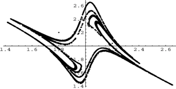
variable, α and β being the parameters of the system. For a specific range of these parameters, they have an attractor as given in Figure 1, de Grauwe, Dewatcher and Embrechts (1993). This work has proved that some models used in economics may produce either stable solutions
or complex solutions including a ‘chaotic’ solution. Following these ideas, an active research program has focused on evidence of chaos as the source of business cycles, Shintani and Linton (2004). In the same way, work has been developed to understand the dynamics of the labour market, or agents’ behavior in markets, using stock prices and currency exchange rates, although the detection of attractors empirically appears difficult because of the presence of measurement noise, Guégan and Mercier (1998). In another way, in order to make forecasts with data sets whose dynamics appear complex, detection of attractors have been considered after deconvolution using wavelets. As example, in Figure 2, we provide the attractor corresponding to the evolution of deconvoluted hourly electricity spot prices, Guégan and Hoummyia (2005).
1.4 1.6 1.8 2.2 2.4 2.6 1.4 1.6 1.8 2.2 2.4 2.6
Figure 1: Representation of the attractor of the system (3). On the vertical axis, we
represent Stand on the horizontal axis St−1.
0 5 10 15 20 25 30 35 10 15 20 25 30 35
Figure 2: Attractor for electricity German spot prices (Pt): Hourly prices from 16th
of June, 2000 to the 16th of December, 2004. Pt on the vertical axis and Pt−1 on the
horizontal axis.
Now, in practice, we observe only a trajectory X1,· · · , Xn that we assume
not sufficient to observe the auto-regulation or the reproduction of specific behaviors which can exist in the data. One way is to detect an attractor which could solve this problem.
How can we know that some attractor exists? Theoretically we have some answers. From two initial conditions, we can observe the divergence of tra-jectories and compute a positive Lyapunov exponent λ; we can consider a bifurcation diagram using the different values of the parameters of a model; we can make evidence of the attractor in the phase space of dimension d; we can compute its fractal dimension dH, d ≥ 2dH + 1. But, from a unique
trajectory (that is the case in economics and finance), we cannot use most of these techniques in practice. Indeed, bifurcation theory is not available be-cause we have only one experiment. The computation of dH is generally very
complicated. In return, we can estimate the Lyapunov exponents and test their positivity or we can investigate the attractor by successive embeddings. Thus, we have two choices: to work with an analytical system known a pri-ori, or to work with a time series without knowledge of analytical systems. The strategies need different knowledge.
• If we know the analytical system, we can estimate its parameters and build a bifurcation diagram. This approach is mainly used in control theory. It can detect existence of instability corresponding to chaotic behavior. Researchers, mainly dynamicists and economists, obtain the range of the parameters corresponding to the stable and unstable pe-riods.
• If we do not want to use a specific model, we need to embed the time series in order to detect the attractor - if it exists. We obtain it using Takens’ (1996) approach, building, from observations, for a certain d ∈ N and τ ∈ R, the orbits (Xt, Xt−τ, Xt−2τ,· · · , Xt−dτ), then we work
using the re-built attractor. This approach is employed by statisticians, practitioners in finance, insurance and economics researchers.
In both cases estimation theory is helpful. The embedding technique provides an estimate for d. Then, in the phase space, we can estimate the Lyapunov exponent λ, Wolff (1992), Bayley (1998), Guégan and Leroux (2009a) and test its positivity. In all procedures, we need to reconstruct the chaotic fun-tion f using non-parametric methods. Finally, forecasts can be provided. On the other hand, we know that random behavior does not create chaos: this is the case for noisy economic data sets or noisy financial data sets
(no attractor appears in the successive embeddings) and, we know that an ordered behavior does not fill the space providing an attractor. It is this last property that is useful in time series modelling. Thus, to be free of the presence of noise is fundamental in applications. If we want to suppress it, we need to work by deconvolution: see Dechert and Gençay (1992) and references therein and, Guégan and Hoummiya (2005) for recent developments using wavelets techniques.
3
Statistical tools for chaos theory
In this section, we specify the statistical tools which support the attemps of practitioners in economics and finance when no model is known a priori. We do not enter into details, and refer to basic works. Estimation theory is important and also the predictive approach, thus we discuss these two facts. As we already said, the observation of one trajectory X1,· · · , Xn cannot
detect the existence of an attractor characterizing the data set (Xt)t. The
embedding of the data set is then necessary.
• In a first step, we need to estimate the embedding dimension d. This estimate ˆd is obtained using non-parametric techniques: The delay method (Takens, 1981), the Grassberger and Procaccia method (1986) or the zero-one explosive method, Bosq and Guégan (2003), see Guégan (2003) for a review. As soon as we have found the smallest embedding dimension, if the attractor exists, it is evident from the orbits of the system corresponding to the data set (Xt)t=1,··· ,n.
• Second, we estimate the Lyapunov exponents and test their positivity in order to provide a measure of the chaoticity of the data sets. If we assume that the random variables (Xt)t=1,··· ,n are characterized by
the dynamical system defined by the map (2) which is assumed to be ergodic, then the Lyapunov exponent can be computed as follows:
ˆ λ= lim n→∞ 1 n n−1 X t=1 ln | ˆf′ (Xt)|,
when this limit exists and if the chaotic map f is differentiable, Wolff (1992), Delecroix, Guégan and Léorat (1997). The Xtare the points of the orbits built from an initial condition X0. The Shintani and Linton test (2004) can then be used.
• Third, the computation of ˆλ necessitates the knowledge of ˆf and of its derivatives. To solve this problem we use non-parametric techniques: nearest neighbors, radial basis functions, neural networks or kernels, we refer to Pesaran and Potter (1993), Guégan (2003) and references therein.
Considering the time series, we can decide to characterize them through an anlytical model known a priori. In that case, classical estimation theory developed for stochastic dynamical models can be applied, such as the least squares method. These techniques will be used in economics when we search a specific range of values for the parameters to detect stable and unstable periods in order to apply control, for instance.
In finance, generally, we only observe one trajectory of a time series and the purpose of the study concerns predictions using this information set: short, medium and long term predictions. As soon as the function f is well re-built, short term predictions on the attractor can be computed easily. To get medium term or long term predictions is always an open problem. Tradi-tionally, working with chaos means the inability to make forecasts, in return, working with ‘stochastic’ processes permits to compute forecasts. In that last case, if the model has short memory behavior, we make short term pre-dictions. If the model has long memory behavior we will be able to make long term predictions. A process is said to have short memory behavior if its autocorrelation function decreases with an exponential rate towards zero; it has long memory behavior if its autocorrelation function decreases with an hyperbolic rate towards zero, Guégan (2005).
Now, coming back to our discussion introduced previously concerning the property of chaoticity of some deterministic dynamical systems, it will be interesting, for such chaos, to investigate its behavior in terms of short or long term memory. For instance, chaos may have the same behavior as white noise (in terms of the behavior of its autocorrelation function): it is the case of the logistic map. In that latter case, it is not possible to make more than short-term predictions. To get these predictors, we compute iteratively
ˆ
fn(Xn), ˆfn(Xn+1), · · · , ˆfn(Xn+h). Examples of short term predictions using
financial data sets are provided in Guégan and Mercier (2005).
It will be interesting to develop the same approach to compute long-term predictions. This means that we need to explore the behavior of the sample autocorrelation function and of the periodogram using the orbits, on the attractor. If we suspect existence of long memory behavior, we can test it
using some well known long memory processes like the Gegenbauer process whose representation is
(I − 2νB + B2)ωXt= εt, (4)
where B is the backshift operator, cos−1
ν the frequency where the peri-odogram explodes and ω the long memory parameter, Gray et al (1989). This model contains the FARMA process as a particular case, Granger and Joyeux (1980, and Hosking (1981). The model (4) takes into account the slow decay of the autocorrelation function on the attractor. The parameters of this model can be estimated using the trajectory (X1,· · · , Xn): for
estima-tion theory of long memory models, see Palma (2007). Then the predicestima-tions are obtained by computing E[Xn+h|In] using (4). Long-term prediction for
chaotic sytems is discussed in detail by Guégan (2003).
To illustrate we now exhibit evidence of long memory behavior inside a well known chaotic system: the Hénon system. Using a simulated n-data set from this system and after examination of the sample ACF and the periodogram (see Figure 3), we detect explosions on the periodogram and we decide to fit a 2-factor Gegenbauer process to this data set:
(I − ν1B+ B2)ω1(I − ν2B+ B2)ω2Xt= εt, (5)
where (εt)t is Gaussian white noise N (0, 1), Woodward (1998). The
esti-mated values for (νi, ωi), i = 1, 2, are given in the table below with respect
to n. Whatever the values of the sample size, we observe some stability in the results. Residuals analysis confirms that the model (5) can be accepted, so we can use this model to perform long-term predictions on the attractor.
n ( ˆν1,ωˆ1) ( ˆν2,ωˆ2) 10000 0.6504; 0.2543 -0.9695 ; 0.2851 5000 0.6340; 0.2573 -0.9695; 0.2814 2500 0.6948; 0.2335 -0.9667; 0.2685 1250 0.7185; 0.2211 -0.9646; 0.2596 500 0.7203; 0.2013 -0.9548; 0.2274
4
Open problems
This paper has discussed the approaches followed by some economists and financial researchers when they apply chaos theory to real data sets. The
ACF of Henon Chaos X(t) 25 50 75 100 -1.00 -0.75 -0.50 -0.25 0.00 0.25 0.50 0.75 1.00
Figure 3: Sample ACF for Hénon system.
main difference between physicists and economics is due to the fact that in economy, we only have a unique trajectory (and not the possibility to repeat the experience as in physics) and also to presence of measurement noise in the time series.
The presence of noise in real data sets is a brake for the use of chaos theory in practice. Thus, robust deconvolution techniques need to be developed more. Estimation theory is very often used under strong assumptions like inde-pendence of the data sets or Gaussianity of the observations: assumptions which are not verified in practice. Thus, new developments need to be con-sidered for particular for data sets characterized by skewness or kurtosis. Another problem which is important is the existence of an invariant measure for chaotic systems. We can question if this assumption is realistic and we refer to Guégan (2007) for a discussion on this subject.
Concerning predictions, no good solution has been proposed for medium term predictions. We conjecture that to predict at a medium term horizon necessitates taking into account the divergence of the orbits if we are in a region of the attractor where the Lyapunov exponent is positive. Such work is in progress, Guégan and Leroux (2009 b).
References
[1] Bayley B.A. (1998) Local Lyapunov exponents: predictability depends on where you are, in ‘Nonlinear Dynamics and Economics’, Proceed-ings of the Tenth International Symposium in Economic Theory and Econometrics, W. Barnett, A.P. Kirman, M. Salmon, Wiley, NY. [2] Benhabib J., Nishimura K. (1979) The Hopf bifurcation and the
exis-tence and stability of closed orbits in multi sector models of optimal economic growth, Journal of Economic Theory, 21, 421 - 444.
[3] Bergé P., Pommeau Y., Vidal C. (1984) L’ordre dans le chaos, Hermann, Paris.
[4] Bosq D., Guégan D.(1995) Nonparametric estimation of the chaotic function and the invariant measure of a dynamical system, Statistics and Probability Letters, 25, 201 - 212.
[5] Brock W.A., Hommes C.H. (1998) Heterogeneous beliefs and routes to chaos in a simple asset pricing model, J. of Economic Dynamics and Control, 22, 1235 - 1274.
[6] Day R.H. (1992) Complex Economic Dynamics: Obvious in History, Generic in Theory, Elusive in Data, J. of Applied Econometrics, 7, S9-S23.
[7] Delecroix M., Guégan D., Léorat G. (1997) Determining Lyapunov ex-ponents in deterministic dynamical systems, Computational Statistics, 12, 93 - 103.
[8] Devaney R.L. (1989) An introduction to chaotic dynamical systems, Addison wesley. Dvorak I., Holden A.V. eds. (1991) Mathematical ap-proaches to brain functioning diagnostics, Manchester University Press, Manchester.
[9] Gray H.L., Zhang N., Woodward A. (1989) On generalized fractional models, J.T.S.A., 10, 233 - 257.
[10] Grandmont J.M. (1988) Nonlinear economic dynamics, Academic Press, NY.
[11] Granger C.W.J., Joyeux R. (1980) An introduction to long memory time series models and fractional differencing, J.T.S.A., 1, 15 - 29.
[12] Grassberger P, Procaccia I. (1983) Measuring the strangeness of strange attractors, Physica D, 9, 189 - 208.
[13] Greenfeld B.T.(1992) Chaos and Chance in Measles dynamics, J.R.S.S. B, 54, 383 - 398.
[14] Guégan D., Ladoucette S. (2002) Extreme values of particular non-linear processes, C.R.A.S., t. 335, 73 - 78.
[15] Guégan D. (2003) Les chaos en finance : Approche statistique, Econom-ica, Série Mathématique et Probabilité, Paris.
[16] Guégan D. (2005) How can we define the concept of long memory ? An econometric survey, Econometric Reviews, 24.
[17] Guégan D., Hoummiya K. (2005) Denoising with wavelets method in chaotic time series: application in climatology, energy and finance, in Noise and Fluctuations in Econophysics and Finance, ed. By D. Abbott, J.P. Bouchaud, X. Gabaix, J.L. McCaulay, Proc. SPIE, vol 5848, 174-185.
[18] Guégan D., Mercier L. (2005) Prediction in Chaotic Time Series : Meth-ods and Comparisons with an Application to Financial Intra-day Data, The European Journal of Finance, 11, 137-150.
[19] Guégan D. (2007) Global and Local Stationarity Modelling in Finance: Theory and Empirical Evidence, Submitted to Econometrics Review. [20] Guégan D., Leroux J. (2009 a) Forecasting chaotic systems: the role of
local Lyapunov exponents", Chaos, Solitons and Fractals, in press. [21] Guégan D., Leroux J. (2009 b) Local Lyapunov exponents: A new way
to predict chaotic, in "Topics on Chaotic Systems", Systems World, in press.
[22] de Grauwe P., Dewatcher H., Embrechts M. (1993) Exchange rate the-ory: chaotic models of foreign exchange markets, Blackwell Publishers. [23] Katok A., Hasselblatt B. (1995) Introduction to the modern theory of
dynamical systems, Cambridge University Press.
[24] Lorenz E. (1963) Deterministic nonperiodic flow, J. Atmosp. Sci., 20, 130 - 141.
[25] May R.M. (1976) Simple mathematical models with complicated dy-namics, Nature, 261, 459 - 467.
[26] Medio A. (1992) Chaotic dynamics. Theory and applications to eco-nomics, Cambridge University Press.
[27] Palma W. (2007) Long memory time series: theory and methods, Wiley Series in Probability and Statistics? NY.
[28] Pesaran M.H., Potter S.M. (1993) Nonlinear dynamics, chaos and econo-metrics, John Wiley, N.Y.
[29] Poincaré H. (1908) Science et Méthode, Flammarion, Paris.
[30] Ruelle D., Takens F. (1971) On the nature of turbulence, Communica-tions in Mathematical Physics, 20, 167 - 192.
[31] Schaffer W.M. (1985) Can nonlinear dynamics elucidate mechanisms in ecology and epidemiology? IMA J. Math. Appl. Med. Bio., 2, 221 - 252. [32] Shintani N., Linton O. (2004) Non parametric neutral network estima-tion of Lyapunov exponent and a direct test for chaos, Journal of Econo-metrics, 120, 1 - 33.
[33] Takens F. (1981) Detecting strange attractors in turbulence, Lectures Notes in Mathematics, 898, Springer Verlag.
[34] Wolff R.C.L. (1992) Local Lyapunov exponents: looking closely at chaos, J.R.S.S. B., 54, 353 - 371.