HAL Id: hal-00761720
https://hal.archives-ouvertes.fr/hal-00761720
Submitted on 7 Dec 2012
HAL is a multi-disciplinary open access
archive for the deposit and dissemination of
sci-entific research documents, whether they are
pub-lished or not. The documents may come from
teaching and research institutions in France or
abroad, or from public or private research centers.
L’archive ouverte pluridisciplinaire HAL, est
destinée au dépôt et à la diffusion de documents
scientifiques de niveau recherche, publiés ou non,
émanant des établissements d’enseignement et de
recherche français ou étrangers, des laboratoires
publics ou privés.
Machine learning techniques for the inversion of
planetary hyperspectral images
Caroline Bernard-Michel, Sylvain Douté, Mathieu Fauvel, Laurent Gardes,
Stephane Girard
To cite this version:
Caroline Bernard-Michel, Sylvain Douté, Mathieu Fauvel, Laurent Gardes, Stephane Girard. Machine
learning techniques for the inversion of planetary hyperspectral images. WHISPERS ’09 - 1st IEEE
Workshop on Hyperspectral Image and Signal Processing: Evolution in Remote Sensing, Aug 2009,
Grenoble, France. pp.1-4, �10.1109/WHISPERS.2009.5289010�. �hal-00761720�
MACHINE LEARNING TECHNIQUES FOR THE INVERSION OF PLANETARY
HYPERSPECTRAL IMAGES
C. Bernard-Michel
1, S. Dout´e
2, M. Fauvel
1, L. Gardes
1, and S. Girard
11- MISTIS, INRIA Rhˆone-Alpes & Laboratoire Jean Kuntzmann, Grenoble, France
2- Laboratoire de Plan´etologie de Grenoble, Grenoble, France
ABSTRACT
In this paper, the physical analysis of planetary hyperspectral images is addressed. To deal with high dimensional spaces (image cubes present 256 bands), two methods are proposed. The first method is the support vectors machines regression (SVM-R) which applies the structural risk minimization to perform a non-linear regression. Several kernels are investigated in this work. The second method is the Gaussian regularized sliced inverse regression (GRSIR). It is a two step strategy; the data are map onto a lower dimensional vector space where the regression is performed. Experimental results on simulated data sets have showed that the SVM-R is the most accurate method. However, when dealing with real data sets, the GRSIR gives the most interpretable results.
Index Terms— Hyperspectral images, Gaussian regularized sliced inversion regression, SVM, Mars surface.
1. INTRODUCTION
For two decades, imaging spectroscopy has been a key technique for exploring planets [1, 2]. The very high resolution in the spectral do-main allows a fine characterization of the physical properties of the scene. For instance, the OMEGA sensor acquires the spectral radi-ance coming from the planet in more than 200 contiguous spectral channels. A pixel of the image is represented by a spectrum/vector x ∈ Rd, each component corresponds to a particular wavelength, d being the total number of wavelengths. Chemical composition, granularity, texture, and physical state are some of the parameters that characterize the morphology of spectra and thus the area of in-terest.
Deducing the physical parameters y from the observed spectra x is a central problem in geophysics, called an inverse problem. Since it generally cannot be solved analytically, optimization or statistical methods are necessary. Solving inverse problems requires an ade-quate understanding of the physics of the signal formation, i.e. a functional relation between x and y must be specified: x = g(y). Given g, different methods can be used to deduce the parameters from new observations. Current solutions to inverse problems can be divided into three main categories (for further details and com-parisons, see [3]):
This work is supported by a contract with CNES through its Groupe Syst`eme So-laire Program and by INRIA and with the financial support of the ”Agence Nationale de la Recherche” (French Research Agency) through its MDCO program (”Masse de Donn´ees et COnnaissances”). The Vahin´e project was selected in 2007 under the refer-ence ANR-07-MDCO-013.
1. Optimization algorithms: These methods minimize an objec-tive quality function that measures the fit between x and g(y). Inverse problems are often ill-posed, therefore estimations can be unstable and a regularization is needed. For instance, a prior distribution on model parameters can be used. 2. Look-up table (LUT) / k-nearest neighbors approach (k-NN):
A large database (LUT) is generated by a physical model for many parameter values. Each observed spectrum is then com-pared with the LUT spectra in order to find the best match (the nearest neighbor), according to an objective function mini-mization. Parameters are then deduced from this best match. 3. Training approaches: A functional relation y = f (x)
be-tween spectra and parameters is assumed, such as f−1= g, and a LUT is used to estimate f . For instance, training ap-proaches include neural network apap-proaches.
Inversion algorithms for hyperspectral images must be defined with the following constraints: a) Large datasets and various models re-quire fast methodologies, b) High-dimensional data and “curse of dimensionality” with the associated sparsity issues require simple model with few parameters, c) Noisy spectra require robust algo-rithms.
Optimization based approaches suffer from heavy computa-tional cost and are thus not adapted to hyperspectral images. Nearest neighbors algorithms are faster, but the solution is unstable and noise-sensitive. Problems associated to training methods are the difficult interpretation of the estimated function f and the choice of the statistical model. Moreover, neural networks are in general difficult to train for high dimensional data [4, Chapter 11].
In this paper, several approaches are presented to estimate the functional f : The well-known Support Vectors Machines regression (SVM-R) [4, Chapter 12], which works in high dimension, the Gaus-sian Regularized Sliced Inverse Regression (GRSIR) [5], which re-duces the dimension before the estimation, the Partial Least Squares regression [4, Chapter 3] and the k-NN [4, Chapter 13]. The start-ing point was that methods not relystart-ing on statistical models (SVM or k-NN) have two main advantages over parametric ones: no prior information is needed and no parameters estimation are necessary. However, in general, results are hardly interpretable and thus no in-formation about the relationship between the input and the output is available. On the contrary, methods such as GRSIR or PLS re-duce the dimension of spectra and the resulting subspace provides some physical information which can be used by astrophysicists [6]. Moreover, the training time is generally favorable to the parametric methods.
SVM and GRSIR which are novel methods in planetary images anal-ysis. The data sets are presented in Section 3 and the experimental results are given in Section 4. The analysis of real observation is done in Section 5.
2. INVERSION METHODS For each method, we are given a training set`xi, yi´n
i=1∈ R d
× R and we try to learn f : y = f (x). We concentrate on R-valued function, i.e., p functions are necessary to deduce p parameters from the spectra.
2.1. Support Vectors Machines Regression
SVM are supervised methods for regression or estimation stemming from the machine learning theory. For inversion problems, the algo-rithm, which is called the ǫ-SVR, approximates the functional using solutions of the form f(x) =Pni=1αik(x, xi) + b, where k is a kernel function and`(αi)i=1,...,n, b´ are the parameters of f which are found during the training process. The kernel k is used to pro-duce non-linear functions. Given a training set, the training of an ǫ-SVR entails the following optimization problem:
min» 1 n n X i=1 l`f (xi), yi´ + λkfk2 – (1) with l`f (x), y´ = 8 < : 0 if |f (x) − y| ≤ ǫ |f (x) − y| − ǫ otherwise.
The ǫ-SVR satisfies the sparsity constraint: Only some αiare non-null which corresponding sample xi are called “Support Vectors” (SVs). Some limitations come from the learning step: With a large training set, the training time can be very long. Moreover, the prob-lem is exacerbated when several optimizations for parameter selec-tion are considered.
The choice of the kernel function is a crucial step with ǫ-SVR. A kernel function is a similarity measure between two samples and cor-responds to a dot product in some feature space. To be an acceptable kernel, the function should be positive semi-definite [4, Chapter 12]. In this work, several kernels were investigated:
• Linear kernel k(x, z) = hx, zi.
• Inhomogeneous polynomial kernel k(x, z) =`hx, zi + q´p, where q ≥ 0 induces a weight of each degree: k(x, z) = Pp k=0 `p k´hx, zi p−kqk .
• Gaussian kernel k(x, z) = exp`−γkx − zk2 ´. • Spectral kernel k(x, z) = exp`−γα(x, z)2
´, with α(x, z) = acos` hx,zi
kxkkzk´.
The spectral kernel was first introduced in hyperspectral imagery for the classification purposes [7]. It is based on the angle between two spectra. It is a scale invariant kernel which is used in k-NN ap-proaches or spectral unmixing [8].
Before running the algorithm, some hyperparameters need to be fitted: a) ǫ: Which controls the resolution of the estimation. Large values produce rough approximations while small values produce fine estimations. It can be set using some prior on the noise. b) λ: Which controls the smoothness of the solution. Large values imply nearly linear functions. c) Kernel parameters: e.g., γ for the Gaus-sian kernel.
Table 1. SIR Regularization
ϕ m Ω Eigen problem Regularization
1 δi =d Σ −1 Σ−1Γ -1 =d Id `Σ + τ Id´−1 Γ Ridge 1 < d Pm
i=1vivti eq. (3) PCA-Ridge
δi =d Σ `Σ2+τ Id´−1ΣΓ Tikhonov
δi < d Pmi=1δivivti eq. (3) PCA-Tikhonov
2.2. Gaussian Regularized Sliced Inverse Regression
To circumvent the “curse of dimensionality” effects, an alternative approach is to reduce the dimension of the data before the estimation. This is done by mapping the data onto a lower dimensional space and then doing the estimation:
y= f`βtx
´. (2)
where βtxdenotes the projection on the subspace spanned by β. The Principal Component Analysis (PCA) is surely one of the most used approach: β corresponds to the p firsts eigenvectors of the covariance matrixΣ of x. However, in the case of a regression problem, PCA is generally not satisfying since only the explanatory variables x are considered and the dependent variable y is not taken into account. Specific dimension reduction techniques have been developed for regression problems, and among them Sliced Inverse Regression (SIR) is very effective in high dimensional spaces [9]. It consists of applying PCA to the inverse regression curve E(x|y) instead of applying it to the original predictor x. The projection axis β is then deduced by calculating the eigenvector corresponding to the largest eigenvalue ofΣ−1Γ, where Γ = Cov(E(x|y)) is the covariance matrix of the inverse regression curve.
In high dimensional vector spaces, inverse problems are gener-ally ill-posed [10, 11], i.e.,Σ is ill-conditioned making its inversion difficult. We thus have proposed to compute a Gaussian Regularized version of Sliced Inverse Regression (GRSIR). Theoretical details can be found in [5]. The concept of this method is to incorporate some Gaussian prior on the projections in order to dampen the effect of noise in the input data, and to make the solution more regular or smooth. The ill-posed problem is then replaced by a slightly per-turbed well-posed problem. Finally, GRSIR consists of computing the eigenvector corresponding to the largest eigenvalue of
`ΩΣ + τ Id´−1ΩΓ (3) where τ is a positive regularization parameter, Idis the identity ma-trix andΩ is a d × d matrix modeling the prior on the projection: it describes which directions are the most likely to contain β [5].
Using eigenvalue decomposition ofΣ, we have proposed several definitions ofΩ that lead to several well known regularizations. Let us write Σ = d X i=1 δivivti (4)
with δ1 ≥ . . . ≥ δd, the eigenvalues and vitheir associated eigen-vectors. Then for all real valued function ϕ,Ω is defined as:
Ω(ϕ) = m X i=1
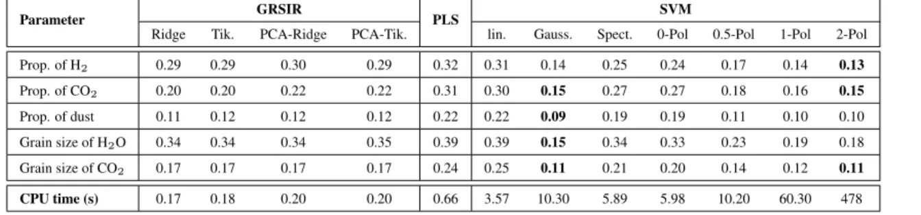
Table 2. NRMSE and computing time for GRSIR, PLS and SVM with various kernels. “x-Pol” is q= x in the polynomial kernel. The power of the polynomial kernel was fixed to 9 for each parameter, after cross-validation. The bottom line of the table corresponds to the training time of parameter “Prop. of H2O” after the selection of optimal hyperparameters.
Parameter GRSIR PLS SVM
Ridge Tik. PCA-Ridge PCA-Tik. lin. Gauss. Spect. 0-Pol 0.5-Pol 1-Pol 2-Pol
Prop. of H2 0.29 0.29 0.30 0.29 0.32 0.31 0.14 0.25 0.24 0.17 0.14 0.13 Prop. of CO2 0.20 0.20 0.22 0.22 0.31 0.30 0.15 0.27 0.27 0.18 0.16 0.15 Prop. of dust 0.11 0.12 0.12 0.12 0.22 0.22 0.09 0.19 0.19 0.11 0.10 0.10 Grain size of H2O 0.34 0.34 0.34 0.35 0.39 0.39 0.15 0.34 0.33 0.23 0.19 0.18 Grain size of CO2 0.17 0.17 0.17 0.17 0.24 0.25 0.11 0.21 0.20 0.14 0.12 0.11 CPU time (s) 0.17 0.18 0.20 0.20 0.66 3.57 10.30 5.89 5.98 10.20 60.30 478
with m ∈ {1, . . . , d}. Table 1 sums up the different strategies we have proposed. ϕ controls which directions ofΣ that are favored: For instance, with the classical SIR approach (first row of Table 1) direction corresponding to small variances are most likely, while no directions are privileged with ridge regularization. For Tikhonov regularization, directions corresponding to large variance are most likely, in contrast to classical SIR. PCA based regularization ap-proaches correspond to the situation where only directions with large variance are kept, i.e., a dimension reduction ofΣ is done. Once β is computed, a piecewise linear estimator is used, i.e. f in eq. (2) is a 1-dimensional piecewise linear function.
3. DATA SETS
In this paper, real and simulated data sets are used. Real data have been collected during orbit 41 61 and 103 by the imaging spectrom-eter OMEGA on board Mars Express Mission. A detailed analysis of this image by an expert led to a surface reflectance model [1]. This model allows by radiative transfer calculations the generation of many synthetic spectra with the corresponding physical parameters: The proportions of CO2, water and dust; and the grain sizes of water and CO2. Centered multiGaussian noise has been added, its covari-ance matrix was determined experimentally from the real image. For the validation sake, separate training and testing datasets have been generated. The notations are the following: n (respectively nt) is the number of spectra from the training data (respectively test data), xi ∈ Rd, i ∈ 1, . . . , n denotes the spectra from the training data and ypi ∈ R, i ∈ 1, . . . , n, p ∈ 1, . . . , 5, is one of the 5 associated parameters (respectivelyxˇj, ˇyp
j, j ∈ 1, . . . , nt). In these experi-ments, n= 3584, nt = 3528 and the number of spectral bands is d= 184. Each parameter takes a finite number of values regularly distributed in a given interval of variation. The different realizations of the vector ypi are generated by building all possible combinations of the individual parameter values. In the following, the index p is omitted in y and in its associated functional f : fp(x) = yp
is written f(x) = y.
For validation purpose, see Section 4, spectra from several im-ages of the same area of Mars where extracted. They correspond to three acquisitions at different times. All the spectra were atmospher-ically corrected.
4. EXPERIMENTS
In all experiments, parameters were selected by a 5-fold cross vali-dation. The quality of the estimation is assessed by computing the Normalized Root Mean Square Errors (NRMSE):
NRMSE= v u u u u u t 1 nt nt P i=1 (ˆyi− ˇyi)2 1 nt nt P i=1 (ˇyi− y)2 with y= 1 nt nt X i=1 ˇ yi (6)
whereyiˇ is the real value andyiˆ the estimated one. NRMSEis close to zero when the predicted values are accurate and becomes larger when predictions are poor. Results are reported in Table 2.
From the table, the worst results in terms of NRMSE are ob-tained with linear algorithms: PLS and SVM with the linear ker-nel. Non-linear SVM provides the best results in terms of accuracy, for both Gaussian and inhomogeneous polynomial kernels. Spec-tral or homogeneous polynomial kernel provide the lowest accuracy for non-linear SVM. For the GRSIR approaches, results are nearly the same, and less accurate than non-linear SVM. The different reg-ularization methods yield the same results, however regreg-ularization parameters (τ and m) are set to different values: Using PCA based regularization, τ is in general set to a lower value than with non-PCA based regularization. Furthermore, β is not the same depending on the regularization. For instance,cos`βridge, βpca-ridge
´
= 0.87 and cos`βridge, βTik.´ = 0.93.
Considering the training time, SVM based approaches lead to the longer processing times, for every kernel and GRSIR is the fastest. Because of the diagonalization of the covariance matrix in eq. (5), PCA based regularization is a little longer. Note that the SVM solver was the LIBSVM, which is a higly optimized C++ solver, while the GRSIR was naively implemented in Matlab. Thus the difference may be higher after a proper implementation of GRSIR.
Inversions are performed on the real data using the functional f . We have considered only the best SVM (Gaussian kernel) and the best GRSIR (ridge). Since no ground data is available, the inversion accuracy is difficult to appreciate quantitatively. We used two sub-jective criteria: the physical possibility, e.g., proportion is greater than 0 and lower than 1, and the stability of estimations over the time, e.g., estimations from the same area at closed dates should be closed.
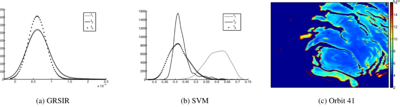
Fig. 1.(a) and Fig. 1.(b) present the estimation of the
“propor-tion of dust”. It can be seen that estimations are very different from GRSIR and SVM. Estimates provided by GRSIR are more realis-tic: First, the range is around10−3which is physically acceptable; second, the variation of the proportion between two dates is low in agreement with experts analysis. On the opposite, SVM estimations are not convincing since the range of the estimations is not realis-tic. This phenomenon can be mitigated by a suitable selection of the simulated training set, as detailed in [12, 13]. The idea is to select training samples that are similar to those to be inverted. However,
! !"# $ $"# % %"# &'$!!( ! %!! )!! *!! +!! $!!! $%!! $)!! $*!! $+!! ' ' , $ , % , ( 0.3 0.35 0.4 0.45 0.5 0.55 0.6 0.65 0.7 0.75 0 200 400 600 800 1000 1200 1400 1600 t 1 t2 t 3
(a) GRSIR (b) SVM (c) Orbit 41
Fig. 1. (a) GRSIR and (b) SVM: Histogram of the “proportion of dust” estimates from real data from the same geographical area acquired at different dates (t1, t2and t3). (c) Estimation of the “proportion of dust” of orbit 41.
this step is time consuming and still does not provide satisfactory results with SVM.
Fig. 1.(c) presents the observation 41 by GRISR for the param-eter “proportion of dust”. The mapping is very smooth and the pro-portion of dust increases significantly with proximity to the bound-aries.
5. DISCUSSION
A machine learning discussion is done in this section. We let read-ers interested in a detailed astrophysical analysis consult the refer-ence [6].
Non-linear SVMs provide very accurate results in term of
NRMSE on the simulated data sets. It comes with an increased training time, which can be critical with the polynomial kernel. Therefore, Gaussian kernel should be preferably used. The defini-tion of new kernels handling more efficiently the physical model is under investigation. The GRSIR approach provides less accurate results on the simulated data sets, but it performs better than SVM of real data sets and his training is very fast.
The regularization strategy does not influence too much the re-sults once the optimal parameters have been found, the key point is to regularize. In the experiments, all the parameters have been se-lected by cross-validation using the simulated data sets. In the con-text of our work (training on simulated data and validation on real data), this strategy should be changed. Statistical differences exist between the simulated data and real data, depending on the geome-try of the observed image and the atmospheric effects. For instance, the cosine angle, computed with the Frobenius inner product, be-tween the covariance matrixΣ of simulated data and the real data is 0.60. We are currently working on a semi-supervised framework to match statistics from simulated data and real data before the es-timation of the regression function. This should improve the results obtained on real data sets.
As a conclusion, handling efficiently the inversion of hyperspec-tral images is possible and of an interest for astrophysicists. First re-sults are promising yet some works are still needed to obtain a fully automatised framework.
6. REFERENCES
[1] S. Dout´e, B. Schmitt, R. M. C. Lopes-Gautier, R. W. Carlson, L. Soderblom, and J. Shirley, “Mapping SO2frost on Io by the modeling of NIMS hyperspectral images,” Icarus, vol. 149, pp. 107–132, 2001.
[2] R. W. Carlson, P. R. Weissman, W. D. Smythe, J. C. Mahoney, the NIMS Science, and Engineering Teams, “Near infrared spectrometer experiment on Galileo,” Space Science Reviews, vol. 60, pp. 457–502, 1992.
[3] D.S. Kimes, Y. Knyazikhin, J.L. Privette, A.A. Abuegasim, and F. Gao, “Inversion methods for physically-based models,”
Re-mote Sensing Reviews, vol. 18, pp. 381–439, 2000.
[4] T. Hastie, R. Tibshirani, and J. Friedman, The Elements of
Statistical Learning: Data Mining, Inference, and Prediction, Springer, 2003.
[5] C. Bernard-Michel, L. Gardes, and S. Girard, “Gaussian reg-ularized sliced inverse regression,” Statistics and Computing, vol. 19, pp. 85–98, 2009.
[6] C. Bernard-Michel, S. Dout´e, M. Fauvel, L. Gardes, and S. Gi-rard, “Retrieval of mars surface physical properties from omega hyperspectral images using regularized sliced inverse regression,” Journal of Geophysical Research, To appear, 2009.
[7] M. Fauvel, J. Chanussot, and J. A. Benediktsson, “Evaluation of kernels for multiclass classification of hyperspectral remote sensing data,” in IEEE ICASSP’06, May 2006.
[8] N. Keshava, “Distance metrics and band selection in hyper-spectral processing with application to material identification and spectral librairies,” IEEE Trans. Geosci. Remote Sens., vol. 42, pp. 1552–1565, July 2004.
[9] K.C. Li, “Sliced inverse regression for dimension reduction,”
Journal of the American Statistical Association, vol. 86, pp. 316–327, 1991.
[10] A. Tarantola, Inverse problem theory and model parameter
estimation, SIAM, 2005.
[11] R.C. Aster, B. Borchers, and C.H. Thurber, Parameter
Estima-tion and Inverse Problems, Elsevier Academic Press, 2005. [12] C. Bernard-Michel, S. Dout´e, L. Gardes, and S. Girard,
“In-verting hyperspectral images with gaussian regularized sliced inverse regression,” in European Symposium on Artificial
Neu-ral Networks, Advances in Computational Intelligence and Learning, 2008.
[13] C. Bernard-Michel, S. Dout´e, M. Fauvel, L. Gardes, and S. Gi-rard, “Support vectors machines regression for the estimation of Mars surface physical properties,” in European Symposium
on Artificial Neural Networks, Advances in Computational In-telligence and Learning, 2009.