Distributed Halide
The MIT Faculty has made this article openly available.
Please share
how this access benefits you. Your story matters.
Citation
Denniston, Tyler, Shoaib Kamil, and Saman Amarasinghe.
“Distributed Halide.” Proceedings of the 21st ACM SIGPLAN
Symposium on Principles and Practice of Parallel Programming
-PPoPP ’16 (2016).
As Published
http://dx.doi.org/10.1145/2851141.2851157
Publisher
Association for Computing Machinery
Version
Final published version
Citable link
http://hdl.handle.net/1721.1/110762
Terms of Use
Creative Commons Attribution-NonCommercial-NoDerivs License
Distributed Halide
Tyler Denniston
MIT [email protected]Shoaib Kamil
Adobe [email protected]Saman Amarasinghe
MIT [email protected]Abstract
Many image processing tasks are naturally expressed as a pipeline of small computational kernels known as stencils. Halide is a popu-lar domain-specific language and compiler designed to implement image processing algorithms. Halide uses simple language con-structs to express what to compute and a separate scheduling co-language for expressing when and where to perform the compu-tation. This approach has demonstrated performance comparable to or better than hand-optimized code. Until now, however, Halide has been restricted to parallel shared memory execution, limiting its performance for memory-bandwidth-bound pipelines or large-scale image processing tasks.
We present an extension to Halide to support distributed-memory parallel execution of complex stencil pipelines. These ex-tensions compose with the existing scheduling constructs in Halide, allowing expression of complex computation and communication strategies. Existing Halide applications can be distributed with minimal changes, allowing programmers to explore the tradeoff between recomputation and communication with little effort. Ap-proximately 10 new of lines code are needed even for a 200 line, 99 stage application. On nine image processing benchmarks, our extensions give up to a 1.4× speedup on a single node over regular multithreaded execution with the same number of cores, by miti-gating the effects of non-uniform memory access. The distributed benchmarks achieve up to 18× speedup on a 16 node testing ma-chine and up to 57× speedup on 64 nodes of the NERSC Cori supercomputer.
Categories and Subject Descriptors D.3.2 [Programming
Lan-guages]: Distributed and Parallel Languages
Keywords Distributed memory; Image processing; Stencils
1. Introduction
High-throughput and low-latency image processing algorithms are of increasing importance due to their wide applicability in fields such as computer graphics and vision, scientific and medical vi-sualization, and consumer photography. The resolution and fram-erate of images that must be processed is rapidly increasing with the improvement of camera technology and the falling cost of stor-age space. For example, the Digitized Sky Survey [1] is a collec-tion of several thousand images of the night sky, ranging in res-olution from 14,000×14,000 to 23,040×23,040 pixels, or 200 to
Permission to make digital or hard copies of part or all of this work for personal or classroom use is granted without fee provided that copies are not made or distributed for profit or commercial advantage and that copies bear this notice and the full citation on the first page. Copyrights for third-party components of this work must be honored. For all other uses, contact the Owner/Author.
PPoPP ’16, March 12-16, 2016, Barcelona, Spain ACM 978-1-4503-4092-2/16/03. http://dx.doi.org/10.1145/2851141.2851157
500 megapixels. Canon, a consumer-grade camera manufacturer, recently introduced a 250 megapixel image sensor [2]. Processing such large images is a non-trivial task: on modern multicore hard-ware, a medium-complexity filter such as a bilateral grid [12] can easily take up to 10 seconds for a 500 megapixel image.
Halide [29], a domain-specific language for stencil pipelines, is a popular high-performance image processing language, used in Google+ Photos, and the Android and Glass platforms [28]. A major advantage of Halide is that it separates what is being computed (the algorithm) from how it is computed (the schedule), enabling programmers to write the algorithm once in a high-level language, and then quickly try different strategies to find a high-performing schedule. Halide code often outperforms hand-written expert-optimized implementations of the same algorithm.
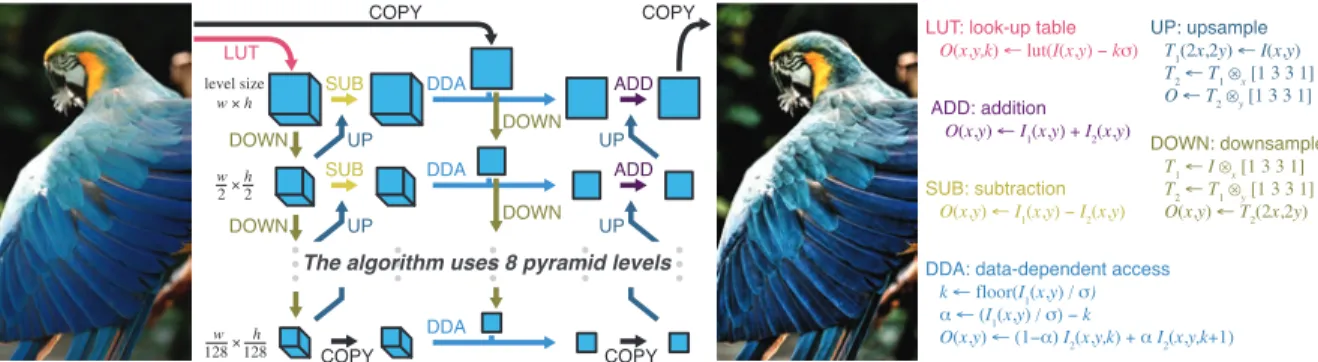
When many stencils are composed into deep pipelines such as the local Laplacian filter [27], the inter-stage data dependen-cies easily become very complex, as visualized in Figure 1. In the case of a local Laplacian filter, many different resampling, data-dependent gathers and horizontal and vertical stencils com-bine to create a complex network of dependencies. Such complex-ity makes rewriting a program to experiment with different opti-mization strategies for computation extremely time consuming. A programmer can easily explore this space with Halide’s separation of algorithm and schedule.
Halide is currently limited to shared-memory execution. For the common case where an image processing pipeline is memory-bandwidth bound, the performance ceiling of these tasks is solely determined by the memory bandwidth of the executing system. Adding additional parallelism with more threads for such pipelines therefore does not result in higher performance. And, with mod-ern multi-socket platforms embracing a non-uniform memory ac-cess (NUMA) architecture, simplistic parallel scheduling such as the work queue used by Halide often achieves poor parallel effi-ciency due to frequent misses into remote memory or cache. When processing today’s images of 100s of megapixels, shared-memory execution limits potential performance.
We address this challenge with our distributed language and compiler extensions. By augmenting Halide programs with the ability to seamlessly distribute data and execution across many compute nodes, we offer the ability to overcome the limitations of shared-memory pipelines with very little effort. Distributed Halide pipelines gain access to more parallelism and increased memory bandwidth, and exhibit better hardware utilization of each individ-ual node. The language extensions for distribution fit well within the existing scheduling language constructs, which can still be used to explore schedules for the on-node computation. The ability to use the a single scheduling language for both distribution and on-node scheduling is important, since depending on the distribution strategy, different on-node schedules yield the best overall perfor-mance.
DOWN DOWN
DOWN
LUT
LUT: look-up table O(x,y,k) lut(I(x,y) k )
DDA: data-dependent access k floor(I1(x,y) ) (I1(x,y) ) k
O(x,y) (1 ) I2(x,y,k) I2(x,y,k 1) DDA
DDA
ADD: addition O(x,y) I1(x,y) I2(x,y)
DOWN DOWN: downsample T1 I x[1 3 3 1] T2 T1 y[1 3 3 1] O(x,y) T2(2x,2y) UP: upsample T1(2x,2y) I(x,y) T2 T1 x[1 3 3 1] O T2 y[1 3 3 1] UP UP SUB SUB: subtraction O(x,y) I1(x,y) I2(x,y)
COPY COPY SUB UP DDA COPY COPY UP ADD ADD
The algorithm uses 8 pyramid levels
level size w h w h 2 2 w h 128 128
Figure 1. Imaging pipelines employ large numbers of interconnected, heterogeneous stages. Here we show the structure of the local Laplacian filter [3, 22], which is used for a variety of tasks in photographic post-production. Each box represents intermediate data, and each arrow represents one or more functions that define that data. The pipeline includes horizontal and vertical stencils, resampling, data-dependent gathers, and simple pointwise functions.
and computer graphics, where stencils are common, but often in a very different form: stencil pipelines. Stencil pipelines are graphs of different stencil computations. Iteration of the same stencil occurs, but it is the exception, not the rule; most stages apply their stencil only once before passing data to the next stage, which performs different data parallel computation over a different stencil.
Graph-structured programs have been studied in the context of streaming languages [4, 11, 29]. Static communication analy-sis allows stream compilers to simultaneously optimize for data parallelism and producer-consumer locality by interleaving compu-tation and communication between kernels. However, most stream compilation research has focussed on 1D streams, where sliding win-dow communication allows 1D stencil patterns. Image processing pipelines can be thought of as programs on 2D and 3D streams and stencils. The model of computation required by image processing is also more general than stencils, alone. While most stages are point or stencil operations over the results of prior stages, some stages gather from arbitrary data-dependent addresses, while others scatter to arbitrary addresses to compute operations like histograms.
Pipelines of simple map operations can be optimized by tradi-tional loop fusion: merging multiple successive operations on each point into a single compound operation improves arithmetic intensity by maximizing producer-consumer locality, keeping intermediate data values in fast local memory (caches or registers) as it flows through the pipeline. But traditional loop fusion does not apply to stencil operations, where neighboring points in a consumer stage depend on overlapping regions of a producer stage. Instead, sten-cils require a complex tradeoff between producer-consumer locality, synchronization, and redundant computation. Because this tradeoff is made by interleaving the order of allocation, execution, and com-munication of each stage, we call it the pipeline’s schedule. These tradeoffs exist in scheduling individual iterated stencil computations in scientific applications, and the complexity of the choice space is reflected by the many different tiling and scheduling strategies introduced in past work [10, 16, 19]. In image processing pipelines, this tradeoff must be made for each producer-consumer relationship between stages in the graph—often dozens or hundreds—and the ideal schedule depends on the global interaction among every stage, often requiring the composition of many different strategies. 1.2 Contributions
Halide is an open-source domain-specific language for the complex image processing pipelines found in modern computational pho-tography and vision applications [26]. In this paper, we present the optimizing compiler for this language. We introduce:
• a systematic model of the tradeoffs between locality, parallelism, and redundant recomputation in stencil pipelines;
• a scheduling representation that spans this space of choices;
• a DSL compiler based on this representation that combines
Halide programs and schedule descriptions to synthesize points anywhere in this space, using a design where the choices for how to execute a program are separated not just from the definition of what to compute, but are pulled all the way outside the black box of the compiler;
• a loop synthesizer for data parallel pipelines based on simple
interval analysis, which is simpler and less expressive than polyhedral model, but more general in the class of expressions it can analyze;
• a code generator that produces high quality vector code for
image processing pipelines, using machinery much simpler than the polyhedral model;
• and an autotuner that can infer high performance schedules—up
to 5⇥ faster than hand-optimized programs written by experts— for complex image processing pipelines using stochastic search. Our scheduling representation composably models a range of tradeoffs between locality, parallelism, and avoiding redundant work. It can naturally express most prior stencil optimizations, as well as hierarchical combinations of them. Unlike prior stencil code generation systems, it does not describe just a single stencil scheduling strategy, but separately treats every producer-consumer edge in a graph of stencil and other image processing computations. Our split representation, which separates schedules from the underlying algorithm, combined with the inside-out design of our compiler, allows our compiler to automatically search for the best schedule. The space of possible schedules is enormous, with hundreds of inter-dependent dimensions. It is too high dimensional for the polyhedral optimization or exhaustive parameter search employed by existing stencil compilers and autotuners. However, we show that it is possible to discover high quality schedules using stochastic search.
Given a schedule, our compiler automatically synthesizes high quality parallel vector code for x86 and ARM CPUs with SSE/AVX and NEON, and graphs of CUDA kernels interwoven with host management code for hybrid GPU execution. It automatically infers all internal allocations and a complete loop nest using simple but general interval analysis [18]. Directly mapping data parallel dimensions to SIMD execution, including careful treatment of strided access patterns, enables high quality vector code generation, without requiring any general-purpose loop auto-vectorization.
Figure 1: Data dependencies in a local Laplacian filter. Each box represents intermediate data, and arrows represent functions (color-coded with their bodies on the right) defining the data. Image reproduced with permission from [29].
1.1 Contributions
In this paper, we present language extensions for distributing pipelines and a new compiler backend that generates distributed code. In particular, the contributions of this paper are:
•A Halide language extension for distributing image processing
pipelines, requiring programmers to write only approximately 10 new lines of code. We show that it is possible to describe complex organizations of data and computation both on-node and across multiple machines using a single, unified scheduling language.
•The implementation of a Halide compiler backend generating
distributed code via calls to an MPI library.
•A demonstration of how distributed pipelines can achieve a
1.4× speedup on a single node with the same number of cores over regular multithreaded execution by mitigating NUMA ef-fects.
•Evaluation of nine distributed image processing benchmarks
scaling up to 2,048 cores, with an exploration of redundant work versus communication tradeoff.
The rest of this paper is organized as follows. Section 2 sum-marizes the necessary background on Halide including simple scheduling semantics. Section 3 introduces the new distributed scheduling directives. Section 4 discusses distributed code gener-ation and Section 5 evaluates distributed Halide on several image processing benchmarks. Section 6 discusses related work, and Sec-tion 7 concludes.
2. Halide Background
Halide [29] is a domain-specific language embedded in C++ for im-age processing. One of its main points of novelty is the fundamen-tal, language-level separation between the algorithm and schedule for a given image processing pipeline. The algorithm specifies what is being computed, and the schedule specifies how the computation takes place. By separating these concerns in the language, a pro-grammer only writes an algorithm once. When hardware require-ments change, or new features such as larger vector registers or larger caches become available, the programmer must only modify the schedule to take advantage of them.
As a concrete example, consider a simple 3×3 box blur. One typical method to compute this is a 9-point stencil, computing an output pixel as the average value of the neighboring input pixels. In Halide, such a blur can be expressed in two stages: first a horizontal blur over a 1×3 region of input pixels, followed by a vertical 3×1
blur. This defines the algorithm of the blur, and is expressed in Halide as:
bh(x, y) = (in(x-1, y) + in(x, y) + in(x+1, y)) / 3; bv(x, y) = (bh(x, y-1) + bh(x, y) + bh(x, y+1)) / 3;
where each output pixel output(x,y) = bv(x,y).
Halide schedules express how a pipeline executes. For example, one natural schedule computes the entire bh horizontal blur stage before computing the bv stage. In Halide’s scheduling language, this is known as computing the function at “root” level, and is expressed as:
bh.compute_root();
With this schedule, our blur pipeline is compiled to the following pseudo-code of memory allocations and loop nests:
allocate bh[] for y:
for x:
bh[y][x] = (in[y][x-1] + in[y][x] + in[y][x+1]) / 3 for y:
for x:
bv[y][x] = (bh[y-1][x] + bh[y][x] + bh[y+1][x]) / 3
By opting to completely compute the horizontal blur before begin-ning the vertical blur, we schedule the pipeline such that there is no redundant computation: each intermediate pixel in bh is only calculated once. However, this sacrifices temporal locality. A pixel stored into the bh temporary buffer may not be available in higher levels of the memory hierarchy by the time it is needed to compute bv. This time difference is known as reuse distance: a low reuse distance is equivalent to good temporal locality.
Because the horizontal blur is so cheap to compute, a better schedule may compute pixels of bh multiple times to improve reuse distance. One possibility is to compute a subset of the horizontal blur for every row of the vertical blur. Because a single row of the vertical blur requires three rows in bh (the row itself and the rows above and below), we can compute only those three rows of bh in each iteration of bv.y. In Halide, the schedule:
bh.compute_at(bv, y);
is lowered to the loop nest:
for y:
allocate bh[]
for y’ from y-1 to y+1: for x:
bh[y’][x]=(in[y’][x-1] + in[y’][x] + in[y’][x+1])/3 for x:
Note that the inner iteration of y’ ranges from y-1 to y+1: the in-ner loop nest is calculating the currently needed three rows of bh. Some details such as buffer indexing and how the Halide compiler determines loop bounds have been elided here for clarity, but the essence is the same. The tradeoff explored by these two schedules is that of recomputation versus locality. In the first schedule, there is no recomputation, but locality suffers, while in the second sched-ule, locality improves, as values in bh are computed soon before they are needed, but we redundantly compute rows of bh.
Halide also offers a simple mechanism for adding parallelism to pipelines on a per-stage per-dimension basis. To compute rows of output pixels in parallel, the schedule becomes:
bh.compute_at(bv, y); bv.parallel(y);
which is lowered to the same loop nest with the outermost bv.y loop now a parallel for loop. The runtime mechanism for support-ing parallel for loops encapsulates iterations of the parallel dimen-sion bv.y into function calls with a parameter specifying the value of bv.y to be computed. Then, a work queue of all iterations of
bv.yis created. A runtime thread pool (implemented using e.g.
pthreads) pulls iterations from the work queue, executing iterations in parallel. This dynamic scheduling of parallelism can be a source of cache inefficiencies or NUMA effects, as we explore in Sec-tion 5.
Designing good schedules in general is a non-trivial task. For blur the most efficient schedule we have found, and the one we compare against in our evaluation is:
bh.store_at(bv, y).compute_at(bv, yi).vectorize(x, 8); bv.split(y, y, yi, 8).vectorize(x, 8).parallel(y);
For large pipelines such as the local Laplacian benchmark consist-ing of approximately 100 stages, the space of possible schedules is enormous. One solution to this problem is applying an autotuning system to automatically search for efficient schedules, as was ex-plored in [29]. Other more recent autotuning systems such as Open-Tuner [9] could also be applied to the same end.
3. Distributed Scheduling
One of the major benefits of the algorithm-plus-schedule approach taken by Halide is the ability to quickly experiment to find an ef-ficient schedule for a particular pipeline. In keeping with this phi-losophy, we designed our distributed Halide language extensions to be powerful enough to express complex computation and commu-nication schemes, but simple enough to require very little effort to find a high-performance distributed schedule.
There are many possible language-level approaches to express data and computation distributions. We strove to ensure that the new scheduling constructs would compose well with the exist-ing language both in technical (i.e. the existexist-ing compiler should not need extensive modification) and usability terms. The new ex-tensions needed to be simple enough for programmers to easily grasp but powerful enough to express major tradeoffs present in distributed-memory programs.
Striking a balance between these two points was accomplished by adding two new scheduling directives, distribute() and compute rank(), as well as a new DistributedImage buffer type that uses a simple syntax to specify data distributions. We show that these extensions are simple to understand, compose with the existing language, and allow complex pipelines to be scheduled for excellent scalability.
3.1 Data Distribution via DistributedImage
Input and output buffers in Halide are represented using the user-facing Image type. Images are multidimensional Cartesian grids
of pixels and support simple methods to access and modify pixel values at given coordinates. In distributed Halide, we implemented a user-facing DistributedImage buffer type which supports ad-ditional methods to specify the distribution of data to reside in the buffer.
A DistributedImage is declared by the user with the di-mensions’ global extents and names. A data distribution for each
DistributedImageis specified by the user by using the
placement()method, which returns an object supporting a
sub-set of the scheduling directives used for scheduling Halide func-tions, including the new distribute() directive. “Scheduling” the placement specifies a data distribution for that image. The fol-lowing example declares a DistributedImage with global ex-tents width and height but distributed along the y dimension.
DistributedImage<int> input(width, height); input.set_domain(x, y);
input.placement().distribute(y); input.allocate();
It is important to note that the amount of backing memory allocated on each rank with the allocate() call is only the amount of the per-rank size of the image. The size of the local region is determined by the logic explained next in Section 3.2. The call to allocate() must occur separately and after all scheduling has been done via placement() in order to calculate the per-rank size. For a rank to initialize its input image, the DistributedImage type supports conversion of local buffer coordinates to global coor-dinates and vice versa. This design supports flexible physical data distributions. For example, if a monolithic input image is globally available on a distributed file system, each rank can read only its local portion from the distributed file system by using the global coordinates of the local region. Or, if input data is generated al-gorithmically, each rank can initialize its data independently using local or global coordinates as needed. In either case, at no point does an individual rank allocate or initialize the entire global image. Output data distribution is specified in exactly the same manner. 3.2 Computation Distribution
To support scheduling of distributed computations, we introduce two new scheduling directives: distribute() and compute rank().
The distribute() directive is applied to dimensions of indi-vidual pipeline stages, meaning each stage may be distributed in-dependently of other stages. Because dimensions in Halide corre-spond directly to levels in a loop nest, a distributed dimension cor-responds to a distributed loop in the final loop nest. The iteration space of a distributed loop dimension is split into slices accord-ing to a block distribution. Each rank is responsible for exactly one contiguous slice of iterations of the original loop dimension.
The compute rank() directive is applied to an entire pipeline stage, specifying that the computed region of the stage is the region required by all of its consumers on the local rank (we adopt the MPI terminology “rank” to mean the ID of a distributed process). Scheduling a pipeline stage with compute rank() ensures that lo-cally there will be no redundant computation, similar to the se-mantics of compute root() in existing Halide. However, different ranks may redundantly compute some regions of compute rank functions. Therefore, compute rank() allows the expression of globally redundant but locally nonredundant computation, a new point in the Halide scheduling tradeoff space.
The block distribution is defined as follows. Let R be the num-ber of MPI processes or ranks available and let w be the global extent of a loop dimension being distributed. Then the slice size
s=dw/Re, and each rank r is responsible for iterations
Rank 0 Rank 1 Rank 2 input
f.x
0 3 4 7 8 9
Figure 2: Communication for 1D blur. Dotted lines represent on-node access, solid lines represent communication.
where [u, v) denotes the half-open interval from u to v. This has the effect of assigning the last rank fewer iterations in the event R does not evenly divide w.
The slicing of the iteration space is parameterized by the total number of ranks R and the current rank r. Our code generation (explained in Section 4) uses symbolic values for these parameters; thus, running a distributed Halide pipeline on different numbers of ranks does not require recompiling the pipeline.
The distribute() directive can also be applied to two or three dimensions of a function to specify multidimensional (or nested) distribution. For nested distribution, the user must specify the size of the desired processor grid to distribute over: we currently do not support parametric nested distributions as in the one dimensional case. The nested block distribution is defined as follows. Let x and
yrespectively be the inner and outer dimensions in a 2D nested
distribution, let w and h be their respective global extents and let a and b be the respective extents of the specified processor grid. Then
the slice sizes are sx =dw/ae and sy = dh/be. Each rank r is
responsible for a 2D section of the original iteration space, namely:
x∈ [r (mod a)sx, min(w, (r (mod a) + 1)sx))
y∈ [(r\a)sy, min(h, (r\a + 1)sy))
where u\v denotes integer division of u and v. For 3D distribution, letting d be the extent of the third dimension z, c be the third extent
of the specified processor grid, sz =dd/ce, the iteration space for
rank r is:
x∈ [(r (mod ab)) (mod a)sx,
min(w, ((r (mod ab)) (mod a) + 1)sx))
y∈ [((r (mod ab))\a)sy,
min(h, (((r (mod ab))\a) + 1)sy))
z∈ [(r\(ab))sz, min(d, (r\(ab) + 1)sz)).
3.3 Introductory Example
As an example, consider a simple one-dimensional blur operation:
f(x) = (input(x - 1) + input(x + 1)) / 2;
We can distribute this single-stage pipeline using the two new language features (eliding the boilerplate set domain() and
allocate()calls):
DistributedImage input(width); input.placement().distribute(x); f.distribute(x);
With this schedule, the input buffer is distributed along the same dimension as its consumer stage f.
We call the slice of the input buffer residing on each rank the owned region. Because f is a stencil, we must also take into account the fact that to compute an output pixel f(x) requires input(x-1) and input(x+1). We denote this the required region of buffer input.
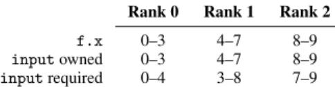
Suppose that the width of input is 10 pixels, and we have 3 ranks to distribute across. Then the following table enumerates each rank’s owned and required regions of input, according to the distributed schedule:
Rank 0 Rank 1 Rank 2
f.x 0–3 4–7 8–9
inputowned 0–3 4–7 8–9
inputrequired 0–4 3–8 7–9
Because the input buffer is distributed independently from its consumer, and distributed slices are always disjoint by construc-tion, the required region is larger than the owned region for buffer input. Therefore, the required values of input will be communi-cated from the rank that owns them. In this example, rank 1 will send input(4) to rank 0 and input(7) to rank 2 (and receive from both ranks 0 and 2 as well). The communication is illustrated in Figure 2.
The region required but not owned is usually termed the ghost zone (see e.g. [22]), and the process of exchanging data is called border exchange or boundary exchange. In distributed Halide, ghost zones are automatically inferred by the compiler based on the schedule, and the communication code is inserted automati-cally. The mechanics of how the ghost zones are calculated and communicated are detailed in Section 4.
This example describes a single-stage pipeline, but for multi-stage pipelines, data must be communicated between the multi-stages. Between each distributed producer and consumer, ghost zones are determined and communication code is automatically inserted by the compiler, just as the case above of communicating input to the ranks computing f.
3.4 Recomputation versus Communication
A fundamental tradeoff exposed by the new distribute() and
compute rank() scheduling directives is recomputation versus
communication. In some cases, it may be advantageous to locally recompute data in the ghost zone, instead of communicating it ex-plicitly from the rank that owns the data. While there are models of distributed computation and communication (e.g. [7]) that can be applied to make one choice over the other, these models are neces-sarily approximations of the real world. For optimal performance, this choice should be made empirically on a per-application basis. With distributed Halide, we can explore the tradeoff not just per application, but per stage in an image processing pipeline.
In distributed Halide, there are three points on the spectrum of this tradeoff. Globally and locally non-redundant work is expressed by the compute root()+distribute() directives, ensuring the function is computed exactly once by a single rank for a given point in the function’s domain. This is the typical case, but communica-tion may be required for consumers of a pipeline stage distributed in this manner. Globally redundant but locally non-redundant work is expressed by the new compute rank() directive, meaning a given point in the function domain may be computed by multiple ranks, but on each rank it is only ever computed once. No com-munication is required in this case, as each rank computes all of the data it will need for the function’s consumers. Finally, globally and locally redundant work is expressed by scheduling a function
compute atinside of its distributed consumer. A given point in the
function domain may be computed multiple times within a single rank as well as across ranks, but no communication is required.
No one point on this tradeoff spectrum is most efficient for all applications. Distributed Halide exposes this tradeoff to the user, allowing the best choice to be made on a case-by-case basis.
Recalling the 3×3 box blur example from Section 2, this dis-tributed schedule expresses globally and locally redundant compu-tation of bh:
bh.compute_at(bv, y);
bv.parallel(y).distribute(y);
Crucially, even though the pipeline is distributed, there is no com-munication of bh, but instead each rank computes the region of bh
Gn-3 ... Gn Gn-3 ... Gn Input Image G0 G1 G2 Communication Copy Distribution Threshold Rank 0 Rank 1 Rank 2 Gn-3 ... Gn
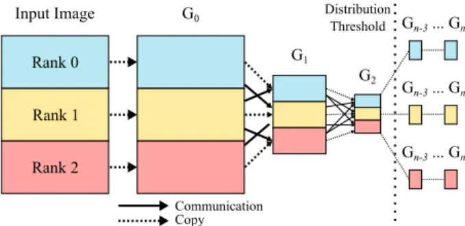
Figure 3: Communication for the Gaussian pyramid computation in the Local Laplacian benchmark. The final three levels after the “distribution threshold” are redundantly computed by every rank. it needs for each of the rows it produces in bv. Because the com-putation of bh occurs within the distributed dimension bv.y, each rank computes bh separately. This means the overlapping rows of
bhthat are required for each iteration of bv.y are computed
redun-dantly and locally. Communication is still required for the region of the input buffer needed to compute the local portion of bv, but no communication is required for the bh stage.
An alternative schedule that contains no redundant computation, but requires communication of both the input buffer and the bh stage is:
bh.compute_root().distribute(y); bv.parallel(y).distribute(y);
The horizontal blur is computed entirely before the vertical blur begins. Before computing bh, the ghost zone data (required but not owned data) of the input buffer must be communicated between ranks. Then, the overlapping rows of bh.y in the ghost zone must be communicated before computation of bv can begin. This is a case where there is no redundant computation (all pixels of bh are computed exactly once globally).
A more extreme version of redundant computation is the fol-lowing:
bh.compute_root();
bv.parallel(y).distribute(y);
With this schedule, the entire horizontal blur (i.e. over the entire global input image) is evaluated on every rank. This is wasteful in terms of computation, as each rank will compute more of bh than it needs. However, locally there is no redundant computation, and globally there is no communication required for bh. Using this particular strategy is crucial for scalability on the local Laplacian benchmark, as shown in Figure 3. The final three stages of the im-age pyramid in Figure 3 are recomputed on every node, as the data is small enough that recomputation is faster than communication.
Finally, this schedule express globally redundant but locally non-redundant computation:
bh.compute_rank();
bv.parallel(y).distribute(y);
Each rank will non-redundantly (i.e. at root level on each rank) compute only the region of bh required to compute the local por-tion of bv. No communicapor-tion is required in this case. However, neighboring ranks will compute overlapping rows of bh, meaning globally there is some redundant computation.
3.5 On-Node Scheduling
The distribute() and compute rank() directives compose with existing Halide scheduling directives. All ranks inherit the same schedule for computing the local portion of a global
compu-tation. To express the common idiom of distributing data across ranks and locally parallelizing the computation on each rank, the parallel() directive can be used in conjunction with the
distribute() directive.The various existing scheduling
direc-tives can be composed arbitrarily to arrive at complex schedules of computation and communication. For example, the following schedule (taken from the block transpose benchmark) causes f to be computed by locally splitting the image into 16 × 16 tiles, vec-torizing and unrolling the computation of each tile, distributing the rows of f and locally parallelizing over the rows of tiles:
f.tile(x, y, xi, yi, 16, 16) .vectorize(xi).unroll(yi) .parallel(y).distribute(y);
The flexibility of this approach allows programmers to specify efficient on-node schedules and freely distribute the computation of each stage, without worrying about calculating ghost zones or writing communication code.
3.6 Limitations
The current implementation of distributed Halide supports all of the features described above, but there are several engineering challenges remaining to be addressed. In particular, ahead of time compilation has not yet been implemented; currently only JITted pipelines can be distributed. Only dimensions that can be paral-lelized can be distributed, i.e. distributing data-dependent dimen-sions (as used in a histogram, for example) is unimplemented. Nested distributions with a parametric processor grid are not yet supported, as previously mentioned in Section 3.2. Any stage writing to a distributed output buffer must currently have the same distribution as the output buffer. Reordering storage with the reorder storage() scheduling directive is not yet supported for distributed dimensions.
4. Code Generation
This section details the new analysis and lowering pass added to the Halide compiler to generate code for distributed pipelines. There are two components of code generation: determining ghost zones for each distributed producer-consumer relationship in the pipeline, and inserting MPI calls to communicate required data in the ghost zones. The mechanisms presented here are similar to those in previous work such as [15] for affine loop nests; see Section 6 for a discussion of their work. The main advantage of our approach lies in the simplicity of ghost zone inference and code generation.
4.1 Ghost Zone Inference
Our ghost zone inference relies heavily on the axis-aligned bound-ing box bounds inference already present in the Halide compiler. In regular Halide, bounds information is needed to determine allo-cation sizes of intermediate temporary memory, iteration spaces of pipeline stages and out-of-bounds checks, among other things.
For each consumer stage in the pipeline, we generate the owned and required information for its inputs, which may be DistributedImages or earlier stages in the pipeline. We derive the owned and required regions in terms of the global buffer bounds the programmer provides via the DistributedImage type.
Recall the iteration space slicing from Section 3.2 and the one-dimensional blur f from Section 3.3. Applying bounds inference to the distributed loop nest generates the symbolic owned and required regions for computing f (omitting boundary conditions for simplicity):
Rank r
f.x rsto (r + 1)s
inputowned rsto (r + 1)s
inputrequired rs− 1 to (r + 1)s + 1
Identical inference is done for every producer-consumer relation-ship in the distributed pipeline. Multidimensional buffers are han-dled with the same code: the bounds inference information gener-alizes across arbitrary dimensions.
Because these regions are parameterized by a rank variable, any particular rank r can determine the owned and required regions for
another rank r0. A global mapping of rank to owned region is never
explicitly computed or stored; instead it is computed dynamically when needed. By computing data locations lazily, we avoid creating and accessing a mapping of global problem space to compute rank. Border exchange is required for the distributed inputs of each consumer in the pipeline. The inputs could be Distributed-Images or earlier distributed stages in the pipeline. In the following discussion we will refer to these collectively as “data sources,” as the owned and required regions are computed the same way no matter the type of input.
To perform a border exchange for data source b between two
ranks r and r0, each must send data it owns to the other rank if it
requires it. Let H(b; r) be the owned (or “have”) region of data source b by rank r and let N(b; r) be the required (or “need”)
region. If H(b; r) intersects N(b; r0), rank r owns data required by
r0, and symmetric send/receive calls must be made on each rank.
The H and N regions are represented by multidimensional axis-aligned bounding boxes, where each dimension has a minimum and maximum value. Computing the intersection I of the two bounding boxes is done using the following equations:
Id(b, r, r0).min = max{Hd(b; r).min, Nd(b; r0).min}
Id(b, r, r0).max = min{Hd(b; r).max, Nd(b; r0).max}
where Bd(·).min/max denotes the minimum or maximum in
di-mension d of bounding box B. We generate the communication code using this static representation of the intersection between
what a rank r has and what a rank r0needs.
The intersections are calculated using global coordinates (rel-ative to the global input/output buffer extents). The actual buffers allocated on each rank are only the size of the local region. Thus, before passing the intersection regions to the MPI library, they must be converted to local coordinates, offset from 0 instead of rs. For rank r and a region X of data source b in global coordinates, we define L(X, b; r) to be X in coordinates local to rank r. L is com-puted by subtracting the global minimum from the global offset to compute a local offset:
Ld(X, b; r).min = Xd.min− Hd(b; r).min
Ld(X, b; r).max = Xd.max− Hd(b; r).min.
4.2 Communication Code Generation
Preceding each consumer stage in the pipeline, we inject MPI calls to communicate the ghost zone region of all distributed inputs required by the stage. This process is called the border exchange.
Generating the code to perform border exchange uses the in-ferred symbolic ghost zone information. For a data source b, the function border exchange(b) is generated with the following body:
function border_exchange(b): let R = mpi_num_ranks() let r = mpi_rank() for r’ from 0 to R-1:
// What r has and r’ needs: let I = intersect(H(b,r), N(b,r’)) // What r needs and r’ has: let J = intersect(H(b,r’), N(b,r)) if J is not empty: let LJ = local(J, b, r) mpi_irecv(region LJ of b from r’) if I is not empty: let LI = local(I, b, r) mpi_isend(region LI of b to r’) mpi_waitall()
The number of ranks R and the current rank r are symbolic values determined at runtime by calls to MPI. Keeping these values sym-bolic means that the bounds inference applied to this loop nest will be in terms of these symbols. This allows us to not require recom-pilation when changing the number of ranks.
A call to the border exchange is inserted preceding the compu-tation of a stage. Recall the distributed one-dimensional blur from Section 3.3. As was illustrated, the owned region of buffer input is smaller than the required region, necessitating border exchange on the input buffer:
let R = mpi_num_ranks() let r = mpi_rank() let s = ceil(w/R) border_exchange(input)
for x from r*s to min(w-1, (r+1)*s): f[x] = (input[x-1] + input[x+1]) / 2
Performing border exchanges for multidimensional buffers re-quires more specialized handling. In particular, the regions of mul-tidimensional buffers being communicated may not be contigu-ous in memory. We handle this case using MPI derived datatypes, which allow a non-contiguous region of memory to be sent or re-ceived with a single MPI call. The MPI implementation automat-ically performs the packing and unpacking of the non-contiguous region, as well as allocation of scratch memory as needed. This, along with wide support on a variety of popular distributed archi-tectures, was among the reasons we chose to use MPI as the target of our code generation.
5. Evaluation
We evaluate distributed Halide by taking nine existing image pro-cessing benchmarks written in Halide and distributing them using the new scheduling directives and the DistributedImage type. The benchmarks range in complexity from the simple two-stage box blur to an implementation of a local Laplacian filter with 99 stages. For each, we begin with the single-node schedule tuned by the author of the benchmark. All schedules are parallelized, and usually use some combination of vectorization, loop unrolling, tiling and various other optimizations to achieve excellent single-node performance. We then modify the schedules to use the dis-tributed Halide extensions. Many of the benchmarks are the same as in the original Halide work [29]. A brief description of each benchmark follows.
Bilateral grid This filter blurs the input image while preserving
edges [12]. It consists of a sequence of three-dimensional blurs over each dimension of the input image, a histogram calculation and a linear interpolation over the blurred results.
Blur An implementation of the simple 2D 9-point box blur filter.
Camera pipe An implementation of a pipeline used in digital
2022242628210212214216218220222
Message size (bytes) 0 100 200300 400500 600700 Latency (us)
(a) Point-to-point latency
2022242628210212214216218220222
Message size (bytes) 01 2 3 45 67 Bandwidth (GB/s) (b) Point-to-point bandwidth
Figure 4: Network point-to-point latency and bandwidth measure-ments for our testing environment.
sensors into a usable digital image. This pipeline contains more than 20 interleaved stages of interpolation, de-mosaicing, and color correction, and transforms a two-dimensional input into a three-dimensional output image.
Interpolate A multi-scale image pyramid [6] is used to
interpo-late an input image at many different resolutions. The image pyra-mid consists of 10 levels of inter-dependent upsampling and down-sampling and interpolation between the two.
Local Laplacian This filter [27] performs a complex
edge-preserving contrast and tone adjustment using an image pyramid approach. The pipeline contains 99 stages and consists of multiple 10-level image pyramids including a Gaussian pyramid and Lapla-cian pyramid. Between each stage are complex and data-dependent interactions, leading to an incredibly large schedule space. This is our most complex benchmark.
Resize This filter implements a 130% resize of the input image
using cubic interpolation, consisting of two separable stages.
Sobel An implementation of image edge-detection using the
well-known Sobel kernel.
Transpose An implementation of a blocked image transpose
al-gorithm.
Wavelet A Daubechies wavelet computation.
Our testing environment is a 16 node Intel Xeon E5-2695 v2 @ 2.40GHz Infiniband cluster with Ubuntu Linux 14.04 and kernel version 3.13.0-53. Each node has two sockets, and each socket has 12 cores, for a total of 384 cores. Hyperthreading is enabled, and the Halide parallel runtime is configured to use as many worker threads as logical cores. The network topology is fully connected.
To analyze the network performance of our test machine we ran the Ohio State microbenchmark suite [26]. The point-to-point MPI latency and effective bandwidth measurements are reported in Figures 4a and 4b respectively.
Due to the presence of hyperthreading and the dynamic load bal-ancing performed by the Halide parallel runtime, the performance numbers had non-negligible noise. As the input size decreases for a multithreaded Halide pipeline, the variance in runtime increases. For a 1000×1000 parallel blur with unmodified Halide, over 1,000 iterations we recorded a standard deviation of 21.3% of the arith-metic mean runtime. At 23,000×23,000, we recorded a standard deviation of 2.1%. In a distributed pipeline, even though the global input may be large enough to lower the variance, each rank has a smaller region of input and therefore higher variance. To miti-gate this variance as much as possible in our measurements of dis-tributed Halide, we take median values of 50 iterations across for each node and report the maximum recorded median. The timing results were taken using
Input Size Distr. Halide OpenCV Speedup
(s) (s) 1000× 1000 0.002 0.002 1.0× 2000× 2000 0.002 0.009 1.255× 4000× 4000 0.004 0.033 8.252× 10000× 10000 0.023 0.223 9.697× 20000× 20000 0.096 0.917 9.552× 50000× 50000 0.688 5.895 8.568×
Table 1: Speedup of Distributed Halide box blur over OpenCV.
Input Size Distr. Halide OpenCV Speedup
(s) (s) 1000× 1000 0.003 0.004 1.020× 2000× 2000 0.004 0.019 4.752× 4000× 4000 0.010 0.074 7.4× 10000× 10000 0.054 0.446 8.259× 20000× 20000 0.183 1.814 9.913× 50000× 50000 1.152 12.674 11.001×
Table 2: Speedup of Distributed Halide Sobel edge detection over OpenCV.
clock gettime(CLOCK MONOTONIC), a timer available on Linux with nanosecond resolution.
We first compare two benchmarks to popular open-source opti-mized versions to illustrate the utility of parallelizing these bench-marks, even at small input sizes. We then report performance of distributed Halide in two categories: scaling and on-node speedup. 5.1 OpenCV Comparison
To establish the utility of using Halide to parallelize and distribute these benchmarks, we first compare against reference sequential implementations of the box blur and edge-detection benchmarks. We chose to compare against OpenCV [4], a widely-used open source collection of many classical and contemporary computer vi-sion and image processing algorithms. The OpenCV implementa-tions have been hand-optimized by experts over the almost 20 years it has been in development.
We chose box blur and edge-detection to compare because OpenCV contains optimized serial implementations of both ker-nels, whereas both Halide benchmarks are fully parallelized. We built OpenCV on our test machine using the highest vectorization settings (AVX) defined by its build system. The results are summa-rized in Tables 1 and 2. For the largest tested input size, the parallel single-node Halide implementation was 8.5× faster for box blur and 11× faster for Sobel. Even for these simple pipelines there is a need for parallelism.
5.2 Scaling
To test the scalability of distributed Halide, we ran each bench-mark on increasing numbers of ranks with a fixed input size. We repeated the scaling experiments with several input sizes up to a maximum value. These results measure the benefit of distributed computation when the communication overhead is outstripped by the performance gained from increased parallelism. As a baseline, for each benchmark and input size, we ran the non-distributed ver-sion on a single node. As mentioned previously, the parallel runtime was configured to use as many threads as logical cores. Therefore, for all benchmarks we normalized to the non-distributed, single-node, 24-core/48-thread median runtime on the given input size.
When increasing the number of nodes, we adopted a strategy of allocating two ranks per node. This maximized our distributed
per-input.distribute(x) output.distribute(y) input.distribute(y)
output.distribute(y)
Figure 6: Two data distributions in transpose. By distributing the in-put along the opposite dimension as the outin-put, only local accesses (dotted lines) are required to transpose the input, as opposed to the explicit communication (solid lines) in the other case.
# nodes Input Distr. Runtime (s) Speedup
1 N/A 0.119 1.0 ×
16 y 0.067 1.779 ×
16 x 0.007 16.172 ×
Table 3: Speedup of transpose on 23000×23000 image with differ-ent input distributions.
formance by mitigating effects of the NUMA architecture, explored in more detail in the following section.
The scaling results from all nine benchmarks are presented in Figure 5. Broadly speaking, the results fall into three categories.
In the first category are the bilateral grid, blur, resize, So-bel, transpose and wavelet benchmarks. This category represents benchmarks exhibiting predictable and well-scaling results. The distribution strategy in bilateral grid, blur and wavelet was the same, utilizing multiple stages with redundant computation. The only data source requiring communication for these benchmarks was the input buffer itself: once the (relatively small) input ghost zones were received, each rank could proceed independently, maxi-mizing parallel efficiency. On bilateral grid, even the smallest input size achieved a 8.8× speedup on 16 nodes, with the maximum in-put size achieving 12.1× speedup. On blur and wavelet, the small-est input size achieved a speedup only around 4×: both blur and wavelet have very low arithmetic complexity, meaning with small input sizes each rank was doing very little computation.
Transpose, which belongs to the first category, demonstrated good scaling when distributing the input and output buffers along opposite dimensions. We distributed the input along the x dimen-sion and output along the y dimendimen-sion, requiring only on-node data access to perform the transpose. If we distributed both the input and output along the same dimension, the ghost zone for the input on each rank would have required communication. These two strate-gies are visualized in Figure 6. In Table 3 we compare the speedup of transpose with 16 nodes using each data distribution. The differ-ence between the two data distributions is an order of magnitude of speedup gained.
The second category consists of camera pipe and local Lapla-cian. These benchmarks exhibit less scalability than those in the first category. Both the camera pipe and local Laplacian pipelines are complex, leading to a large schedule space, and we expect that by exploring further schedules, even better scalability can be achieved. Regardless of their suboptimal schedules, local Laplacian and camera pipe achieved a 7.7× and 11.2× speedup on 16 nodes, respectively, for their largest input sizes.
The final category consists of interpolate. This benchmark displayed superlinear scaling for larger input sizes. The
image-Benchmark 1k/1N 1k/16N 20k/1N 20k/16N
App. MPI% App. MPI% App. MPI% App. MPI%
bilateral grid 2.43 0.04 9.83 53.65 809 0.08 847 2.47 blur 0.19 14.16 5.87 93.46 16.4 0.82 28.8 12.93 camera pipe 0.86 13.24 – – 78.5 0.42 140 28.24 interpolate 1.27 22.64 23.6 68.31 188 3.64 250 44.05 local lapla-cian 3.07 10.5 30.6 61.83 360 6.42 813 72.26 resize 0.6 7.61 3.96 71.45 59.3 1.42 131 42.09 sobel 0.13 12.32 7.16 92.93 18.6 1.22 30.7 23.41 transpose 0.09 7.58 1.01 69.66 9.83 0.10 14.7 39.84 wavelet 0.20 10.81 2.05 66.15 13 0.67 20.9 27.52
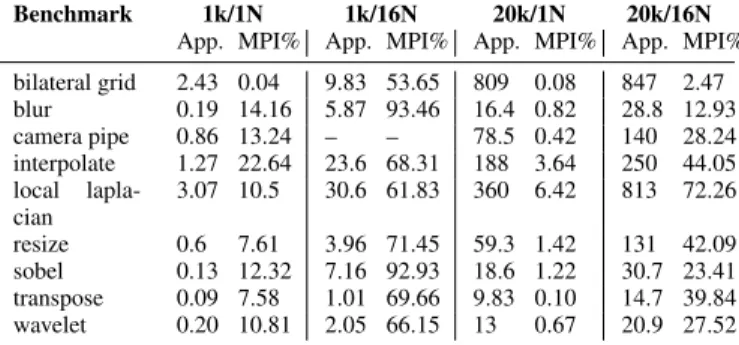
Table 4: Communication and computation time for each bench-mark.
pyramid based interpolation displayed some of the best scaling behavior, even at a maximum input size of 20,000×20,000. We accomplished this in part by utilizing redundant computation in the later stages of the pyramid, using the strategy visualized in Fig-ure 3. In addition, the distributed pipeline exhibits better hardware utilization: as the working set size decreases per rank, each pro-cessor can make more effective use of its cache, leading to better memory bandwidth utilization. Finally, NUMA-aware data parti-tioning leads to better on-node parallel efficiency, and is explored in more detail in the following subsection.
To measure an estimation of scaling efficiency, we also mea-sured the communication overhead for each benchmark on the smallest input and a mid-range input size (1000 × 1000 and
20000× 20000 respectively), on a single node (with two MPI
ranks) and 16 nodes (with 32 MPI ranks, one per socket). We used the MPIP [32] library to gather these results over all iterations. The results are summarized in Table 4. The “1k/1N” column refers to the input size of 1,000 on 1 node; similarly for the other columns. The “App” and “MPI%” columns refer to the aggregate application execution time in seconds and the percentage of that time spent in the MPI library. Roughly speaking, the benchmarks which exhibit poor scaling (the second category) have a larger fraction of their execution time consumed by communication; for example, nearly 75% of the execution time of local Laplacian across 16 nodes is spent communicating or otherwise in the MPI library. This indi-cates that the distributed schedules for these benchmarks are not ideal. Further experimentation with distributed scheduling would likely lead to improved scalability on these benchmarks. We were unable to run the 1k/16N case for camera pipe because this bench-mark contains a distributed dimension of only extent 30 with an input size of 1,000, which cannot be distributed across 32 ranks. 5.3 On-Node Speedup from NUMA-Aware Distribution To quantify the portion of speedup seen with “distributing” a Halide pipeline on a single node, we used the open-source Intel PMU profiling tools [5]. For this experiment, we ran a 23,000×23,000 2D box blur under different NUMA configurations. During each run we gathered several performance counters for LLC (last level cache) misses satisfied by relevant sources. In particular we looked at:
• LLC demand read misses, any resolution
(offcore response demand data rd llc miss any response)
• LLC demand read misses resolved by local DRAM
(offcore response demand data rd llc miss local dram)
• LLC demand read misses resolved by remote DRAM
(offcore response demand data rd llc miss remote dram)
Demand misses in this context refer to misses that were not gener-ated by the prefetcher. We also measured misses resolved by hits in
0 50 100 150 200 250 300 350 # cores 0 2 4 6 8 10 12 14 16 Speedup 2000x2000 4000x4000 10000x10000 20000x20000 40000x40000 50000x50000 Linear
(a) Bilateral grid
0 50 100 150 200 250 300 350 # cores 0 2 4 6 8 10 12 14 16 Speedup 2000x2000 4000x4000 10000x10000 20000x20000 40000x40000 50000x50000 Linear (b) Blur 0 50 100 150 200 250 300 350 # cores 0 2 4 6 8 10 12 14 16 Speedup 2000x2000 4000x4000 10000x10000 20000x20000 40000x40000 50000x50000 Linear (c) Camera pipe 0 50 100 150# cores200 250 300 350 0 2 4 6 8 10 12 14 16 Speedup 2000x2000 4000x4000 10000x10000 20000x20000 Linear (d) Interpolate 0 50 100 150# cores200 250 300 350 0 2 4 6 8 10 12 14 16 Speedup 2000x2000 4000x4000 10000x10000 20000x20000 40000x40000 Linear
(e) Local Laplacian
0 50 100 150# cores200 250 300 350 0 2 4 6 8 10 12 14 16 Speedup 2000x2000 4000x4000 10000x10000 20000x20000 40000x40000 Linear (f) Resize 0 50 100 150 200 250 300 350 # cores 0 2 4 6 8 10 12 14 16 Speedup 2000x2000 4000x4000 10000x10000 20000x20000 40000x40000 50000x50000 Linear (g) Sobel 0 50 100 150 200 250 300 350 # cores 0 2 4 6 8 10 12 14 16 Speedup 2000x2000 4000x4000 10000x10000 20000x20000 40000x40000 50000x50000 Linear (h) Transpose 0 50 100 150 200 250 300 350 # cores 0 2 4 6 8 10 12 14 16 Speedup 2000x2000 4000x4000 10000x10000 20000x20000 40000x40000 50000x50000 Linear (i) Wavelet
Figure 5: Scaling results across all benchmarks with varying input sizes. remote L2 cache, but these amounted to less than 0.1% of the total
misses, so are not reported here.
We gathered these performance counters under four NUMA configurations of the 2D blur. In all cases, the schedule we used evaluated rows of the second blur stage in parallel (i.e blur y .parallel(y)). For the distributed case, we simply distributed along the rows as well, i.e. blur y.parallel(y).distribute(y).
The four configurations were:
•Halide: Regular multithreaded Halide executing on all 24 cores.
•NUMA Local: Regular Halide executing on 12 cores on socket
0, and memory pinned to socket 0.
•NUMA Remote: Regular Halide executing on 12 cores on
socket 0, but memory pinned to socket 1.
•Distr. Halide: Distributed Halide executing on all 24 cores, but
with one MPI rank pinned to each socket.
For the “local” and “remote” NUMA configurations, we used the
numactltool to specify which cores and sockets to use for
exe-cution and memory allocation. The “local” NUMA configuration therefore is invoked with numactl -m 0 -C 0-11,24-35, spec-ifying that memory should be allocated on socket 0, but only cores 0-11 (and hyperthread logical cores 24-35) on socket 0 should be used for execution. The “remote” configuration used numactl -m 1 -C 0-11,24-35.
The results of these four scenarios are summarized in Table 5. The results indicate that approximately 50% of the last-level cache misses during regular multithreaded Halide execution required a fetch from remote DRAM. By using distributed Halide to pin one rank to each socket (the “distributed Halide” configuration), we achieve near-optimal NUMA performance, where 99.5% of LLC misses were able to be satisfied from local DRAM.
Config Total #
Misses % LocalDRAM % RemoteDRAM
Halide 3.85× 10⁹ 51.5% 48.5%
NUMA Local 2.36× 10⁹ 99.6% 0.4%
NUMA Remote 3.48× 10⁹ 3.6% 96.4%
Distr. Halide 2.29× 10⁹ 99.5% 0.5%
Table 5: LLC miss resolutions during 23,000×23,000 blur under several NUMA configurations.
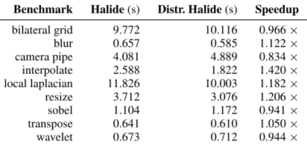
Benchmark Halide (s) Distr. Halide (s) Speedup
bilateral grid 9.772 10.116 0.966 × blur 0.657 0.585 1.122 × camera pipe 4.081 4.889 0.834 × interpolate 2.588 1.822 1.420 × local laplacian 11.826 10.003 1.182 × resize 3.712 3.076 1.206 × sobel 1.104 1.172 0.941 × transpose 0.641 0.610 1.050 × wavelet 0.673 0.712 0.944 ×
Table 6: Runtime and speedup on a single node and the same number of cores with NUMA-aware distribution over two ranks, using each benchmark’s maximum sized input.
Another item of note in the Table 5 is the total number of LLC misses from regular to distributed Halide in this scenario. This is due to the partially static, partially dynamic scheduling that occurs with the distributed schedule. In effect, each rank is statically responsible for the top or bottom half of the rows of the input. Then, parallelization using the dynamic scheduling happens locally over each half. Restricting the domain of parallelism results in better cache utilization on each socket, meaning many of the accesses that missed LLC in regular Halide become hits in higher levels of cache with distributed Halide.
Table 6 summarizes the benefit of using a distributed pipeline to form NUMA-aware static partitions. For each benchmark, we report the runtime of the maximum input size of the regular Halide pipeline versus the distributed pipeline. The distributed pipeline was run on a single node with the same number of cores, but one rank was assigned to each of the two sockets. The numbers are the median runtimes of 50 iterations.
While taking advantage of NUMA could also be done in the parallel runtime, our approach allows the distributed scheduling to generalize to handle NUMA-aware static scheduling, while main-taining the dynamic load balancing already present. This fits within the general Halide philosophy of exposing choices like these as scheduling directives: in effect, the distribute() directive can also become a directive for controlling NUMA-aware partitioning of computation.
5.4 Scalability on Cori
In order to support next-generation large-scale image processing, it is necessary for distributed Halide to scale to much higher core counts, such as what would used for on supercomputer-scale prob-lems. Our testbed machine configuration is not quite representa-tive of typical supercomputer architectures, not least due to the fact that our test network topology is fully connected. To measure how well our results generalize to a real supercomputer, we repeated the scalability measurements on “Cori,” the newest supercomputer available at NERSC [3].
Cori is a Cray XC40 supercomputer, with a theoretical peak per-formance of 1.92 Petaflops/second. It has 1,630 compute nodes to-talling 52,160 cores. Each compute node has two sockets, each of
which is Intel Xeon E5-2698 v3 @ 2.3GHz. The network infras-tructure is Cray Aries, with the “Dragonfly” topology. Each node has 128GB of main memory. More details can be found at [3]. We ran our scalability tests up to a total of 64 nodes, or 2,048 cores.
The findings are summarized in Figure 7. The scalability of the benchmarks is similar to those observed on our testing machine. On 64 nodes, the blur benchmark achieves a 57× speedup for a parallel efficiency of 89%, similar to the 86% efficiency on the 16 node test machine. The benchmarks that exhibited a falloff in scaling on our testing machine (such as local Laplacian) unsurprisingly do not scale on Cori. In the case of interpolate and resize, benchmarks that exhibited decent scaling on our testing machine, the falloff in scalability is due to strong scaling. We were unable to measure a single-node baseline for larger input sizes on these two benchmarks due to memory constraints. Thus, the curves quickly fall off as the limits of useful distribution are reached.
The transpose benchmark appears to display an accelerat-ing scalaccelerat-ing curve on smaller inputs, but these results should be taked with a grain of salt. We included small input sizes up to 20,000×20,000 for consistency across benchmark results, but the absolute difference in execution time between 32 and 64 nodes (1,024 and 2,048 cores) is less than 0.01 seconds, and the baseline is on the order of 0.1 seconds, as reported in Table 6. Thus, the overall effect on execution time is nearly negligible from 32 to 64 nodes.
In general, a larger input size is required to see similar scaling at the 384 core count of our test machine. Most likely this is due to increased network contention during execution. In particular, the compute nodes assigned by the Cori job scheduler are not chosen based on locality, meaning the number of hops required for point-to-point communication can be much larger than on our test machine (which was fully connected). Additionally, Cori is a shared resource, meaning network contention with unrelated jobs could also have a non-negligible impact on scalability of these applications.
6. Related Work
Distributed Scheduling Finding an optimal allocation of tasks to
distributed workers in order to minimize communication is an NP-hard problem in general [14]. As such, there is a wealth of research devoted to approximate algorithms for finding task allocations to minimize communication, e.g. [8, 14, 16, 19, 20, 33]. The dis-tributed Halide compiler does not attempt to automatically deter-mine distributed schedules. This follows the Halide philosophy in allowing the programmer to quickly try many different distributed schedules and empirically arrive at a high-performing distributed schedule. To semi-automate the search process, one can apply an autotuning approach as in [9].
In [15], the authors formulate a static polyhedral analysis al-gorithm to generate efficient communication code for distributed affine loop nests. This work uses a notion of “flow-out inter-section flow-in” sets, derived using polyhedral analysis, to min-imize unnecessary communication present in previous schemes. Our approach of required region intersection is similar to their ap-proach. However, because our code generation can take advantage of domain-specific information available in Halide programs (for example, stencil footprints), our system has additional information that allows our code generation to be much simpler. A more gen-eral approach like flow-out intersection flow-in could be used, but would add unnecessary complexity.
Distributed Languages and Libraries In [23], an edge-detection
benchmark was distributed on a network of workstations. The data partitioning scheme they adopted was to initially distribute all input required by each workstation, meaning no communication was
re-0 500 1000 1500 2000 # cores 0 10 20 30 40 50 60 Speedup 2000x2000 4000x4000 10000x10000 20000x20000 40000x40000 50000x50000 100000x100000 Linear
(a) Bilateral grid
0 500 1000 1500 2000 # cores 0 10 20 30 40 50 60 Speedup 2000x2000 4000x4000 10000x10000 20000x20000 40000x40000 50000x50000 100000x100000 Linear (b) Blur 0 500 1000 1500 2000 # cores 0 10 20 30 40 50 60 Speedup 2000x2000 4000x4000 10000x10000 20000x20000 40000x40000 100000x100000 Linear (c) Camera pipe 0 500 # cores1000 1500 2000 0 10 20 30 40 50 60 Speedup 2000x2000 4000x4000 10000x10000 20000x20000 Linear (d) Interpolate 0 500 # cores1000 1500 2000 0 10 20 30 40 50 60 Speedup 2000x2000 4000x4000 10000x10000 20000x20000 40000x40000 Linear
(e) Local Laplacian
0 500 # cores1000 1500 2000 0 10 20 30 40 50 60 Speedup 2000x2000 4000x4000 10000x10000 20000x20000 Linear (f) Resize 0 500 1000 1500 2000 # cores 0 10 20 30 40 50 60 Speedup 2000x2000 4000x4000 10000x10000 20000x20000 40000x40000 50000x50000 100000x100000 Linear (g) Sobel 0 500 1000 1500 2000 # cores 0 10 20 30 40 50 60 Speedup 2000x2000 4000x4000 10000x10000 20000x20000 40000x40000 50000x50000 100000x100000 Linear (h) Transpose 0 500 1000 1500 2000 # cores 0 10 20 30 40 50 60 Speedup 2000x2000 4000x4000 10000x10000 20000x20000 40000x40000 50000x50000 100000x100000 Linear (i) Wavelet
Figure 7: Scaling results across all benchmarks with varying input sizes on the Cori supercomputer. quired during execution. However, the software architecture in this
work requires the distribution strategy to be implemented on their master workstation, and reimplementing a new data distribution in this architecture requires a non-trivial amount of work.
Some distributed languages such as X10 [11] and Titanium [18] include rich array libraries that allow users to construct distributed multidimensional structured grids, while providing language con-structs that make it easy to communicate ghost zones between neighbors. However, exploring schedules for on-node computation requires rewriting large portions of the code.
DataCutter [10] provides a library approach for automatically communicating data requested by range queries on worker proces-sors. Their approach requires generating an explicit global indexing structure to satisfy the range queries, whereas our approach maps data ranges to owners with simple arithmetic.
Image Processing DSLs Besides Halide, other efforts at building
domain-specific languages for image processing include Forma [30], a DSL by Nvidia for image processing on the GPU and CPU; Dark-room, which compiles image processing pipelines into hardware; and Polymage [25], which implements the subset of Halide for expressing algorithms and uses a model-driven compiler to find a good schedule automatically. None of these implement distributed-memory code generation.
Stencil DSLs Physis [24] takes a compiler approach for
generat-ing distributed stencil codes on heterogeneous clusters. They im-plement a high-level language for expressing stencil code algo-rithms, and their compiler automatically performs optimizations such as overlap of computation and communication. Physis does not have analogy to Halide’s scheduling language, meaning perfor-mance of a distributed stencil code completely depends on the