HAL Id: hal-03120931
https://hal.archives-ouvertes.fr/hal-03120931
Submitted on 26 Jan 2021
HAL is a multi-disciplinary open access
archive for the deposit and dissemination of
sci-entific research documents, whether they are
pub-lished or not. The documents may come from
teaching and research institutions in France or
abroad, or from public or private research centers.
L’archive ouverte pluridisciplinaire HAL, est
destinée au dépôt et à la diffusion de documents
scientifiques de niveau recherche, publiés ou non,
émanant des établissements d’enseignement et de
recherche français ou étrangers, des laboratoires
publics ou privés.
A global database of sea surface dimethylsulfide (DMS)
measurements and a procedure to predict sea surface
DMS as a function of latitude, longitude, and month
A. Kettle, M. Andreae, D. Amouroux, T. Andreae, T. Bates, H. Berresheim,
H. Bingemer, R. Boniforti, M. Curran, G. Ditullio, et al.
To cite this version:
A. Kettle, M. Andreae, D. Amouroux, T. Andreae, T. Bates, et al.. A global database of sea surface
dimethylsulfide (DMS) measurements and a procedure to predict sea surface DMS as a function of
latitude, longitude, and month. Global Biogeochemical Cycles, American Geophysical Union, 1999,
13 (2), pp.399-444. �10.1029/1999GB900004�. �hal-03120931�
GLOBAL BIOGEOCHEMICAL CYCLES, VOL. 13, NO 2, PAGES 399-444, JUNE 1999
A global database of sea surface dimethylsulfide (DMS)
measurements and a procedure to predict sea surface
DMS as a function of latitude, longitude, and month
A. J. Kettle,
• M. O. Andreae,
• D. Amouroux,
•'2
T. W. Andreae,
• T. S. Bates,
3
H. Berresheim,
4 H. B ingemer,
• R. Boniforti,
6 M. A. J. Curran,
7 G. R. DiTullio,
8
G. Helas,
• G. B. Jones,
9 M.D. Keller,
•ø
R. P. Kiene,
• C. Leck,
•2 M. Levasseur,
•
G. Malin,
TM
M. Maspero,
•5
P. Matrai,
•ø
A. R. McTaggart,
•6
N. Mihalopoulos,
•7
B.C. Nguyen,
•8
A. Novo,
•9
J.P. Putaud,
2ø
S. Rapsomanikis,
• G. Roberts,
•
G. Schebeske,
• S. Sharma,
2• R. Sim6,
22
R. Staubes,
5 S. Turner,
TM
and
G. Uher
•'23
Abstract. A database
of 15,617 point measurements
of dimethylsulfide
(DMS) in surface waters
along with lesser amounts
of data for aqueous
and particulate
dirhethylsulfoniopropionate
concentration,
chlorophyll concentration,
sea surface
salinity and temperature,
and wind speed
has been assembled. The database
was processed
to create a series of climatological annual and
monthly
1øxl ø latitude-longitude
squares
of data. The results
were compared
to published
fields
of geophysical
and biological parameters. No significant
correlation
was found between DMS
and these parameters,
and no simple algorithm could be found to create monthly fields of sea
surface
DMS concentration
based on these parameters. Instead, an annual map of sea surface
DMS was produced
using an algorithm similar to that employed by Conkright et al. [1994]. In
this approach,
a first-guess
field of DMS sea surface
concentration
measurements
is created and
then a correction
to this field is generated
based on actual measurements.
Monthly sea surface
grids of DMS were obtained using a similar scheme,
but the sparsity
of DMS measurements
made
the method difficult to implement. A scheme
was used which projected actual data into months
of the year where no data were otherwise
present.
1. Introduction
That dimethylsulfide produced by plankton could change the
radiation budget of the Earth was first proposed by Charlson et
al. [1987]. According to this hypothesis (known by its acronym,
CLAW, after the authors of the publication),
dimethylsulfoniopropionate (DMSP) in phytoplankton cells is *'r, eleased into the water column where it is transformed into
Max Planck Institute for Chemistry, ltogeochemistry Department, Mainz,
Germany.
Laboratorie de Chimie Analytique Bio-Inorganique et Environnement,
Universit6 de Pau et des Pays de I'Adour, France,
NOAA/Pacific Marine Environmental Laboratory, Seattle, Washington.
DWD/MOHp, Hohenpeissenberg, Germany.
Johann Wolfgang Goethe University, Frankfurt am Main, Germany. ENEA Centro Ricerthe Ambiente Marino, La Spezia, Italy.
Antarctic CRC and Australian Antarctic Division, University of Taanania,
Hobart, Tasmania, Australia.
University of Charleston, Grice Marine Laboratory, Charleston, South
Carolina.
James Cook University of North Queensland, Townsville, Queensland,
Australia.
Copyright 1999 by the American Geophysical Union.
Paper number 1999GB900004.
0886-6236/99/1999GB900004512.00
dimethylsulfide (DMS). DMS diffuses through the sea surface to
the atmosphere where it is oxidized to SO2 and methane sulfonic acid (MSA). SO2 can be oxidized to H2SO4, which can then
form sulfate
particles,
that may alter the radiation
budget
of the
Earth through
modification
of cloud optical properties. This
could cool down the temperature of the upper ocean and might
change the metabolism and speciation of plankton [Lawrence,
1993], which in turn could modify the emission of DMS to the
•øBigelow Laboratory of Ocean Sciences, McKown Point, West Boothbay
Harbor, Maine.
'•Department of Marine Sciences, University of South Alabama, Mobile,
Alabama.
UDepartment of Meteorology, Stockholm University, Stockholm, Sweden.
•3Institut Mauriee-Lamontagne, Minist•re des P•ehes et des Oe6ans,
Mont-Joli, Qu6bec, Canada.
•4University of East Anglia, Norwich, England. •CISE SpA, Milano, Italy
•6Australia Antarctic Division, Kingston, Tasmania, Australia. •7Universityof Crete, Iraklion, Crete, Greece.
•SCentre des Faibles Radioactivit6s, Laboratoire mixte CNRS-CEA, Avenue de la Terrasse, Gif-Sur-Yvettte Cedex, France.
•gENEL-CRAM, Milano, Italy.
•øJoint Research Centre, Ispra, Italy.
UAtmospheric Environment Service, Downsview, Ontario, Canada. 22Institue de Cieneies del March, Barcelona, Catalonia, Spain.
2•Universiity of Newcastle upon Tyne, Ridley Building, Newscastle upon Tyne, England.
400 KETTLE ET AL.: SEA SURFACE DIMETHYLSULFIDE MEASUREMENTS
atmosphere. This feedback cycle was hypothesized to modify
global climate, and if the overall sign of the feedback is negative,
it would act to counter greenhouse warming. In addition to the
study of Charlson et al. [1987], other investigators have also
considered the linkages between DMS and climate [Shaw, 1983;
Schwartz, 1988; Foley et al., 1991; Lawrence, 1993; Shaw et al.,
1996]. However, the processes that govern each step in the
hypothesis remain poorly understood and are the subject of
continuing investigations [Andreae and Crutzen, 1997].
Because the rate of aerosol production.•from marine DMS can
be influenced by climatic feedbacks [Andreae and Crutzen,
1997], there has been extensive work on the processes that
control the production of DMS and its precursors, its emission
and oxidation in the atmosphere, and the parameterization of the
effect of the resultant sulfate particles on the radiation budget.
The parameterization of the DMSP production and release
processes within a plankton community is of particular interest,
and the ultimate goal is to understand this process well enough to
predict both the generation and destruction of DMS in the upper
ocean as a function of latitude, longitude, and time.
The first measurements of DMS were made by Lovelock et
al. [1972], followed by Nguyen et al. [1978], Andreae and
Raemdonck [1983], Cline and Bates [1983], Bingemer [1984], Turner and Liss [1985], Berresheim [1987], Leck et al. [1990], and many other research groups in more recent times. It is
known that DMS is a hydrolysis product of
dimethylsulfoniopropionate (DMSP), a compound produced by
phytoplankton possibly for cellular osmotic regulation [Kirst et
al., 1991] or cryoprotection [Karsten et al., 1992]. There have
been many studies which found correlations between DMS and
chlorophyll a (chl a) concentration [Andreae and Barnard, 1984;
Turner et al., 1988, 1989; Malin et al., 1993, 1994; Uchida et al., 1992; McTaggart and Burton, 1993; Liss et al., 1994] or
phytoplankton cell concentration [Biirgermeister et al., 1990;
Barnard et al., 1984; Holligan et al., 1987; Gibson et al., 1988, 1990]. Other studies have observed correlations between DMSP
and chlorophyll a concentration [Malin et al., 1993, 1994;
Curran et al., 1998]. These relationships were thought to hold
much promise for being able to deduce the DMS flux from
satellite or airborne remote determinations of chlorophyll concentration [Thompson et al., 1990; Matrai et al., 1993; Gabric et al., 1995, 1996].
On the other hand, there have also been studies where no
correlation was found with either phytoplankton cell number
[Leck et al., 1990] or chlorophyll concentration [Andreae and
Barnard, 1984; Holligan et al., 1987; Watanabe et al., 1995a] on
larger regional scales. This has several possible explanations.
First, populations of phytoplankton are not homogeneous in the
ocean, and second, different species of phytoplankton contain
different amounts of DMSP [Keller et al., 1989] and different
concentrations and types of chlorophyll [Sathyendranath et al.,
1987]. Groene [1995] states that in most cases wherein there was a high correlation between DMS and chlorophyll
concentration, one species of phytoplankton dominated the
bloom. As well, even though DMS is produced by
phytoplankton,
it is released to the water column by
phytoplankton
and zooplankton
excretion, by phytoplankton
senescence [Nguyen et al., 1990; Kwint et al., 1995], by
zooplankton
grazing
[Dacey
and Wakeham,
1986; Belviso
et al.,
1990; Cantin et al., 1996], and possibly by viral infection [Malin
et al., 1992; Bratbak et al., 1995]. In addition, DMS is subject
to a number of removal mechanisms including bacterial and
photochemical degradation [Kiene and Bates, 1990], surface
outgassing, and downward mixing that vary according to time,
place, and meteorological conditions [Andreae and Crutzen,
1997]. One can therefore not necessarily expect a simple
correlation between DMS and phytoplankton cell number or
chlorophyll concentration.
Bates et al. [1987a, 1988] proposed that latitudinally averaged concentrations of DMS flux should correlate with average light intensities or latitude. The idea that DMS sea surface concentration may be associated with light has some support in the fact that the phytoplankton, which produces DMS, grows over a period of days as the result of carbon assimilation through photosynthesis. This was investigated in laboratory experiments [Karsten et al., 1991; Vetter and Sharp, 1993; Crocker et al., 1995; Matrai et al., 1995]. Other researchers have
proposed a correlation between DMS concentrations and primary
production or the time rate of change of phytoplankton
concentration [Andreae and Raemdonck, 1983; Andreae and
Barnard, 1984; Andreae, 1986; McTaggart and Burton, 1993].
Although Matrai et al. [1993] do not find a relationship between
DMS and primary productivity, the proposed correlation could
still hold some promise for global modeling given recent attempts to deduce in situ primary production from satellite measurements [Platt et al., 1995; Longhurst et al., 1995; Sathyendranath et al., 1995], subject to the limitations identified by Balch et al. [1992]. There have also been attempts to find correlations between DMS and other in situ measurements. The relation with salinity was recognized relatively early in DMS investigations [Reed, 1983; Froelich et al., 1985; Vairavamurthy et al., 1985; Iverson et al., 1989] and formed the basis of the hypothesis that DMSP is used by phytoplankton as an osmoregulator. This correlation showed promise for global modelers because of the existence of globally gridded fields of salinity already in existence [Levitus et al., 1994]. However, other field studies have not found strong correlations between DMS and salinity [Leck and Rodhe, 1991], and even if a strong correlation were found, the salinity of the
open ocean is homogeneous enough that a DMS sea surface
concentration parameterization would not be useful. McTaggart and Burton [1993] reported a negative correlation between DMS and in situ temperatures on the coast of the Antarctica in the austral summer, and this has formed the basis of a hypothesis
that DMSP may function as a cryoprotector within phytoplankton
cells. However, Leck et al. [1990] reported a positive correlation between DMS and annual in situ temperature for a coastal site in the Baltic Sea, and it therefore seems unlikely that DMS sea surface concentrations can be determined from the global
temperature field. Andreae [1986] hypothesized that a
relationship between DMSP and dissolved nitrate could occur
under conditions of nitrate limitation when DMSP is used as a
substitute for the nitrogen-containing compounds glycine betaine and proline in cell functions. This hypothesis was supported by the results of Leck et al. [1990] and Curran et al. [1998] (who reported a negative correlation between dissolved nitrate and DMSP in a field study) and also by the laboratory results of Keller and Bellows [1996]. The correlations between DMS and nutrients have generally not been high enough to allow existing gridded nutrient fields to act as a basis to create a series of DMS
maps.
There have been some process models developed recently which show more promise than the simple models based on
KETrLE ET AL.: SEA SURFACE DIMETHYLSULFIDE MEASUREMENTS 401
correlations. Murray et al. [1992] developed the first of these by
incorporating mechanisms of DMS and DMSP production and
destruction into a simple ecosystem model incorporating dissolved inorganic nitrogen, phytoplankton, bacteria, zooflagellates, large protozoa, and macrozooplankton. One interesting result of this mathematical model is that DMS concentration should increase a few days after a phytoplankton bloom so that there should be an (imperfect) correlation between DMS and phytoplankton concentration (the exact results depend
on the values of the constants chosen in this nonlinear model).
This result was actually observed in field and laboratory studies [Nguyen et al., 1988; Matrai and Keller, 1993]. Gabric et al.
[1993a, b] give a further elaboration of this same model without
applying it to a particular geophysical data set, and Gabric et al.
[1995] apply it to the Southern Ocean south of Australia,
incorporating as much as possible of meteorological forcing to
drive the biological model. This application of the ecosystem model predicted periodic spikes in the chlorophyll and DMS concentrations with a period of about 30 days. This behavior has not been reported in extended measurements of ecosystems made up to this point [Leck et al., 1990; Dacey et al., 1996].
Recently, van der Berg et al. [1996] successfully coupled a
DMS production
model
with an ecosys,
tem model
driven
by
physical forcing mechanisms. The coupled model was used to
simulate the annual evolution of DMS sea surface concentration
and flux in the North Sea and gave insight into the chemical and biological processes which govern DMS concentration in this
water body. Specifically, the enzyme DMSP lyase was
identified as an important factor in the conversion of DMSP to DMS than bacteria. As well, the modeling study highlighted the
importance of Phaeocystis populations as reservoirs of DMSP
and the fact that these populations are mainly not grazed by zooplankton. Thus, at least for the North Sea, bacteria and zooplankton seem to play a subordinate role in governing the
DMS concentration in the water column.
Given the complex situation described in the previous
paragraphs, the task of making maps of DMS concentration
seems difficult, but there is a precedent for mapping other biogeochemically relevant species in the ocean [Conkright et al.,
1994; Nevison et al., 1995]. To make any map based on
geophysical data, one needs point measurements and a scheme to
extrapolate the measurements to a gridded field, in this case, the
globe. Thus, the first step in the creation of any map is the
assembly of a data base of existing measurements. For example,
Levitus and Boyer [1994a] used a database of 279,239
measurements of sea surface oxygen concentration to create a
seasonal climatological map at løxlø latitude-longitude
resolution, The basis of their map is a latitudinal average of
concentrations taken in an ocean basin and the subsequent calculation of the discrepancy between this background average
value and the actual point measurement using a distance-
weighted average scheme. Conkright et al. [1994] used the same
scheme to create global annual average maps of nitrate,
phosphate,
and silicate
concentration
with a database
of 61,817,
171,064, and 80,235 surface measurements, respectively.
In contrast to these studies, previous mapping attempts for
sea surface DMS have been relatively simple and hindered by the
sparsity of data. For example, Erickson et al. [1990] used the
assumption of Bates et al. [1987a] that DMS ocean fluxes vary
with surface irradiance intensity to calculate the global field of
sea surface DMS concentrations. This was a first attempt to
model DMS concentrations on a global scale, and it made the interesting prediction that the highest surface concentrations would occur at the highest latitudes. This was subsequently substantiated in numerous measurement expeditions both to the Arctic and Antarctic regions (see Table 1 and Figure 1). On the other hand, this model could not account for the observed strong
longitudinal gradients in DMS concentration [Andreae et al.,
1994]. Spiro et al. [1992] used the work of Bates et al. [1987a] to parameterize the oceanic contribution to DMS flux in creating
a series of 1øxl ø monthly maps of sulfur emissions. Galloway et
al. [1992] pooled much of the data for the North Atlantic Ocean and prescribed a scheme for the monthly variation of DMS sea surface concentration for coastal and deep ocean sites.
Liss et al. [1993] and Turner et al. [1996a] created a series of nine monthly maps of sea surface DMS distribution in the North Sea. The interpolation method used is not mentioned, but the network of measurements is quite dense. Tarrasdn et al. [1995]
combined the approach of Galloway et al. [1992] and Liss et al.
[1993] to develop a scheme where the North Atlantic Ocean was divided into three oceanographically similar areas (deep water and coastal sites and the North Sea as its own region) with monthly climatology to model the annual DMS flux and its contribution to sulfate aerosol levels over Europe. Turner et al. [1995] developed a similar scheme of monthly climatology for the Southern Ocean. They thus prescribed how DMS sea surface concentration should vary over an annual cycle over a large
region of the ocean. This seems to be a poor substitute for a fully
predictive model that can simulate plankton population dynamics and have applicability to the global ocean. However, it is otherwise difficult to map global sea surface DMS concentrations
because there are not many more than 15,000 measurements in
existence, and there is limited knowledge of how DMS
concentrations vary in the global ocean.
The aim of this paper is to present the results of the largest global database of sea surface measurements of DMS assembled
up to now. The database will be summarized, and a climatology
of the results will be presented and compared with climatological summaries of other biogeochemical, oceanographic, and meteorological parameters. Finally, a procedure will be proposed to predict the monthly sea surface concentrations of DMS. Because of the temporal and spatial variability of DMS concentrations, the procedure attempts to generate monthly maps
of DMS based on the biogeochemical scheme proposed by
Longhurst et al. [ 1995].
We intend to derive emission estimates based on the
concentration fields presented here and to include our results into the set of maps of chemical emissions both from oceans and land surfaces produced as part of the Global Emissions Inventory Activity-International Global Atmospheric Chemistry (GEIA- IGAC) project. These have been reported by Graedel et al. [1993] and Graedel [1994], and the latest information about the
gridded data sets available through the GEIA project is available
from the Internet at
h ttp ://b lueskies. sprl. umich. edu/geia/index. h tml.
2. Methods
The center of the project is a database of 15,617 DMS measurements which were contributed by scientists or digitized
from publications (Plate 1 and Table 1). This project was
404 KETTLE ET AL.: SEA SURFACE DIMETHYLSULFIDE MEASUREMENTS
406
KETTLE ET AL.' SEA SURFACE
DIMETHYLSULFIDE
MEASUREMENTS
•
0
0 •
o
• o • 8
o
•
o • o
_
•
....
•
•
KET'FLE ET AL.: SEA SURFACE DIMETHYLSULFIDE MEASUREMENTS 407
on Biogeochemical Ocean-Atmosphere Transfers (BOAT) held
in Bermuda 1992. It was suggested that the database be
constructed from data contributions by individual scientists and
that the completed database be made available to the scientific community. In addition to sea surface DMS concentration
measurements, further information was requested about
measurements
of aqueous
DMSP, particulate
DMSP, chlorophyll
a concentration, wind speed, sea surface temperature, sea surface
salinity, primary productivity, and total water depth.
Information
was also requested
about the time of sampling,
the
latitude and longitude of the sample, the depth at which the water
samples
were taken, and whether
or not the seawater
samples
were filtered before analysis. The contributions by scientists
make up more than 90% of the current DMS data set. The rest of
the data was obtained
through a combination
of digitizing
information
directly from publications
and contacting
the
research ship operators for information about ship cruise tracks
and meteorological parameters. A summary of all the contributed
and digitized data sets is given in Table 1.
In addition to the data contributed as part of the database, an
attempt was made to draw together as much biogeochemical and
geophysical climatological data as possible to assist in the
interpretation
of the data.
The monthly climatological
information
about
sea surface
temperature,
salinity,
oxygen,
and
nutrients came from the World Ocean Atlas (WOA) of Levitus
and Boyer [1994a], Levitus et al. [1994], Levitus and Boyer
[1994b], and Conkright et al. [1994], respectively. All of this
information
has been published
at 1øxl
ø latitude-longitude
resolution. Information
about climatological
wind speeds
was
obtained
from the global wind stress climatology
based on
European Centre for Medium Range Weather Forecasts
(ECMWF) analysis performed by Trenberth et al. [1989]. This
information
is provided
at 2.5øx2.5
ø latitude-longitude
resolution
and is interpolated
to 1øxl
ø latitude-longitude
resolution
for use
in this work. The climatology for the daily average insolation for
a given month was calculated from the daily average insolation
provided
by Bishop
and Rossow
[1991] from July 1, 1983 to June
30, 1991. This data set was also provided at 2.5øx2.5 ø latitude-
longitude
resolution
and interpolated
to 1øxl
ø latitude-longitude
resolution
for use in this work. The mixed layer depth was
obtained from the Samuels and Cox' Geophysical
Fluid
Dynamics Laboratory (GFDL) Global Oceanographic Data Set
Atlas obtained from National Center for Atmospheric Research (NCAR). The climatological, interpolated Coastal Zone Coastal Scanner (CZCS) chlorophyll concentrations were obtained as an unpublished data set from Carmen M. Benkovitz, Richard Wagener, and Gail Elefanio in the Department of Applied Science at Brookhaven National Laboratory. The ocean depth
data was obtained from the NGDC ETOPO5 Global Ocean Depth
and Land Elevation [National Geophysical Data Center (NGDC),
1988]. The data set is provided at 5-min latitude-longitude
resolution, and the water depths at the points of the DMS sea surface measurements are calculated using a distance-weighted averaging scheme. The climatology for the sea ice cover in the northern and southern hemispheres was calculated from the time series data set compiled by Bill Chapman, Department of Atmospheric Sciences, University of Illinois and obtained from
the Internet in 1996. These data were given in polar coordinates
and was interpolated
or averaged
to the 1øxl
ø latitude-longitude
grid used in this study.
408 KETI'LE ET AL.: SEA SURFACE DIMETHYLSULFIDE MEASUREMENTS
z z z o ul • (D ©
o o o o o o
KETTLE ET AL.' SEA SURFACE DIMETHYLSULFIDE MEASUREMENTS 409 o o z• z oPnt!to9
410 KETI'LE ET AL.: SEA SURFACE DIMETHYLSULFIDE MEASUREMENTS
:3
o.• iZ
KETTLE ET AL.' SEA SURFACE DIMETHYLSULFIDE MEASUREMENTS 411
z z z o • • •
412 KETFLE ET AL.' SEA SURFACE DIMETHYLSULFIDE MEASUREMENTS •_9 IOUaU I ß i,i i,i
'"" '""" " : • .'C"
2.. ,,"
d" . ..:- , - •I. - ' .. -- . ,m P ..,,... ,. ,.%• .- .,• . -..,..:
'1
o
•._...
•'r"- ._
' -L---.."-i•
'=.
!
o
-
..
I,!
'"" ,. ...
..
-- "-"' ' ' ....
":
...
•'"-'
0
Z Z Z 0 {.t3 {.t3 1,1300 0 0 0 0 0 0 epnH•r•9KETYLE ET AL.: SEA SURFACE DIMETHYLSULFIDE MEASUREMENTS 413
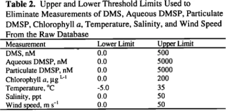
Table 2. Upper and Lower Threshold Limits Used to
Eliminate Measurements of DMS, Aqueous DMSP, Particulate
DMSP, Chlorophyll a, Temperature, Salinity, and Wind Speed
From the Raw Database
Measurement Lower Limit Upper Limit
DMS, nM 0.0 500 Aqueous DMSP, nM 0.0 5000 Particulate DMSP, nM 0.0 5000 Chlorophyll a, gg t.-i 0.0 200 Temperature, øC -5.0 35 Salinity, ppt 0.0 50
Wind
speed,
m s
-l
0.0
50
FORTRAN software. Several analyses were performed. For the
simple statistical analysis, the raw contributed data was subjected to a rigorous filtering process to remove points that contained
known errors or were inconsistent with other measurements. For
example, Curran et al. [1998] reported that in a number of studies wherein water samples were treated with HgC12, the resultant DMS concentrations were higher than whose measured in situ, owing to the conversion of DMSP to DMS. This throws some doubt on the absolute concentrations reported by Deprez et al. [1986], Gibson et al. [1990], McTaggart and Burton [1992], and Crocker et al. [1995], and data contributions 39 and 54 (from Table 1, 58 points) were discarded in this investigation for that reason. In addition, data set 44 (21 points) was not used because its values were feared to be anomalously high. This set is not really significant except for the fact that most of the Australian
data occurs in a sector of the Southern Ocean which does not
have a high data density. Similarly, the data of Lovelock
[Lovelock et al., 1972; Liss et al., 1997] (data set 1, 20 points)
could not be used because the values were about an order of
magnitude too low in comparison t6 later measurements in the Atlantic Ocean. This discrepancy was also reported by Nguyen et al. [ 1978].
Two analyses were performed that led to the creation of sea surface maps of [DMS]: one using the scheme of Conkright et al. [1994] to create a single map of annual sea surface [DMS] and
a second depending on a scheme of biogeochemical provinces to
create a set of monthly maps of sea surface [DMS]. The data cleaning procedure used for each analysis was the same. Points
from the database were flagged for elimination if they fell outside
certain broad threshold limits (given in Table 2). Although it
was difficult to establish an absolute criterion for the chemical
parameters (DMS and DMSP), variables such as temperature and salinity are physically constrained within certain limits, and data outside these limits were flagged and discarded. After this, a statistical checking procedure was implemented whereby the data
in the database were divided up into monthly 5øx5 ø squares. For
each square, a mean and the standard deviation was calculated. Then, each point in the square was compared with the mean, and
if it fell outside of 4.5 standard deviations of the mean, it was
discarded. (This standard deviation threshold was chosen in the
data selection process after systematic trials for values between 3
and 5 standard deviations revealed a discontinuity in the number
of discarded points at the 4.5 standard deviation factor.) The
mean and the standard deviation were then recalculated, and the
selection process was repeated. The iteration was repeated until
no further points failed the standard deviation test. In most cases this was satisfied by one or two runs, although in one case seven
iterations were made before no more points were discarded. At
any time, if there were fewer than four points in the square, then the iteration/elimination procedure was stopped, and the remaining points were retained. At the end, this left a database cleaned of outlying points, leaving 14,980 good data points from the starting number of 15,617.
An annual climatology was next created by dividing these
data points
into a global
grid of 1øxl
ø squares. The DMS pixel
value was taken to be the average of all the individual
measurements within the 1 ø square. If there was only one
measurement within the 1 ø square, the pixel value was taken as
the value of the single measurement. Altogether there were 3317 annual climatological pixels formed from the database. These climatological [DMS] data were compared by regression analysis to literature fields of nitrate, silicate, phosphate, oxygen, and bathymetry (where only a single annual gridded field was available) and also to climatological quantities of aqueous and particulate DMSP, chlorophyll concentration, wind speed, salinity, and temperature (all calculated from contributions to the database using the same cleaning procedure as for [DMS]).
To form a first-guess global field of sea surface [DMS], the climatological pixels were divided into the series of 57 oceanic biogeochemical provinces formulated by Longhurst et al. [1995] to calculate global primary production..The average [DMS] of each province was calculated, and in those few instances where no data pixels were found in a given climatological province, the average [DMS] from an adjacent province was taken. Then, an unweighted 11-point filter was used to smooth the discontinuities at the borders between provinces to create a first-guess field. A correction to the first guess-field was formulated by first subtracting the first-guess field from the average DMS value in the series of ocean data squares, and then applying the same distance-weighted interpolation scheme used by Conkright et al. [1994] to create annual nutrient maps. The correction field was added to the first-guess field, and the sum was smoothed by a five-point median filter used by Conkright et al. [1994], followed by an 11-point unweighted smoothing filter (the Shuman [1957] smoothing filter created artificially steep gradients with this data set). This scheme constitutes the first step in the method of successive corrections described by Daley [1991]. The DMS objective analysis procedure was stopped after the first iteration following the approach of Conkright et al. [1994].
Formulation of the series of monthly global maps of climatological [DMS] was difficult because there were not enough data points to calculate climatological pixel values. The
4331 1 o ocean
data squares
calculated
for the annual
[DMS] field
were much fewer than the 9170 used by Conkright et al. [1994]
to formulate an annual nitrate field. Nevertheless, the same
data-cleaning procedure used for the annual sea surface
concentration field was used here. In the end, the ocean data
squares were divided by month instead of being kept on the
single annual pattern. The procedure was repeated for all the quantities in the database: DMS, aqueous DMSP, particulate DMSP, chlorophyll concentration, wind speed, and sea surface
temperature and salinity. These climatological quantities were
then compared to published values of monthly sea surface
414 KETTLE ET AL.: SEA SURFACE DIMETHYLSULFIDE MEASUREMENTS
chlorophyll concentration, actual surface irradiance, theoretical clear sky irradiance (i.e., calculated irradiance in the absence of clouds), and surface wind speeds.
The first-guess fields were formulated in the same manner as in the creation of the annual climatological map. The monthly average pixels (ocean data squares) were distributed among the
series of 57 biogeochemical provinces formulated by Longhurst
et al. [1995] and average monthly [DMS] quantities were
calculated for each province. The problem of data sparsity was
worse in this monthly case than in the annual case because the
data density was diluted 12-fold. The temporal distribution of
data in some provinces was sufficient to construct an annual pattern of DMS concentrations by connecting the existing points
with a spline construction. In many cases, the temporal
distribution of data was not sufficient to construct a clear annual
cycle, and in these cases the annual trends of [DMS] were taken from other provinces which had a better data set and were considered to be biogeographically similar. Sometimes the fitted spline construction was scaled to minimize the sum of the square
of the differences with the data. The exact nature of the substitutions which were made is summarized in Table 3.
In this way a series of monthly grids of DMS concentration
were created. Following the procedure used for the annual map,
the discontinuities between the boundaries of the biogeochemical provinces were smoothed by the application of an 1' 1-point filter.
This became the first-guess DMS concentration field. An
attempt was made to assimilate the ocean data squares into this first-guess concentration field to create a more realistic map. This created a good result in areas where there was high data density and good temporal coverage, e.g., the northeast 'Atlantic Ocean. However, for the most part, there were not enough ocean data squares in each monthly map to have a significant effect.
An analysis scheme was developed which attempted a
temporal interpolation in those biogeochemical provinces where
there was a higher data density. In this procedure, the monthly time series of data in individual ocean data squares was isolated. These pixels were then used to interpolate to those monthly
pixels where there was no data. The template used for the
interpolation was the same as that used for the larger
biogeochemical province, scaled for the individual ocean data
square according to the values of the data within the pixel. Because of the nature of this assumption, the procedure was only conducted for those biogeochemical provinces where there was sufficient data to determine a template of annual variation. This was defined from Table'3 to include only those biogeochemical provinces where the shape substitute in column 2 and the province in column 1 match. For those other areas which did not have enough data to define an annual template, the actual data from the database was incorporated, but no attempt at interpolation was made. Next, the interpolation and smoothing scheme used in the annual map abox•e was used to create a series
of 12 monthly maps of sea surface DMS concentration.
The question of establishing a confidence interval on the stated value of DMS concentration is not easy to answer. Ideally, one would assess both the accuracy and precision associated with both the annual and monthly climatological DMS maps. Estimating the precision of DMS values for a given pixel would involve assessing the standard deviation of the point DMS measurements in that pixel. This would require many more point measurements of DMS than are actually available. In the
absence of a larger database of DMS measurements, the precision
of the maps was estimated by finding the standard deviation of
all the point measurements found within the radius of 555 km of
an analyzed ocean pixel. This was performed for both the annual
and monthly climatological data sets.
Estimating the accuracy of the entire mapping algorithm used
to generate the interpolated DMS maps was also difficult because
there is no a priori knowledge of the true monthly DMS
concentration field which one could use to assess the
effectiveness of the procedure. There is no precedent for using
this particular mapping method, and consequently no estimates of
the kind of uncertainty involved. To estimate the uncertainty in
the mapping algorithm for the annual climatological grid, the
entire procedure was repeated for fields for which maps have
already been created based on a large database of measurements:
nitrate, silicate, phosphate, and oxygen from the World Ocean
Atlas and the annually averaged CZCS chlorophyll field. Data
were extracted from these fields at the same location as the 1øxl ø
ocean data squares for DMS, and this was then used to calculate
annual average values for each biogeochemical province. These
fields were smoothed, and data were assimilated in the same
manner as for DMS. Then the absolute value of the difference
was found between the new annual map created with the sparse
data set and the published map. This calculated difference field
was divided by the standard deviation of the published field to
make it comparable with other data sets. Then, the average of
the five dimensionless difference fields was calculated. This
represents a average error field in reproducing published annual
maps using the mapping algorithm of this paper. This error field
was next scaled by the standard deviation of the annual DMS
field. If DMS is distributed in the same manner as the other
published annual quantities (which is not unreasonable for
chlorophyll and the nutrients), then this would be a reasonable
uncertainty associated with the annual DMS map. For the
monthly DMS maps, a similar procedure was applied except that
the single set of monthly fields of CZCS chlorophyll
concentration was employed instead.
3. Results
The location of the sea surface DMS concentration
information is presented in Figure l a. Figures lb, l c, and l d
present the location of sea surface concentrations of aqueous
DMSP, particulate DMSP, and chlorophyll a, respectively. The
data contributions are number coded to correspond with the
information • in Table 1. Figure 1 a illustrates that the distribution
of DMS measurements is global with the highest coverage in the
North Atlantic, North Pacific, and Southern Oceans, and the lowest coverage in the Indian and southwest Pacific Oceans.
Altogether, there are 15,617 DMS measurements plotted on this
map.
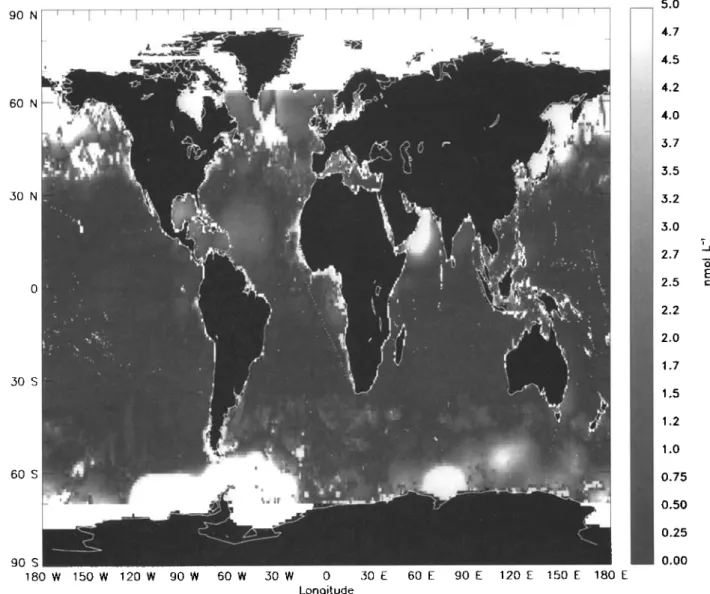
These points were cleaned according to the procedures given
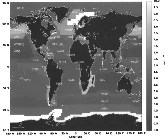
in the methods section and then binned into 3317 1øxl ø ocean
data squares. The map of these pixels is shown in Plate 1. All
annual variation of DMS concentration is lost in this map, but it is still interesting because it shows that DMS concentrations over much of the oceans are low. The highest concentrations are in
some coastal upwelling areas (North Africa, Peru, Angola, and
the equatorial Pacific Ocean), and in the high-latitude regions of
KETTLE ET AL.: SEA SURFACE DIMETHYLSULFIDE MEASUREMENTS 415
Table 3: Scheme of Substitutions for the Monthly
Province
First-Guess Field of DMS Concentration
Shape Phase Shift Scaling Number of
Substitute Months
Boreal Polar (BPLR) Atlantic Arctic (ARCT) Atlantic Subarctic (SARC) North Atlantic Drift (NADR) Gulf Stream (GFST)
North Atlantic Subtropical Gyral- West (NAST-W) North Atlantic Tropical Gyral (NATR)
Western Tropical Atlantic (WTRA) Eastern Tropical Atlantic (ETRA) South Atlantic Gyral (SATL)
North-East Atlantic Shelves (NECS)
Canary Coastal (CNRY)
Guinea Current Coastal (GUIN) Guianas Coastal (GUIA)
North-West Atlantic Shelves (NWCS) Mediterranean Sea- Black Sea (MEDI) Caribbean (CARB)
North Atlantic Subtropical Gyral - East (NAST-E) Chesapeake Bay (CHSB)
Brazil Current Coastal (BRAZ) South-West Atlantic Shelves (FKLD)
Benguela Current Coastal (BENG) Indian Monsoon Gyres (MONS) Indian South Subtropical Gyre (ISSG)
East Africa Coastal (EAFR) Red Sea, Persian Gulf (REDS) North-West Arabian Upwelling (ARAB) East India Coastal (INDE)
West India Coastal (INDW) Australia-Indonesia Coastal (AUSW)
North Pacific Epicontinental (BERS) Pacific Subarctic Gyres - East (PSAG-E) Pacific Subarctic Gyres - West (PSAG-W)
Kuroshio Current (KURO) North Pacific Polar Front (NPPF)
North Pacific Subtropical Gyre - East (NPST-E) North Pacific Subtropical Gyre - West (NPST-W)
Offshore California Current (OCAL) Tasman Sea (TASM)
South Pacific Subtropical Gyre (SPSG)
North Pacific Tropical Gyre (NPTG)
North Pacific Equatorial Countercurrent (PNEC) Pacific Equatorial Divergence (PEQD)
West Pacific Warm Pool (WARM)
Archipelagic Deep Basins (ARCH) Alaska Downwelling Coastal (ALSK) California Upwelling Coastal (CCAL)
Central American Coastal (CAMR) Chile-Peru Current Coastal (CHIL) China Sea Coastal (CHIN) Sunda-Arafura Shelves (SUND) East Australian Coastal (AUSE) New Zealand Coastal (NEWZ)
South Subtropical Convergence (SSTC)
Subantarctic (SANT) Antarctic (ANTA) Austral Polar (APLR)
BPLR n n 6 ARCT n n 5 NADR n n 4 NADR n n 7 NAST-W n y 6 NAST-W n n 11 NATR n n 8 ETRA n y 7 ETRA n n 6 SSTC n y 8 NECS n y 12 CNRY n n 5 ETRA n n 2 ETRA n y 2 NWCS n n 11 MEDI n n 8 CARB n n 11 NAST-E n n 8 NWCS n y 2 SATL n y 4 SSTC n y 4 SATL n y 3 MONS n n 3 SSTC n n 2 SATL n n 1 ARAB n y l ARAB n n 4 ARAB n n 0 ARAB n n 0 SATL n n 1 NECS n y 4 NAST-W n y 4 NADR n n 0 KURO n n 5 NPPF n y 4 NPST-E n n 5 NPST-E n n 2 OCAL n y 6 TASM n y 4 SSTC n n 7 NPTG n y 10 PNEC n n 7 PEQD n n 9 PNEC n n 4 note I n n 3 NECS n y 2 CCAL n n 7 CCAL n n 1 PEQD n y 2 CHIN n n 9 note 1 n n 2 TASM n n 2 SSTC n n 0 SSTC n y 12 ANTA n y 8 ANTA n y 8 APLR n y 8
Phase shift refers to a six month phase shift in those cases where a pattern from the southern hemisphere was used to characterize the annual cycle of DMS concentration in the northern hemisphere. Scaling refers to the adjustment of the spline construction so as to minimize the sum of the squares of the differences between the spline curve and the actual data. Note 1: the shape of the annual DMS cycle in these provinces was constructed by combining data from PNEC and PEQD without subsequent scaling.
416 KETYLE ET AL.: SEA SURFACE DIMETHYLSULFIDE MEASUREMENTS 1 [ , I • • , • 1 0 0 0 tO) I I ... I ... [ I t__ 1 [ ... i ... i ... t ... i , , ,! .... 0 0 0 0 0 0 "-" b") El_ o• o ' o o ' i • i i • i i • i I i I i , , i i • i 0 o 1 i ... i ... i ... I , ! ... 0 0 0 0 0 0 0 0 '' 0 0 h i i • i i 0 0 0 t.• 0 t.• I I , , , , i o o Lt') 0 J ! , , [ •J , , I lj --j i , i I --1 i i i l L--• o m n o o& o o •E o& ._
KETTLE ET AL.: SEA SURFACE DIMETHYLSULFIDE MEASUREMENTS 417
Table 4. Annual
Statistical
Quantities
for the Parameters
in the Database
and for Analogous
Parameters
Taken From the World
Ocean AtlasQuantity Mean Median Standard Geometric Geometric Minimum Maximum N
Deviation Mean Standard
Deviation
Database DMS, nM 5.52 2.22 20.55 2.35 2.74 0.04 315.69 3382
Database aqueous DMSP, nM 16.91 9.76 22.17 8.97 3.38 0.13 198.50 578
Database particulate DMSP, nM 43.61 22.39 53.66 23.65 3.11 1.04 325.32 662
Database
chlorophyll,
lagL
q
1.092
0.427
2.235
0.414
4.010
0.016
29.136
1286
Database wind speed, ms q 7.94 7.49 3.81 7.011 1.698 0.09 29.00 2367
Database salinity, ppt 34.18 34.48 3.34 33.82 1.20 3.34 37.60 1391
Database temperature, øC 17.30 19.75 10.29 N/A N/A -4.44 32.15 2883
WOA
nitrate,
laM
5.078
1.757
7.000
2.062
4.073
0.0002
28.864
3282
WOA
silicate,
laM
0.538
0.373
0.481
0.368
2.425
0.004
1.867
3282
WOA
phosphorus,
laM
9.198
3.909
14.292
4.971
2.594
0.634
70.350
3282
WOA oxygen, rnL/L 5.798 5.383 1.234 5.676 1.224 4.004 9.278 3282
ETOPO5
Depth,
m
3381
3960
1729
2205
4
0.625
5970
3175
ETOPO5 refers to depth information taken from the National Geophysical Data Center [1988].
DMS concentrations, but there are patches of high DMS
scattered throughout the oceans.
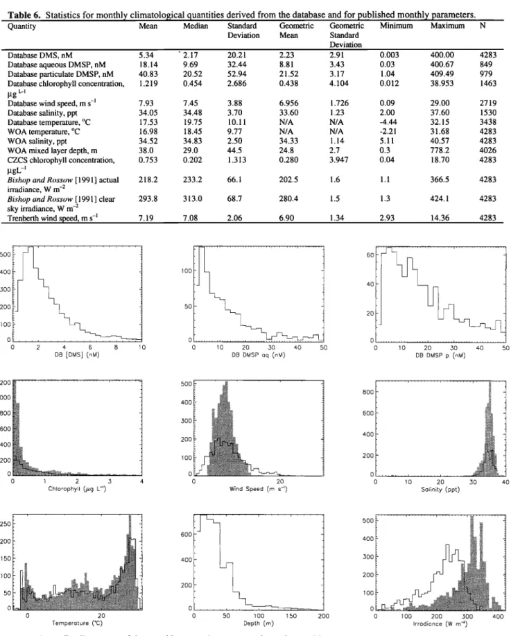
The statistical properties of the annual ocean data squares are
presented in Table 4 for the parameters that were contributed to
the database and for other published climatological parameters
in the DMS ocean data squares. The histogram distributions of
these parameters are shown in Figure 2. Both Figure 1 and Table 4 show that DMS varies over a wide range of values. The
distribution of DMS data is not Gaussian but is best fitted by a
lognormal distribution. Chlorophyll a concentration is skewed to
even smaller concentrations.
Efforts to find a correlation between the annual
Table 5. Correlation Matrix Between Database (DB) Parameters and Other Published Quantities Collected as Part of This
Study.
Parameter DB DMS WOA WOA WOA WOA
nitrate silicate phosphat oxygen
e
DB DMS, nM 1.000 - - -
(3317)
WOA nitrate, laM 0.2263 '1.000 - -
(3201) (3201) [99.99+]
WOA silicate, laM 0.2158 0.9379 1.000 -
(3207) (3201) (3207) [99.99+] [99.99+]
WOA phosphate, laM 0.3893 0.8148 0.7772 1.000
(3207) (3201) (3207) (3207) [99.99+] [99.99+] [99.99+]
WOA oxygen, mill 0.1962 0.6803 0.7158 0.6044
(3207) (3201) (3207) (3207) [99.99+] [99.99+] [99.99+] [99.99+] ETOPO5 Depth, m -0.2117 -0.1116 -0.1119 -0.1488 (3209) (3152) (3158) (3158) [99.99+] [99.99+] [99.99+] [99.99+] DB aq DMSP, nM 0.4380 -0913 -0.1596 -0.1726 (573) (539) (540) (540) [99.99+] [96.61] [99.98] [99.99] DB part DMSP, nM 0.4917 -0.0227 -0.0955 -0.0646 (659) (624) (625) (625) [99.99+] [42.65] [98.32] [89.34] DB chl, lag L '• 0.1939 0.0697 0.0568 0.0626 (1287) (1210) (1211) (1211) [99.99+] [98.46] [95.17] [97.11] DB wind speed, m s -• 0.0279 0.1145 0.1080 -0.0097 (2378) (2318) (2323) (2323) [82.78] [99.99+] [99.99+] [35.65] DB salinity, ppt -0.0073 -0.1876 -0.2395 -0.1882 (1375) (1320) (1324) (1324) [21.42] [99.99+] [99.99+] [99.99+] DB SST, øC -0.1727 -0.6918 -0.7012 -0.5957 (2900) (2831) (2837) (2837)
Depth DB aq DB part DB chl a DB wind DB
DMSP DMSP speed salinity DB SST 1.000 - (3207) -0.3748 1.000 - (3158) (3209) [99.99+] 0.0912 -0.3935 1.000 (540) (534) (573) [96.61] [99.99+] 0.1312 -0.2307 0.6159 (625) (621) (525) [99.90] [99.99+] [99.99+] 0.2077 -0.2922 0.1619 (1211) (1217) (489) 1.000 (659) [99.99+] [99.99+] [99.97] 0.1005 0.0124 0.0003 (2323) (2326) (410) [99.99+] [44.70] [99.99+] [98.35] -0.4720 0.3318 0.1118 0.1123 (1324) (1323) (406) (490) [99.99+] [99.99+] [97.61] [98.72] -0.9480 0.3148 -0.0515 -0.1091 (2837) (2832) (434) (513) 0.3826 (588) [99.99+] -0.1095 (478) 1.000 (1287) 0.0052 1.000 (843) (2378) [12.01] -0.1345 0.0833 (811) (1101) [99.99] [99.44] -0.1801 -0.2126 (997) (2295) 1.000 (1375) 0.1743 1.000 (1343) (2900) [99.99+] [99.99+] [99.99+] [99.99+] [99.99+1 [99.99+] [71.70] [98.68] [99.99+1 [99.99+1 [99.99+1
The numbers in parenthesis are the number of annual ocean data squares shared by each pair of quantities. The numbers in square brackets are the significance levels determined from Student's t test.
KETTLE ET AL.: SEA SURFACE DIMETHYLSULFIDE MEASUREMENTS 419
30 N. N:PST(E)
:':•CAL30 s ?iil
...
•:':'::::::::::::
..•,•,::,•;::•::•:•::•:ii'!•'•::'•'•'•'::'•;::•::'
•:::•::•
•:
:/::
::•:•::
•:;::::::':;':::::":::::'::::'•'::•':'•::::'
'•"::::::
•::•::;•:::::::
:::•:::•:
;•!'•:!
•!•::'::'
::?:::::::'::
'•'•'•:'"':':':"
'•:'":':::
'•'•'•
•::':'
:•:'
•:
•'::;'•:•:•:•:•:::•'•:•'•':'•
'•'•
'•':'""::'
'"'•'•'
:•;•:•:•::::::•:•:•:•;•::•i•i•:•.•::•:::•:::•:::•::•::;•:•:•::•i::
... ß
..•.•...i:i?
::•:
!::;i•:•:...:..:.ii::::ii•
...
•---
-- .. --
...
--•,..
•'?---..---,,,.•
....
.• .,,.
•...•.•--.,.,...
::::::::::::::::::::::::::::::::::::::::::::::::::::::
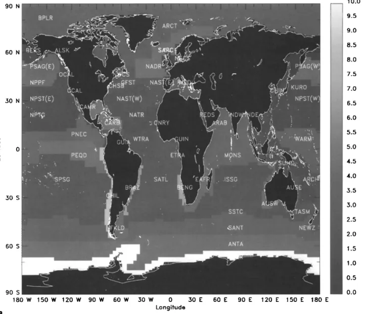
9O S 180 W 150 W 120 W 90 W 60 W 50 W 0 ,30 E 60 E 90 E 120 E 150 E 180 E LongifudeFigure 4. Unsmoothed
first-guess
field of annual
DMS sea
surface
concentration
(nM). The first-guess
field is
based
on average
sea surface
DMS concentrations
in the 57 global
biogeochemical
provinces
proposes
by
Longhurst et al. [1995].
1.5
1.0
0.5
0.0
climatological
DMS concentrations
in the database
and published
climatological
nutrient
values
were not successful.
Figure
3
shows
contour
diagrams
of the scatter
of points
between
DMS
and the other climatological
quantities
in the database.
Table 5
shows the correlation matrix between all the different pairs of
data sets together
with the number
of pixels and the percent
significance
of the calculated
regression
coefficient
against
a
zero-correlation
null hypothesis.
All the regression
coefficients
are small (but with very high significance
levels) and do not
indicate
a quantitative
relationship
between
DMS and other
parameters
that could be used as a predictor
for DMS
concentration in the world ocean. With respect to DMS
concentration,
the highest correlation was found with
climatological particulate
DMSP concentration,
but the
correlation coefficient was still only 0.49. The highest
correlation between the annual DMS climatology and a published
parameter
was 0.39 for phosphate
from
the World
Ocean
Atlas.
This was not high enough to serve as the basis of a first-guess
field for the sea surface distribution of DMS. Even if a
correlation had been found between the annual climatological
quantities, DMS is suspected to have a pronounced seasonal
cycle at high latitudes, and this information cannot be conveyed
in an annual average field of DMS concentration.
When the ocean data squares of annual climatological data
were sorted by the biogeochemical province according to
Longhurst et al. [1995], the correlations between the annual
parameters improved somewhat. The relationship between DMS
and the annual nutrient fields given in the World Ocean Atlas
was characterized by generally low correlation coefficients.
More biogeochemical provinces tended to have the highest
correlation between DMS and silicate rather than between DMS
and the other nutrients or dissolved oxygen. However, this
heightened
covariance
with silicate
was found in only 10 of the
40 biogeochemical
provinces
where there were more than 10
420 KETI'LE ET AL.: SEA SURFACE DIMETHYLSULFIDE MEASUREMENTS
,_'1 IOUaU
z