Application of Pontryagin's minium principle to filtering problems

MINIMUM PRINCIPLE TO FIL TERING PROBLEMS by

EDISON TACK-SHUEN TSE wtTA

SUBMIT TED IN PARTIAL FULFILLMENT OF THE REQUIREMENTS FOR THE DEGREE OF

MASTER OF SCIENCE at the

MASSACHUSETTS INSTITUTE OF TECHNOLOGY June 1967

Signature of Author

Deparh ment of Electrical Engineering, May, 1967 Certified

by----esis Supervisor Accept

APPLICATION OF PONTRYAGIN'S

MINIMUM PRINCIPLE TO FILTERING PROBLEMS by

EDISON TACK-SHUEN TSE

Submitted to the Department of Electrical Engineering in May, 1967 in partial fulfilment of the requirements for the degree of Master of Science.

ABSTRACT

The purpose of this thesis is to consider the formulation and solution of a class of linear and nonlinear stochastic problems pertaining to control and estimation. These stochastic problems are reformu-lated as essentially deterministic problems. The matrix minimum principle is used to derive necessary conditions for optimality; these are used to obtain optimal and suboptimal designs.

Thesis Supervisor: Michael Athans

I would like to express my sincere gratitude to Professor Michael Athans for his constant encouragement, friendly advice and sound criticism. The discussions with Professors Michael Athans, Fred

C. Schweppe, Donald L. Snyder and Mr. Patrick Lee are most

helpful and stimulating.

At this time I am happy to express my appreciation to Professor Lan Jen Chu for his encouragement, comment and support while acting as my Undergraduate Faculty Counselor. My interest in

stochastic processes relating to engineering problems comes from the inspiring teaching of Professor Wilbur B. Davenport, Jr. and

Professor Harry L. Van Trees, Jr.

I would like to also thank Mrs. Ionia Lewis for coordinating the thesis and Mrs. Clara Conover for typing it.

CONTENTS

CHAPTER I INTRODUCTION pag1

CHAPTER II CONDITIONS FOR OPTIMALITY 6

A. CLASS OF ADMISSIBLE CONTROLS 6

B. THE MATRIX MINIMUM PRINCIPLE:

A NECESSARY CONDITION FOR OPTIMALITY 8

C. A SUFFICIENT CONDITION FOR OPT IMALITY 14

D. DISCUSSION OF RESULTS 17

1. The Matrix Minimum Principle 17

2. The Sufficient Condition for Optimality 19

E. FUTURE RESEARCH 19

CHAPTER III NOISY STATE -REGULATOR PROBLEMS 20

A. STATE-REGULATOR PROBLEM WITH

DRIVING DISTURBANCE OF ZERO MEAN 21

1. Reformulation of the Problem 22

2. Application of the Matrix Minimum Principle 23

3. The Minimum Cost Functional 25

B. STATE-REGULATOR PROBLEMS WITH

DRIVING DISTURBANCE OF NONZERO MEAN 26

1. Reformulation of the Problem 27

2. Application of the Matrix Minimum Principle 28

3. Minimum Cost Functional 30

C. NOISY STATE-REGULATOR PROBLEM WITH OBSERVATION NOISE AND DRIVING

DISTURBANCE 32

1. Reformulation of Problem 33

2. Application of the Matrix Minimum Principle 37

3. The Minimum Cost Functional 41

D. DISCUSSION OF RESULTS 42

1. State -Regulator Problem with Driving

Disturbance of Zero-Mean 42

2. State-Regulator Problem with Driving

Disturbance of Nonzero Mean 43

3. State -Regulator Problem with Observation

Noise and Driving Disturbance 44

E. DISCUSSION OF OUR APPROACH 45

F

CONTENTS (Contd.) CHAPTER IV A. B. C. D. E. F. G. CHAPTER V

NONLINEAR STATE ESTIMATION WITH

QUADRATIC CRITERIA _page

FORMULATION OF THE CONTROL PROBLEM APPLICATION OF THE MINIMUM PRINCIPLE SEQUENTIAL ESTIMATION

APPROXIMATION OF THE OPTIMUM NONLINEAR ESTIMATOR

DISCUSSION OF RESULTS

DISCUSSION OF OUR APPROACH FURTHER RESEARCH

NONLINEAR ESTIMATION OF A FIRST ORDER QUADRATIC DRAG DYNAMICAL SYSTEM

A. STATE ESTIMATION OF A QUADRATIC DRAG

DYNAMICAL SYSTEM

B. APPROXIMATION OF OPTIMUM NONLINEAR FILTER: I

C. APPROXIMATION OF OPTIMUM NONLINEAR FILTER: II D. DISCUSSION OF RESULTS E. FURTHER RESEARCH CHAPTER VI CONCLUSIONS APPENDIX 1 APPENDIX 2 APPENDIX 3 APPENDIX 4 APPENDIX 5

MODEL OF CONTINUOUS WHITE NOISE LINEAR SYSTEMS DRIVEN BY

WHITE NOISE PROCESSES ESTIMATION OF GAUSSIAN WHITE NOISE PROCESSES INVARIANT IMBEDDING CALCULATIONS

A.5.1 MINIMUM FUNCTIONAL FOR

STATE-REGULATOR PROBLEM WITH DRIVING DISTURBANCE OF NONZERO MEAN

A.5.2 SOLUTIONS FOR THE SET OF 1\[ATRIX DIF-FERENTIAL EQUATIONS OF (t) and P (t)

CONTENTS (Contd.)

A.5.3 MINIMAL FUNCTIONAL FOR

STATE-REGULATOR PROBLEM WITH DRIVING

DIS-TURBANCE AND MEASUREMENT NOISE page 90

APPENDIX 6 GRADIENT MATRICES 94

APPENDIX 7 ASSUMPTIONS ON THE SYSTEM II 96

BIBLIOGRAPHY 98

1. State Regulator Problem with Driving Disturbance page 31 2. State-Regulator Problem in the Presence of

Disturbing and Observation Noise 35

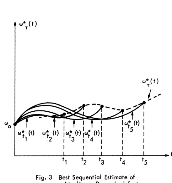
3. _{Best Sequential Estimate of a Nonlinear Dynamical System 55} 4. Approximation of Optimum Nonlinear Filter of a First

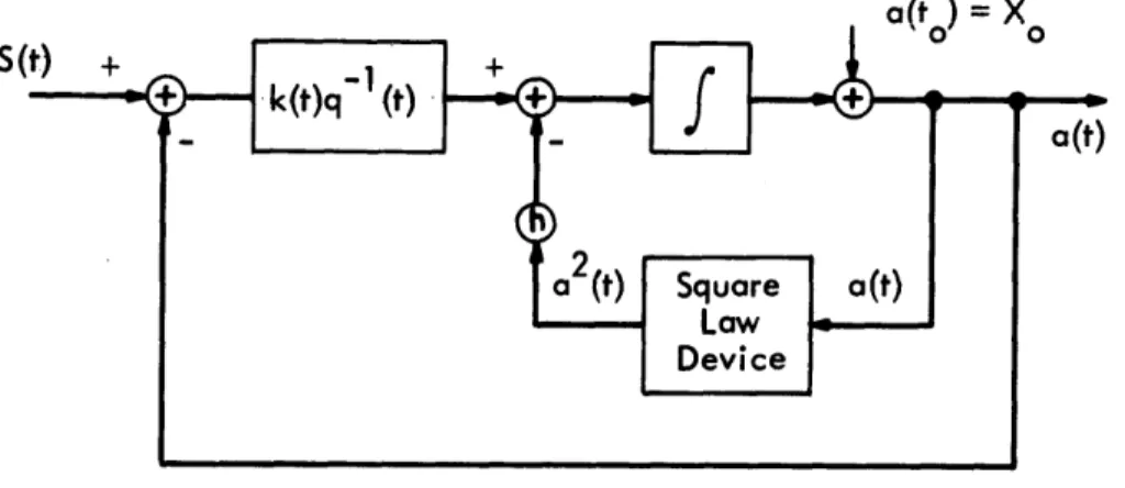
Order Quadratic Drag Dynamical System 67

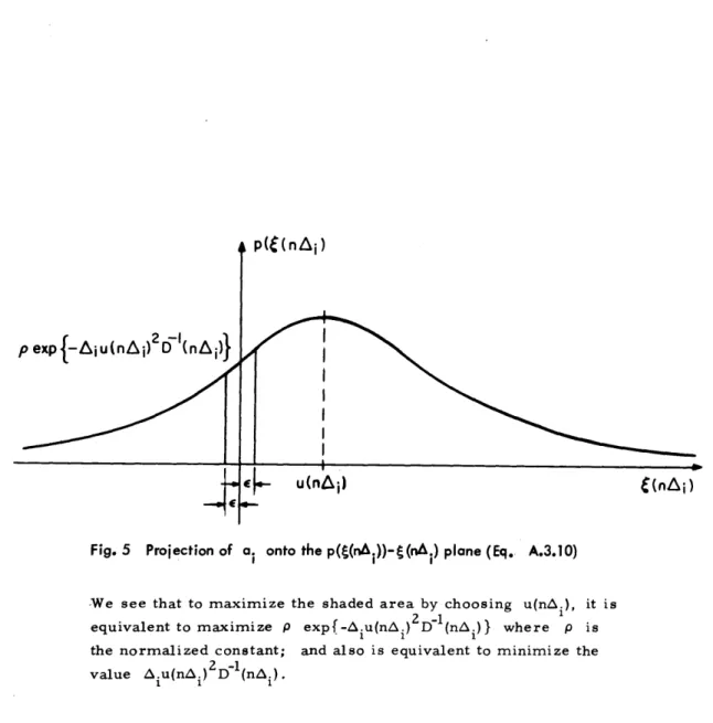
5. Projection of a onto the p(((nA.))-g(nA.) plane

Eq. (A.3.10) 80

NOTE TO THE READER:

Throughout this thesis, unless otherwise defined, lower case letters will stand for column vectors (e. g., x, y); upper case letters

will represent matrices (e.g., A, B); lower case letters with sub-scripts will denote components (e. g., xi will be the i-th component

1)1

of the vector x, a i will be the ij -th entry of the matrix A). The transpose of a matrix A is denoted by A'. The trans -pose of a column vector, x, is a row vector and is denoted by x'.

Let A be an nxn square matrix; the trace of A is defined as

n

Tr A = a..

Let H(x , x1 2' ' 'xnm) be a scalar function; we shall de-note it by H(X). The gradient matrix is defined by

alH(X) al8 (xl , x12' ' ''nm

8X

ax..

1)

Let Q be a metric space, the closure of Q will be denoted by 0.

Let V be an inner product space, if vi, v2 are in V, the

inner product of these two elements will be denoted by < v, v2 V M _nm will denote the set of all nXm matrices.

R will denote the product space of ordered n-tuples of real n

INTRODUCTION

The general problem of engineering system design in the presence of uncertainty has received much attention. (See for example Refs. 12, 28.) It turns out that design problems can be formulated and viewed as special cases of general decision problems under uncertainty. 2 8*

Inthis thesis we shall approach these engineering problems fromthis point of view.

In a general decision problem, there are basically three nonempty sets: D, the action space; N, the states of uncertainty, and a well

-ordered set 0, the set of outcomes; furthermore, there is a mapping M

M : DXN-O (1.1)

Loosely speaking, we are given the three sets, D, N and 0, and the mapping M, and we are to find an element in D, such that, under all uncertainties, it will be in some sense more preferable than the other elements in D.t Unfortunately, few specific results canbe obtained under this general formulation. If we attach more structure to the sets N, D and 0, and also be more specific about the mapping M, then we may be able to findthe "best" action amongthe elements of the action space D.

Let us consider two special cases that are of interest. In the first case, let us suppose that N consists of only one element, D is a set of measurable functions defined in the time interval [t, t ],

o

is a set of 3 -tuples (x, y, y0) where x and y are measurable functions defined in the time interval [t t ] and y is a real number. The mapping M maps x into (x, y, y0) where x, y and yo are related by

Superscripts refer to numbered items in the Bibliography.

tFor more details see Ref. 28.

-1-

-2-y(t)

= fM(x, y, t)

(1.2)

y(t)

_{- y}

J

The elements in 0 are well-ordered, i.e., there is a functional from 0 into the set of real numbers R

J : 0 -- R (1.3)

such thatt

(x, y, y_) > M ,, 70) iff J(x, y, y) < fly, ) (1.4)

We immediately recognize this as a deterministic optimal control problem where we choose x to minimize J(x, y, y0) subject to the constraint (1.2). For this class of problem, the Pontryagin maximum (or minimum) principle gives the necessary conditions for optimality. (See Refs.1, 23 and 25) Another case is when D = N = set of

measurable functions defined in the interval [ t , t], 0 is a set of 4 -tuple s (x, n, y, y0) where x, n, y are measurable function and y0 is

a re al numbe r; the mapping M maps (x, n)c D X N into (x, n, y, y 0)

where x, n, y, yO satisfy

y

t) = fM(x, n, y, t)

(1.5)

y(t

)

=

y

The set 0 is well-ordered, and

(x, n, y, yO) > (x, , y, 70) if f J(x, n, y, y0 , , , y0) (1. 6)

where J is again a functional which maps 0 into the set of real

tThe ordering in 0 is defined in such a way that if o 1 in 0 is more preferable than o2 in 0, then o₁ > o2 '

numbers R. This class of problems we shall call optimal control problems under uncertainty. In this case, it is difficult to say which decision is more preferable, because it depends on the uncertainty which is unknown to us. If we suppose further that the uncertainty

space N has a if-algebra structure21 and 11 and defined on it a proba-bility measure, then it is reasonable to say that the decision x i s

more preferable than x if

f

J(x,

n, y, yO)d

<

fJ(3r, iT, 7, 7)d

(1.7)

N N

where i is the measure defined on the a -algebra of N. This type of problem is refered to as a stochastic control problem. 13, 14, 30 The mathematical technique for solving this specific formulation of problem is rather involved because we are dealing with stochastic differential equations, and stochastic integrals instead of ordinary differential equations and integrals. 20,29,31 Yet, if we note that the stochastic control problem is but one special formulation of

un-certainty problems, we can reformulate the problem to avoid the dif-ficulties that may arise in stochastic problems. This thesis represents an attempt in this direction. We shall reformulate the problems as deterministic control problems, and the nature of uncertainty may be incorporated in the functional J or in the reformulation of the prob-lem; in this manner we will be able to apply the Pontryagin maxi-mum principle.

Pontryagin et al.23 proved the maximum principle which is ap-plicable to the minimization of a given functional subject to

dif-ferential equation constraints. In Chapter II, we shall extend it so as it becomes applicable when the system is described by matrix dif-ferential equations. We shall refer to the result as the

matrix-minimum principle.

In Chapter III, we shall investigate stochastic regulator problems. These problems had been investigated by Florentin13 and Wonham. 30

-4-Their approach is to define a stochastic control problem and apply the technique of Dynamic Programming to obtain the optimal control.

This further reduces to the problem of solving a partial differential equation.13 Specific results can be obtained if the system is linear with quadratic criteria.13

We shall deviate from this conventional approach. First, we shall reformulate the stochastic problem as a deterministic problem; then, we shall apply the matrix minimum principle to obtain the optimal control. We shall see that the nature of uncertainty will be incorporated in the reformulation of the problem. The results ob-tained are found to be the same as those obob-tained by the Dynamic Programming approach. In this framework, we can easily solve the optimal regulator problem when observation noise is added to the output of the system. This problem has also been studied by Meier, 22 Roberts, 24 and Wonham30 using a different approach from our own. We shall also find that the results obtained in the course of this

re-search work agrees with theirs.

In Chapter IV, we shall study the nonlinear filtering problem. This problem has been investigated by Bucy, 8 Cox, 9 Kushner, 9, 20 Snyder, 27 and Wonham.31 The approach of these authors is the

stochastic one. Few results of practical significance have been ob-tained; 9 this is due to the difficulties that arise in most stochastic processes. Other approaches have also been attempted.7, 10

In this thesis, we shall use the decision approach; we shall formulate the problem as a deterministic control problem while the nature of uncertainty is incorporated in the cost functional. A justification for this formulation will be given. If the system is not very nonlinear, we shall see that the results obtained here agree with the results obtained by Snyder. 2 7

In Chapter V, we shall work on a simple example on nonlinear filtering. We shall take a quadratic drag system and investigate the effect of the second order dynamic of the nonlinear system. This

example also shows some of the advantages of the decision approach over the conventional stochastic approach.

In summary, the work is an attempt to study a new viewpoint toward design problems. Instead of worrying about the existing problems in stochastic processes, we shall concentrate on the physi-cal behavior of the system under uncertainty. Extensions may be possible when the space of uncertainty does not have a e--algebra structure. Also it is hoped that this study will provide more in-sight into the structure of the system to be designed.

CHAPTER II

CONDITIONS FOR OPTIMALITY

We shall be considering the mathematical problem of mini-mizing a given functional subject to a given matrix-differential equations. We can view this as an extension of the work by Pontryagin, et al.23 because the nature of the proof depends heavily on their results. To formulate the problem vigorously, we shall state in a general context the definition of class of admis-sible control, even though the set of admisadmis-sible controls we shall be considering is a particular class. We shall then state and prove the matrix minimum principle, which gives us a necessary condition for optimality. The local sufficient conditions will be stated and proved. The result of this work is, in fact, "buried" in Pontryagin's work, but because of the mathematical form of the results obtained we may view Pontryagin's minimum (or

maximum) principle as a special case of the results obtained here.

A. CLASS OF ADMISSIBLE CONTROLS

In this section we shall define mathematically the class of functions that we are allowed to choose in our optimization problem. Physically, the class of functions that we are considering has the property of separating past and future.

Let 0 be an arbitrary subset of the r-dimensional vector space E . We shall call the set Q the control region. Let u be an element in 0 ; u is represented by the r-tuple (u . .. , r'u

Consider a function u(t) defined on the time interval { t , tI]

with range in Q ; we shall call u(t) a control. The control u(t), t

<

t

< t ,

is measurable if the set T = {t

<

t < t 1 :u(t)c U} is

0- - 1' U

-measurable for every open set UCEr (see Ref. 21). The control u(t), t < t < ti, is bounded if the set of points u(t), t < t

<

t

o- - o - 1

-has a compact closure in E r. We shall now give a precise defini-tion for the class of admissible controls.

Definition 2. 1: Let D be a subset of the set of all [t, ,t]

controls defined on the interval [ t , t 1 ] . D[ t0 , t ] is called a class of admissible controls if for any u(t), t < t < t, in D[ t. t we have

(1) u(t), t < t < ti, is measurable and bounded. (2) For vE Q , the control defined by

for t'<t

<t"

(2.3) v

u(t)

for t < t

<

t' or t"

<

t

<

t o- - - 1

is also in D[ tO, t

t'

(3) For a > 0, the control defined by u"(t) = u(t-a); t + a

<

t

<

t + a o -- 1 (2.4)

is also in D [t t

1

'

(4) u(t), t' < t < t", is in D where - -' [t',t"] t < t'< t"< t .

The class of all measurable and bounded controls. and the class of all piecewise constant controls are examples of class of admissible controls. In this chapter, we consider the case where Er = Rr'

and D tO, t is the set of all bounded piecewise continuous function u(t), t

<t <t,

such that

-8-( 1) UMt C Q t o< t

<

t (2. 5)

(2) u(t -) = u(t) t

<

t

<

t (2.6)

B. THE MATRIX MINIMUM PRINCIPLE: A NECESSARY CONDITION FOR OPTIMALITY

Consider the system of differential equations dx..

dt = fij (xi x _{1 2} ' ' ' . nmlu1Ul , 2, . .ur ) i=1 ... n (2.7)

or in the matrix form dX ₌

F(X, U) (2.8)

3f..

The functions f .(X, U) and a are assumed to be given

mn

and to be continuous on the direct product R X?7. Consider the nm integral functional tI J = f '(X, U) dt ; t ₁ Free (2. 9) t 0

We wish to choose among all admissible controls those which will transfer X(t) from X(t ) = X0 to X(t1 ) = Xi, and which will give us a minimum for the functional (2.9). The desired controls are called optimal controls. We now state and prove a necessary con-dition for optimality.

Theorem 2. 1: (Matrix minimum principle) Let U'(t) be an admissible control with range Q, which transfers (X t ) to S = {X1}X(T',T2). Let X '(t) be the trajectory of (2.7) corre-sponding to U'(t) with X',(t0 ) = X,X'(t )= X. In order that

U*(t)

is optimal, it is necessary that there exist a scalar and a nxm costate matrix P*(t) such that

(1) X*(t), P*(t) satisfies the canonical equations:

p I> 0 0-X*(t) _8P(t) 8H * P*(t) (2. 10) a- (t) * Satisfying the boundary conditions

X*,(0t

= X9 , X*(t ) X with H!= p f (X, U) + 00o (2. 11) (2. 12) Tr[F P'] (2) _{H(X*(t), P*(t), U, pO)} function of U over 0 H(X*I(t), P*(t), U*(t),

has an absolute minimum as a at U = U'(t), t <t<t _0- , i.e.,

-- 1'

p) = min H(X*(t), P*(t), UEQ

U*(t), p*) ₀ = 0 t _o0-

<

t

<

_- t₁ Proof: _{Consider a mapping <-:Mnm -+Rnm}

x11 x l x 2 1 x - nm defined by (2.15) U, p*) 0 (2. 13) (2. 14) (3) HX () *t,

-10-Clearly the mapping a- is one-to-one and onto the whole space R . We shall consider U(t) as a point in QCRrs where u .(t)

is the ijth component. With these transformation, we have con-verted the original problem into an equivalent new problem: given

dy. (t)

dt i l '' nmUt u i=1, .. ., nm (2.16)

wher g1 Ay A -f11

where g f 1, g2 f12' ' m+i f 21' ' nm nm (2. 17)

a g.

g (y(t), U(t)) and --:L are given and continuous

t1

J

=

f

9(y(t),

U(t)) dt

(2. 18)

t

0

-where go(y(t), U(t)) = f (X(t), U(t)) (2. 19)

We are to find an admissible control U(t) CQ , which will transfer y(t) from y(t ) = y = a-(X ) to y1 = a-(Xl) such that the functional (2.18) will be minimized. For this equivalent problem, Pontryagin has proved the minimum (or maximum) principle which gives the necessary condition for optimality: in order that U* (t) for the above special case to be optimal, it is necessary that there exists a

scalar p' > 0 and a costate vector q*(.t) such that (see Ref. 1) 0-8H Y 0 (1) y

~

..*(t) = -q t (2.20) 3H0 M~t a 8yMt

with boundary conditions y*(t)= y ; y*(t ) = y,

A

where H 0= _{pg(y(t), U(t)) + <g, q> R} nm

(2) H (y'(t), q*(t), U*(t), p

)

= min H (y''(t), q''(t), U, p

UCe 0

H0 (y(t), q(t),U*(t), p0) = 0 Since a- is one to one onto, a-~ exi from R to M where a- o o-(X) = X.

'LII 1

sts and it is a mapping Let us define

P(t) = a- (q(t)) (2.25)

H(X(t), P(t), U(t), p0) = _{H0 (-(X(t)), o-(P(t)), U(t), po)}

= H (y(t), q(t), U(t), pO) (2.26)

Let U '(t) be the optimal control for the original problem; then it is also optimal for the equivalent problem; since p" > 0

exist, this implies that p* > 0 and P*(t) exist.

and q*(t) The q*(t) satisfies (2.20), (2.21) and (2.22); we shall show that this implies P*(t) satisfies (2.10), obtain (2.11) and (2.12). We rewrite (2.20) to 3H 1 1 (t) 8q M M 0 = Im(t) 3 -m

irm(t)=*

(t) = -api ₁ &-H ap1m 0 )q nm (3) (2.21) (2.22) (2.23) (2. 24) 111 y*(t) (2.27) 8H

-12-We have a similar set of equations relating _{p (t)} 13

and thus we see that (2.20) yields the set of the matrix equations:

X*t = aH

aP(t)

H

P*(t = OH

pit M -X(t)

J

Equation 2. 21 implies that

0 = - (y ) = X ; X*(t ) = X

Equations 2.22 and 2.26 imply that

H(X(t), P(t), nm U t), Po) = p0g0(y, U) + X n, m = Pof_{0 (X, U) +}

i1,

j

= p0f0 (X, U) + Tr [ FP']

Also by (2.25), (2.26), we see that (2.23), (2.24) can be written as (2.13) and (2.14) respectively.

Q.E. D.

For the case where the target set S = S X , T2)' S1 CMm' we can establish the transversality conditions: the matrix P*(t) is transversal (normal) to S at X*(t₁), i.e.,

= Tr [X*(t₁ ) P*'(t)] = 0 with - H lj (2.28) (2.29) f.. p.. (2.30) gi qi

<

a-(*(t, a-(X*(t ))>

We shall now state without prooff the results of two control problems which we shall use in Chapters 3 and 4.

Control Problem 1:

Given X(t) = F(X, U) (2.31)

and the cost functional

t

J = K(X(t ₁)) + f (X, U) dt

where K(X(t ) is a scalar function. transfers X(t) from X(t ) = X to fied and the cost functional (2.32) is

We are to choose X(t 1) such that (2 minimized.

U(t)cQ which .31) is

satis-Theorem 2.2: In order that U*(t) be optimal for the control problem 1, it is necessary that there exist a nonnegative constant p* and a costate matrix function P*(t), such that (2.10), (2. 11), (2. 12), (2. 13) and (2. 14) are satisfied. In addition we must have

8K(X(t ₁₎₎ P''(t_{1) = 8X(t)} ( X''(t ) Control Problem 2: Given X (t) = F(X, U) (2.34) J = K(X(t )) + f (X U) dt

For a proof in the vector case, see Ref. 1.

(2.32)

(2.35)

-14-We are to choose U(t)cQ which transfer X(t) from X(t ) to X(t 1) such that (2. 34) is satisfied and the cost functional (2. 35)

is minimized.

Theorem 2.3: In order that U*(t) be optimal for the control problem 2, it is necessary that there exist a nonnegative constant p and a costate matrix function P*(t), such that (2. 10), (2. 11), (2. 12), (2. 13) and (2. 14) are satisfied, in addition we must have

P*(t 8K(X(t))

P ) - 8X(t (2.36)

X*(t0)

C. A SUFFICIENT CONDITION FOR OPTIMALITY

We shall now establish a sufficient condition for local opti-mality under a stronger assumption on the cost functional.

Consider the control problem:

X (t) = F(X, U, t) (2.37)

with cost functional

tl

J(X , U, t)

=

f

(X(t), U(t), t) dt

(2.38)

t 0

We wish to choose among all admissible controls with range in Q the one which transfers X(t) = X to X(t 1) = X e S such that the functional (2.38) is minimized. It is shown in (2.38) explicitly that the functional depends on the initial states X0, the initial time t and the particular control chosen.

0 A

Let U(t), t < t < t , be a particular control which transfers

(X , t ) to S = S1

X(T,

T2); we shall denote the corresponding trajectory by X(t). We shall write

tI

A A f A A

J[X(t), t, U] = f(X(T), U(T), T) dT (2.39) t

A

Since for every control U(t), to<< t < t there corresponds an unique trajectory X(t), t0 << t < t, we can write the functional (2.39) as a function of the states and time only, i.e., we can uniquely define

A[At) 1, [ A A

J[ Xt), t]

J[

X(t), t, U]

; t_

< t

<

t

(2.40)

A A

We shall assume that J[ X(t),t] is a continuously differentiable function with respect to its arguments on a region ACM X(T 1, T2)

A n

with (X(t), t)cA ; t

<

t

<

t .

Before proving the sufficient condition for optimality, we need some definitions to simplify the statements of the theorem.

Definition 2.2: Let H(X, P, U p , t) be the Hamiltonian

H(X, P, U, p 0t) = p0 f (X, U, t) + Tr [ F P'] (2.41)

If for each point (X, t) in A, the function H(X, P, W, p , t) has a unique absolute minimum with respect to all WcQ at W = U(X, P, t), then we say that H is normal relative to A or that our control problem is normal relative to A, and U(X, P, t) is the H-minimal control relative to A.

Definition 2.3: If H is normal relative to A and if U (X, P, t) is the H-minimal control relative to A, we shall call the partial differential equation

+ H [ X, (, t), (X (X, t), t] = 0 (2.42) with boundary condition

J(X,t) = 0 for (X,t)c S (2.43)

-16-We shall state and prove the sufficient condition for local optimality. The technique of the proof is similar to that used in proving Theorem 2. 1; for this reason, we shall outline the argu-ment instead of giving the rigorous formal steps.

Theorem 2.4: Suppose that A = A X (,T ₂) ; A IC M and that H is normal relative to A such that U(X, P, t) is the

A

H-minimal control relative to A. Let U(t) be an admissible con-trol such that:

A

(1) U transfers (X ,t

)

to S

A A

(2) _{If X(t) is the trajectory corresponding to U(t),}

then A

A

(X(t), t)c A t _0-

<

t

<

t (2.44)

- 1

A

(3) There is a solution J(X, t) of the H-J equation (2.42) satisfying the boundary condition (2.43), such that

A

U(t) = U(X(t), (X(t), t), t] (2.45)

A

Then U is an optimal control relative to the set of controls U that generate trajectories lying entirely in A, and

J[X(t),t,0

=

J[X(t), t]

t

<

t

<

t

(2.46)

Proof: Let A = o-(A ) X (T, T2), where a- is the same map-ping defined by (2.15). _1, Let H be defined as in (2.26). If H is

0

normal relative to A, then H is normal relative to A . Through the mapping a-, we can rephrase our assumptions: we have that H is normal relative to A and that U(y, q, t) is the H-minimal control relative to A . _{U(y, q, t) is an admissible control such}

that

A

IfAt A

(2) If y(t) is the trajectory corresponding to U(t), then

(y (t) , t) E A t o< t < t (2. 47)

0 0- - 1

(3) There is a solution J(y,t) of the H-J equation (2.42) satisfying the boundary condition (2.43) such that

A

$(t)

=

U

y(t), 8JAt), t), t] (2.48)

By

where y = -(X) ; q = c(P) ; y0 = o-(X ) (2.49)

A

Then we know (see Ref. 1) that U is an optimal control relative to the set of controls U that generate trajectories lying in A and

0

J{ (t), t, U] = J[ yt) t] t

<

(2 .50)

A

This implies that U is an optimal control relative to the set of controls U that generate trajectories lying in A and

J[ X(t), t,

$]

= J{X(t), t] t 0< t

<

t (2. 51)

o-- 1 (.1

Q. E. D.

If the region A is Mnm (T1, T2), then the theorem will give a global sufficient condition for optimality.

D. DISCUSSION OF RESULTS 1. The Matrix Minimum Principle:

From the nature of the proof, we see that its validity hinges on the construction of an one-to-one onto mapping a- from the space Mnm to R nm. If we examine the mapping a- carefully, we see that it is a linear mapping. If we define an inner product in the space Mnm by6

<X, Y> = Tr[XY'] (2.52)

-18-then we see that the mapping a- also preserves the inner product because we have

<o-(X), T(Y)>R =

x ijyij

= Tr[XY'] nm

= <X, Y>M (2.53)

nm

This implies that the mapping a- preserves the metric distance be-tween elements in M . Thus the spaces M and R are

nm nm nm

algebraically and topologically equivalent. By comparing (2. 8) and (2. 16) we see that the differential structure of M can be viewed through that of R . Abstractly, the two spaces, M and

nm nm

R nm have the same differential, algebraical and topological structures; thus the results that hold in one space must also hold in the other space and vice-versa. Notice that the statements of the matrix minimum principle are just expressing the Pontryagin's principle in terms of the elements and operations on the space Mnm

The proof of the matrix minimum principle relies heavily on the fact that the mapping - is nonsingular, as this guarantees the existence of P*(t) from (2.25). Let us consider the case

where we required that the state matrix X is a symmetric matrix. Then, if we consider the range space of - (acting on the set of all nxn symmetric matrices), then the range space will be a proper subspace of R . Therefore, the existence of q*(t) in

nn

-R does not guarantee the existence of - (q~(t)) in the original nn

space for now the inverse mapping is not defined on the entire space Rnn, and q*(t) may not belong to the range space. Simi-larly the proof breaks down if we assume any functional relations between the entries of the matrix X. This means that we must view the space Mnm as a nm-dimensional vector space. This point is very important, since it tells us when the matrix minimum principle is applicable.

The matrix minimum principle gives a set of necessary con-ditions that an optimal control must satisfy. Usually we first find all the controls that will satisfy the necessary conditions; these controls are called extremal controls. Among these we are to find the one that is optimal. The general questions as to the existence and uniqueness of the optimal controls is still an open area of research.

2. The Sufficient Condition for Optimality

Theorem 2.4 is a local sufficiency condition. In the proof we specified the region A a priori; yet, in practice, we are to find a suitable region A in which the theorem may be applied.

Note that the H-J equation is a partial differential equation with given boundary conditions; in general, there are difficulties in solving this partial differential equation. For this reason, we shall mostly use the H-J equation as a check on the optimality of the extremal solutions obtained by the use of the matrix mini-mum principle.

We note that the constant p* which appears in Theorem 2. 1 0

is constrained to be nonnegative. In most cases which are of interest to us, p* will be positive; (Ref. 1) for this reason, in the subsequent chapters we shall set p =1.

0

E. FUTURE RESEARCH

From this approach, we see clearly that the validity of the minimum principle relies on the algebraical, topological and

dif-ferential structures of the state space we are interested in. It seems (to the author) that the results may be able to extend to the case where the state space we are considering is an infinite (but countable) dimensional Hibert Space, on which a differential struc-ture is defined.

CHAPTER III

NOISY STATE -REGULATOR PROBLEMS

In this chapter and the next, we shall apply the matrix minimum principle to two general types of problems of engineering importance. Suppose that we wish to regulate (i.e., bring near zero) the states of a linear dynamical system. We shall investigate the two cases:

1. systems with driving disturbance only

2. systems with driving disturbance and measurement noise

These problems had been studied using the Dynamic Programming 13 30

approach. ' _{Specific results for linear system with quadratic}

13 30

criteria had been obtained. ' In this chapter, we shall approach the same problem from a different viewpoint. The results obtained in this work agree with the existing results; it will be seen that the new approach sheds more light on the structure of the system, and that it will be useful in the design of a suboptimal control system

subject to some constraints imposed by the designer.

We shall now outline the general idea of our approach to these problems. By a reasonable argument, we make an assumption about the form of the optimal control with some undetermined parameters.

The optimal control is completely specified if we set the parameters at their optimal values.

If the disturbances are modelled as white Gaussian noise, (see Appendix 1) then the states of the system turn out to be Gaussian; thus, one can completely describe the vector processes by their second and first moments. From the given system and the known statistics of the disturbance, we can write the dynamics of the second and first moments of the vector processes. The moments of the vector processes are regarded as the states of a new dynamical system. In so doing we have converted a stochastic problem into a deterministic problem so that the matrix minimum principle de

-rived in Chapter II can be applied. We shall use the Hamilton-Jacobi

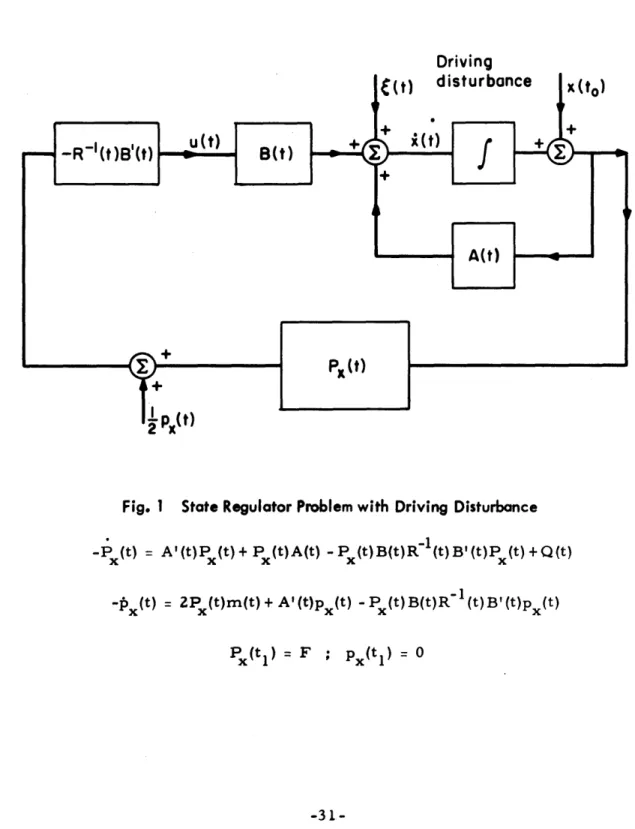
-20-Consider the plant k(t) = A(t) x(t) + B(t) u(t) + (t) x(t) A(t) u(t) B(t) (t)

(3.1)

is an n-vector is an nxn matrix is an r -vector is an nXr matrix

is an n-vector white Gaussian Process We assume that we

shall assume that

know the statistics of

a(t).

For simplicity we

E [ ((t)] = 0 ; E[ (t)('(T)] = D(t)5(t -T)

and that

to

_<

_t

_<

_t

We want to find u(t), t

<

t < tI, which will regulate the states to zero when x(t0) = x

/

0, with some constraints on the energy of the control function used. We choose a cost functional which will indi-cate the performance of the system, and also gives a simple form for the optimal control. A reasonable choice of the cost functional is

tI J = E[ <x(t1), Fx(t1)>+f <x(t), Q(t) x(t) >+ <u(t), R(t) u(t)>dt] t 0

(3 .4)

where

(3.2)

(3.3)

equation to check the solution obtained by the application of the mini-mum principle. The minimum value of the cost functional shall be derived so as to analytically describe the performance of the system.

A. STATE -REGULATOR PROBLEM WITH

DRIVING DISTURBANCE OF ZERO MEAN

-22-where F and Q(t) are nxn positive semidefinite matrices, and R(t) is an rxr positive definite matrix.

1. Reformulation of the Problem:

We shall now fix the structural form of the optimal control. We assume here that there is no observation noise; thus, we assume that we know the exact states of the system at any instant of time.

The states at any instant of time are what we need for describing completely the future behavior of the system with different control functions applied. The optimal control must be a function of maxi-mal information. Thus we see that the optimal control at time t must be a function of the states at time t and of the time t, i.e.

u(t) = g(x(t), t) (3.5)

When the variance of the driving disturbance (t) approaches zero, this means that

a(t)

becomes more and more deterministic and approaches its mean which is equal to zero. For this limiting case, we know that the optimal control is generated via a linear feedback law, i.e.,

u(t) = M(t) x(t) (3.6)

Since the effect of the disturbance (t'), t < t'

<

t, is included in the state at time t, x(t), it is reasonable to argue that the presence of disturbing noise should not change the form of the optimal control. For this reason, we fix the structural form of the optimal control to be a linear time -varying feedback law. In other words, we as

-sume that the control is generated from the state by

u(t) = M(t) x(t) (3.7)

where M(t) is an rXn matrix with, as yet, undetermined entries.

Substituting (3. 7) into (3. 1), we have

k(t) = [ A(t) + B(t) M(t)] x(t) + (t) (3. 8) From (3.8) and the statistics of the noise (3.2), (3.3), we can write the dynamics of the second moment of x(t). (see Appendix 2)

Z (t)= [ A(t) + B(t) M(t)] (t) + F (t)[ A'(t) + M'(t)B'(t)] + D(t) (3.9)

where Z (t) = E[x(t)x'(t)] (3. 10)

The cost functional (3.4) can now be written as t1

J

=

T r[ F E (t

1

)] +f

Tr[Q(t)z

E(t) + M'(t) R(t) M(t) Z (t)] dt

(3. 11)

t 0

The new optimization problem we have to solve is: Given the matrix differential equation (3.9) and the cost functional (3.11) choose M(t) (which is unconstrained) so that the functional (3. 11) is minimized subject to the matrix differential equation (3. 9).

2. Application of the Matrix Minimum Principle

We have changed a physical problem into a mathematical problem for which the results obtained in Chapter II can be applied directly. We shall now apply the matrix minimum principle to derive an extremal matrix M(t) which is now viewed as the control function for the new system (3. 9). Toward this end, we form the Hamiltonian, in which P (t) is the costate matrix associated with Z (t),

H = Tr[ (A(t) + B(t)M(t)) P (t) + _{x xx}(t)(A'(t)+ M'(t)B'(t))P' (t)_X

(3.12)

-24-The necessary condition that Z (t), P'(t) satisfy the canonical equations yields:

(t)= A (t) + B+ (t)[ A'(t) + M* '(t)B'(t)] + D(t) (3.13)

x x x

S(t) [ A'(t) + M*(t) BI(t)] P (t) + P (t)[ A(t) + B(t)M*(t)]

+Q(t) + M* (t) R(t) M*(t) (3.14)

The transversity condition yieldst

3Tr[FE (t

]

P (t ) 1 = F (3.15)

xax

1

A necessary condition for M*(t) to minimize the Hamiltonian is given by

* *

8H(Z*(t), P*(t), M(t))

8Mx * 0 (3 .16)

8M(t) _{M(t)=M (t)}

Differentiating (3.12) with respect to M(t) and setting it to zero, -1*

we have M (t) = -R (t) B'(t) P (t) (3. 17) x

By the assumption that R(t) is positive definite, then indeed Eq. 3. 16 gives us the M (t) which minimizes the Hamiltonian. Substituting (3.17) into (3. 14), we have the complete solution which satisfies the necessary conditions for optimality:

-* * -l *

-P (t) - A'(t) P (t) + P (t) A(t) - P (t)B(t)R (t)B'(t)P (t) + Q(t) (3. 18) with boundary condition

P (tl) = F (3.19)

The feedback gain is given by

M (t) = -R (t) B(t) P (t) (3.20) where P (t) satisfies (3. 18) and (3. 19). We note that Eq. 3. 18 is the familiar matrix Riccati differential equation.

3. The Minimum Cost Functional We shall now show that

E[ J(x(t), t)] $J*[ Z (t), t] = Tr[ P (t)(t)] + f(t) (3 .21) where

_f

(t) = _{-Tr[ D(t)P (t)]}

(3.22)

f(t 1) = 0

will satisfy the H-J equation with M(t) = -R~ (t)B(t)P (t) and P (t) satisfies (3. 18) and (3. 19). Thus the solution obtained by the appli-cation of the matrix minimum principle satisfies the sufficient con-ditions and, therefore, is optimal.. Clearly, the boundary condition is satisfied, because

J* [x (t

),

t]

= Tr[ P (t

)

(t

)]

Tr[FE (t

)]

(3.23)

Also we have a J* E (t), t] _df

8

t = T r P (t) Z (t)] + df (3.24) 8J* FE (t) , t] 8a E(t) P x(t) (3.25) x

By (3. 24), (3.25), (3.22) and the relation M(t) = -R ~(t)B'(t)P (t) where P x(t) satisfies (3. 18) and (3. 19), we see that direct substi-tution yields

A

-26-* [ ) *

= 0 (3.26)

This shows that the cost functional defined by (3. 21) and (3.22) is the minimum cost functional which describes the performance of the

optimal system and that the optional control law is described by (3.20), (3.18) and (3.19).

B. STATE-REGULATOR PROBLEMS WITH

DRIVING DISTURBANCE OF NONZERO MEAN

We now consider the plant (3. 1) with a driving disturbance which has a nonzero mean, i. e., we assume

E [ (t)

i

=

m(t)

(3.27) Let us define (3.28) 0 (t) = g(t) - m(t) We assume that E[ ( (t) -m(t))((t) -m(t))'] =_ E [ 0(t) ' (t)] - D(t)5(t -- ) (3.29) Thus we can write (3.1) as

k(t) = A(t)x(t) + B(t)u(t) + m(t) + (t) (3 .30) where m(t) is now a deterministic quantity, and the statistics of

o (t) are

E[ 0(t)]

=

0

; E[g 0(t)(' (t)] = D(t)S(t-T)

The problem is to choose u(t) such that the functional

J

= E[ <x(t

1

), Fx(t

1

)> +

f

is minimized subject to (3.30).

(3.31)

(3.32)

We see that mean of the disturbing noise effects the states of the system in a deterministic way; we would expect that the form of the optimal control must contain a part which is independent of the

ob-served states, but only dependent on the structure of the system and the statistics of the disturbance.

1. Reformulation of the Problem Let us decompose the state into

x(t) = xr (t) + xd(t) (3.33)

and the control u(t) into

u(t) = ur(t) + ud(t) (3. 34)

where x r (t), x ur(t), ud\t) satisfy

r (t) = A(t)xr(t) + B(t)ur(t) + o(t)

(3.35)

xd(t) = A(t)x d(t) + B(t)ud(t) + m(t) (3.36)

By comparing (3. 35) with (3. 1), (3.31) with (3. 2), (3.3), we can use the same argument to fix the form of the optimal control ur(t) as a linear feedback; Eq. 3.36 gives the form of the optimal control ud(t) which is a linear feedback plus a function (predetermined) of time. _{Since the structure of systems (3.35) and (3.36) are the same,} the feedback gain for each case is the same.i Thus we can write

u(t) = K(t) x r(t) + K(t)xd(t) + k(t) = K(t)x (t) + k(t) (3.37)

-28-The term k(t) is necessary to cancel off the effect due to the mean of the disturbance noise. Substituting (3.37) into (3.30), we have

k(t) = (A(t) + B(t) K(t)) x(t) + B(t) k(t) + m(t) + ( (t) (3.38) By the results of Appendix 2, (3.38) gives the dynamics of the first

and second moment of x(t), they are

rh (t) = (A(t) + B(t) K(t))m (t) + B(t) k (t) + m(t) FE (t) = (A(t) + B(t) K(t))E x(t)+Z x(t)(A'(t)+ K'I(t) B'I(t)

+m (t)(k' (t) B'(t) +m' (t)) +(B(t)k(t) +m(t)) m' (t) + D(t)

(3 .39)

(3.40)

where

m x(t) E[x(t)] ; E (t) - E[x(t)x'(t)] (3.41) The functional (3.32) can be written as

J = Tr[ FZ (t)+ Q(t)

Z

(t) + K' (t)R(t)K(t) Z (t) + R(t)k(t)k'(t) t

0

+ R(t)K(t)m (t)k'(t) + R(t)k(t)m' (t)K'(t)] dt (3.42) The new optimization problem we have to solve is: given the set of Eqs. 3. 39, 3.40 and the cost functional (3.42) choose K(t), k(t) (which are unconstrained) so that the functional (3.42) is minimized subject to the differential equations (3.39) and (3.40).

2. Application of the Matrix Minimum Principle

We have formulated a physical problem in the mathematical framework in which the matrix minimum principle can be applied.

Let P (t), p (t) be the costate variables of E (t) and m (t), re -spectively. We form the Hamiltonian,

H= Tr[Z (t)P (t)+in p'(t)+Q(t)E (t)+K'(t)R(t)K(t)Z (t)+R(t)k(t)k'(t)_{x x x x x}

+ R(t)K(t)m (t)k'(t) + R(t)k(t)m' (t)K'(t)] _{x x} (3.43) The canonical equations for the costates are:

-P (t) (A'(t)+K' (t)B'(t))P (t) + P (t)(A(t) + B(t)K (t))+ Q (t) x x x *' * + K (t) R(t)K (t) (3.44) -p (t) 2P (t)B(t)k (t) + 2P (t)m(t) + (A'(t) + K (t)B'(t))p (t) *' * +2K (t)R(t)k (t) (3.45)

The boundary conditions are

P (t F p (t 0 (3.46)

From (3.44) and (3.46), we deduce that P (t) is symmetric. To find the necessary condition for the minimization of H(Z (t), m (t),

* *

P (t), p (t), k(t), K(t)) with respect to k(t) and K(t), we set

OH _{= 0 (3.47)}

3k(t) Ik(t) =- k"(t)

OH

_-0

_(3.48)

8K(t) K(t)=K'(t)

Using the fact that P (t) is symmetric, Eqs. 3. 47 and 3.48 give_x

* * *- **

(3.50) (3.51) (3.52) k (t) = - R -B'(t) p (t) K*(t) = _{-R ~l(t)B'(t)P (t)} x

Substituting (3. 51), (3. 52) into (3. 44) and (3.45), we have specified P (t), p (t) uniquely * *, *3 * 1, -P (t) = _{A'(t)P (t)+P (t)A(t) P (t)B(t)R (t)B'(t)P (t)+Q(t)} x x x * *

*-1--p

_xx (t)= 2P (t)m(t)+A'(t)p'(t) -P _x (t)B(t)R (t)B'(t)p (t)_x (3.53) (3.54) with boundary conditions

P (t1) = F p

(ti)

= 0

Together with Eqs. 3. 37, 3. 51 and 3. 52, we have specified the ex-tremal control uniquely. (See Fig. 1.)

3. Minimum Cost Functional

We shall show that the extremal control obtained by the appli-cation of the matrix minimum principle is the optimal control.

Consider the functional,

(t), m (t), t] = Tr[ P (t) Z (t)] + Tr[ p (t)m'(t)] + f(t) (3.56) where -f (t) - t)B'(t)R (t) B(t)p (t) + T r[ D(t)P (t)] + m'(t)p (t)

(3.57)

f (t 1 )= 0

(3.55)

-30-2B' (t)P (t) F(t) + 2R(t)K (t) Z(t) + B'(t)p (t)m (t) + 2R(t)k (t)m (t) = 0

t)

disturbance

Fig. 1 State Regulator Problem with Driving Disturbance

-P (t) = A'(t)P (t)+ P (t)A(t) -P(t)B(t)R~(t)B'(t)P(t)+Q(t) x x x x -p (t) _x = 2P (t)m(t)+ A' (t)p (t) _{x = F ;} -P (t) B(t)R I(t) B' (t)p (t) P (t

)=F

; p (t)= 0 x x

-31-

-32-It can be shown that (3.56) with (3.57) will satisfy the H-J equation when K(t), k(t), P (t), p (t) satisfy (3.52), (3.51) (3.53), (3. 54) and (3.55). This implies that the extremal solution satisfies the necessary and sufficient conditions for optimality and thus the control specified by (3. 37), (3. 51), 3. 52), (3. 53), (3. 54) and (3. 55) i s the optimal con -trol.

C. NOISY STATE REGULATOR PROBLEM WITH

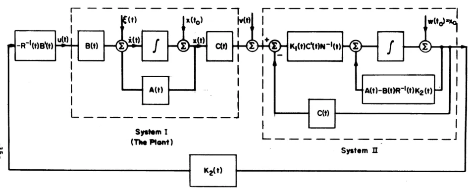
OBSERVATION NOISE AND DRIVING DISTURBANCE

In many cases we do not have exact observation of the states of the system; rather, we observe the output of the system in the presence of measurement noise. In this section, we shall consider the special case when the system is linear and the observation noise is white and Gaussian.

Consider the plant

k(t) = A(t)x(t) + B(t) u(t) + 6(t) (3. 58) y(t) = C(t) x(t) (3.59) where x(t) is an n-vector u(t) is an r-vector A(t) is an n x n matrix B(t) is an n X r matrix

S(t) is an n-vector white Gaussian process C(t) is an mxn matrix

y(t) is an m-vector We observe

s(t) = v(t) + y(t) (3.60)

where v(t) is m-vector white Gaussian process. We shall assume

that we know the statistics of the white Gaussian processes and the initial condition of the plant.

E[ (t)] = 0 ; E[ (t)('(T)] = D(t)S(t-T) _(3.61)

E[ v(t)] = 0 ; E[ v(t)v' (T)] = N(t) 6(t-T) (3. 62) E[g(t)v'(T)] = 0;

E[ x(t

)

'(t)] = 0 ; E[ x(t0)v'(t)] = 0 (3. 63) E[x(t)] =x ₀ E[x(t) - x)(x(t) _{0 0} - x)' ₀ - M (3.64)

0 The cost functional is

t

J = E[<x(t1 ), fx(t )> + <x(t), Q(t)x(t)> + <u(t), R(t)u(t)> dt (3.65) t

0

The problem is to find u(t) to minimize the cost functional (3. 64) subject to the Eq. 3.58. This problem though looks similar to the problem in Section 3.1, it bares a significant difference, namely we don't have exact knowledge of states, thus the simple linear feedback control derived in Section 3. 1 cannot be optimal in this case. We nonetheless shall follow a similar procedure to that used in the pre -vious sections to find the optimal control law.

1. Reformulation of Problem

We first try to fix the form of the optimal control from physical arguments. The maximal information we have about the state of the system at time t is the observation s(t'), for t < t' < t; in order that the control be optimal, it must be a function of the entire ob

-servation s(t'), t0 < t' < t. We wish to incorporate all the available information up to time t in some function of time t; in other words, we like to construct a function w(t) which summarizes all the in-formation contained in s(t'), t _< t' < t, and deduce that the optimal control is of the form

-34-u(t) = g(w(t), t) ; t

<

t

<

t (3.66) Consider a dynamical system with s(t) as the input and w(t)

as the state of the system. Clearly w(t) will summarize all the in-formation of s(t'), t _< t'

<

t. Since s(t) is Gaussian, we also re -quire w(t) to be Gaussian, thus we shall fix the dynamical system to be a linear system with parameter matrices U(t), the feedback gain, and V(t), the forward gain. Therefore we can fix the form of the optimal control to be

u(t) = M(t) w(t) (3.67)

where

<v

(t) = U(t)w(t) + V(t) s(t) (3.68)

We shall assume that Ef w(t)] = E[x(t)] and that the dimension of w(t) equal to the dimension of x(t).t We can view this as a constraint on the form of the system II (see Fig. 2); or, intuitively, we can think of the dynamical system II acting as a filter giving the unbiased estimate of the present state of the plant we are controlling.

Equation 3. 58 implies thatt

rh (t) = A (t)m (t) + B(t)m (t) (3.69)

where

m (t) _x = E[x(t)] ; m (t) _u = E[ u(t)] (3.70) Equations 3. 59, 3. 62, 3. 63 and 3. 68 imply

rh (t)= U(t)mw(t) + V(t)C (t)m (t) (3.71)

tSee Appendix 7. tSee Appendix 2.

--- "_ _I_"I

,

.

.

...

,System

K2(t)

Fig. 2 State-Regulator Problem in the Presence of Disturbing and Observation Noise

K(t) = A (t) K I(t)+ K,(t)A'(t) - Kj(t)C'(t)N~I(t)C(t)K 1(t) + D(t)

-K₂(t) = A'(t)K2(t)+ K2(t)A(t) -K 2(t)B(t)R (t)B'(t)K2(t)+Q(t)

-36-where

m w(t) = E[w(t)]

By Eq. 3. 67, (3. 69) yields

rh (t) = A(t)m (t) + B(t)M(t)m, The unbiasness assumption gives us

[A(t) - U (t) - V(t) C(t) + B(t)M(t)] m (t) = 0

This is true for all m (t) ' 0, thus (3.74) implies

U(t) = A(t) - V(t) C(t) + B(t)M(t)

We see that the unbiasness assumption places a constraint on the parameters of the dynamical system II by Eq. 3. 75.

the composite vectors

x(t) z (t) = ,... w(t)_

; (t) ...

v (t). Let us define (3.76)

Equations 3.58, 3.59, 3.60, 3.67, 3.68 and 3. 75 imply that

z(t) = S(t) z(t) + Y(t) ,1(t) where

~ A(t)

S(t) = ... V t) C(t) B(t)M(t) .C... : A(t) - V (t) C (t) + I .0

Y(t)

=

..

o

V(t)

(3.72) (3.73) (3.74) (3.75) (3.77) (3.78) (3.79)

V

-37-and the statistics of n(t) are

E[ (t)] = 0

; E

[n(t) n'(-r)] = X(t) 5(t--)

where

and E [ z(t)'(t)] = 0 ; to

<

t

<

t

By Appendix 2, Eqs. 3.77 together with 3.81, 3.82 imply that

Z z(t) = S(t) Z z(t) + Z z(t) S' (t) + Y(t) X(t) Y '(t)z where we define (3.83) E (t . E (t)

wx

.w

(3.84)

The cost functional (3. 64) can be written as

J = Tr[FE (t₁) + (3.85)

The new optimization problem is: (3.85), choose M(t), V(t)

given (3. 83) and the cost functional such that (3. 85) is minimized subject to the matrix differential equation (3.83).

2. Application of the Matrix Minimum Principle Let the costate matrix of Zz(t) be Pz(t) where

S(t). Pxw (t) Pz(t) = . .' ... P

_{(t)'. Pw}

_t

(3 . 80 (3.81) (3.82) (3.86) Q (t)

F

(t) + M'(t)R(t)M(t) w (t) dt] I D(t) .0 X (t)= ... '. .... O '. N(t)j

-38-Therefore the costate matrices for Z (t), w(t), wx (t) and Exw(t)

are P (t), P w(t), P wx(t) and P xw(t) respectively. We form the Hamiltonian

H = Tr[ (t) P'(t) + Q(t) E (t) + M'(t) R(t) M(t) Zw(t)] (3.87)

The canonical equations for the costate yields:

* ' ** * -P = A'(t)P (t)+C'(t)V (t) P (t) +P (t)A(t) + (t)V (t)C(t)+ Q(t) x x wx xx (3.88) -P (t) = A'(t)Pxw(t) + C'I(t) V (t) Pw(t) + P (t) B(t) M (t) + Pxw(t) A (t) P (t)V (t C t) +

Px

B (t) M (t) (3 . 89) '* * 1* * *' *. -P (t) = A'(t)P C'(t)Vt)P )+- (t) + M (t)B'(t)wx(t) wxww +M (t) B(t) (t) + P (t) A (t) + P(t) V (t) C(t) (3.90) ' *' * *' * -P (t) M (t)P (t) + t)P (t) + M '(t)BIM t)P (t) wx wx w wx *1* * * * +M (t)BtPw( P (t) + P (t)B(t)M (t) + P (t) A (t) x wx w *J- * *j *' * P (t) V ()C (t)t) + A)(t) (t) + M?(t)R (t)M (t) (3.91) w w w

The transversality conditions give the boundary conditions

*1* * *

P (t )PF ; P (t P Px(tM) Pw(t) 0 (3.92)

w xw xw

By Eqs. 3. 89, 3. 90, 3. 91 and 3. 92, we deduce that

* *' * *'

Pw(t) + =P (t)MtM (3.93)

tonian, H(E'(t), Pz(t), M(t), dependently, we set

V(t)) with respect to V(t) and M(t)

in-8V(t) z(t)

S [t)[F (t),

P (t), M(t),

P (t), M(t),

Differentiating (3.78) with respect to V(t) and M(t), respectively, (3. 94) and (3. 95) yield -C * * *P *( * * * PIt), t 't P (t) (t) C'I(t) + P (t E t(t) t) - P (t) f" (t) C' (t) wX X wX Xw w wX w w +P (t) V (t) N(t) = 0 w (3.96) B'(t)P (t) F (t) + B'(t)P' (t) (t) + B'(t)P (t)E (t) x xw xw w wx xw + B'(t)P (t)E (t) + R(t)M'(t)E (t) _{w w w} = 0 (3.97) By assumption, N(t) and R(t) are positive definite, therefore the

* *

Eqs. 3. 94 and 3. 95 give the values of M (t) and V (t) which mini-mize the Hamiltonian.

By assumption and 3. 92 imply that

w (t), Pw(t)

N(t), R(t) are nonsingular, and Eqs. 3. 91 is nonnegative definite;t thus Eqs. 3. 96 and

3. 97 yield

-1 -1It

V (t = P *-I (t) P _{w wx} (t)[IFsE _xw (t) - f' (t)]I C'I(t) N~I(t) + [ _{x w} (t) - E* (t)] C'I(t)N~ (t_wx

(3.98)

fIf M (t) is nonzero, then P (t) is positive definite for t / t

w 0

= 0 (3.94)

V(t)]

V(t)] = 0 (3.95)

Hamil-Z(t) z 0 P'(t₁ ) =

+

+

xx

0 0

x

x

0 0

F

0]

LO : (3.100) (3.101)

Formally, we can solve the resulting matrix differential equations for 2z(t) and P (t), and substitute the solution into (3. 98) and (3. 99) to_{z z} obtain V'(t) and M*(t). However, it can be shown that T the solution that satisfies the resulting matrix differential equation and the

cor-responding boundary conditions is of the form

S ( P (t = -P (t)

xw w xw xw (3. 102)

By the uniqueness theorem, (3. 102) is the form of the solution we are interested in. Substituting (3.102) into (3. 97) and (3. 98), we have

V (t = [E ()- _x *(t]C (t) N -(t)_w *I -1 * * M (t) = -R (t)B'(t)[P'(t) _x - P (t)] w (3. 103) (3. 104) tSee Appendix 5.

fSee Appendix 5, Eqs. A. 5. 16, A. 5. 17, A. 5. 1 and A. 5. l.

-40-M~ -R (t) B (t)~I~r

M (t) =-R- (t)B'(t)[ _X (t)+P _wX (t)]1E _xw (t) E _w t) - R- tB ()P _xw (t) +P _w(t)]

(3.99) Substituting (3. 98) and (3. 99) into (3. 90), (3. 91), (3. 88), (3. 83) we have a set of matrix differential equationsT of 2? (t) and P (t) with

b cz boundary conditions x x' o o x x o o