HAL Id: hal-01806708
https://hal.archives-ouvertes.fr/hal-01806708
Submitted on 12 Jun 2018
HAL is a multi-disciplinary open access
archive for the deposit and dissemination of
sci-entific research documents, whether they are
pub-lished or not. The documents may come from
teaching and research institutions in France or
abroad, or from public or private research centers.
L’archive ouverte pluridisciplinaire HAL, est
destinée au dépôt et à la diffusion de documents
scientifiques de niveau recherche, publiés ou non,
émanant des établissements d’enseignement et de
recherche français ou étrangers, des laboratoires
publics ou privés.
complexity model to the different climate configurations
of the last nine interglacials
Nathaëlle Bouttes, Didier Swingedouw, Didier Roche, Maria Sanchez-Goni,
Xavier Crosta
To cite this version:
Nathaëlle Bouttes, Didier Swingedouw, Didier Roche, Maria Sanchez-Goni, Xavier Crosta. Response
of the carbon cycle in an intermediate complexity model to the different climate configurations of the
last nine interglacials. Climate of the Past, European Geosciences Union (EGU), 2018, 14 (2), pp.239
- 253. �10.5194/cp-14-239-2018�. �hal-01806708�
https://doi.org/10.5194/cp-14-239-2018
© Author(s) 2018. This work is distributed under the Creative Commons Attribution 3.0 License.
Response of the carbon cycle in an intermediate
complexity model to the different climate
configurations of the last nine interglacials
Nathaelle Bouttes1, Didier Swingedouw1, Didier M. Roche2,3, Maria F. Sanchez-Goni1,4, and Xavier Crosta1
1Univ. Bordeaux, EPOC, UMR 5805, 33615 Pessac, France
2Laboratoire des Sciences du Climat et de l’Environnement, LSCE/IPSL, CEA-CNRS-UVSQ,
Université Paris-Saclay, 91191 Gif-sur-Yvette, France
3Earth and Climate Cluster, Faculty of Science, Vrije Universiteit Amsterdam, Amsterdam, the Netherlands 4EPHE, PSL Research University, 33615 Pessac, France
Correspondence:Nathaelle Bouttes (nathaelle.bouttes@lsce.ipsl.fr) Received: 28 October 2016 – Discussion started: 8 November 2016
Revised: 16 November 2017 – Accepted: 6 December 2017 – Published: 2 March 2018
Abstract.Atmospheric CO2levels during interglacials prior
to the Mid-Brunhes Event (MBE, ∼ 430 ka BP) were around 40 ppm lower than after the MBE. The reasons for this dif-ference remain unclear. A recent hypothesis proposed that changes in oceanic circulation, in response to different exter-nal forcings before and after the MBE, might have increased the ocean carbon storage in pre-MBE interglacials, thus low-ering atmospheric CO2. Nevertheless, no quantitative
esti-mate of this hypothesis has been produced up to now. Here we use an intermediate complexity model including the car-bon cycle to evaluate the response of the carcar-bon reservoirs in the atmosphere, ocean and land in response to the changes of orbital forcings, ice sheet configurations and atmospheric CO2concentrations over the last nine interglacials. We show
that the ocean takes up more carbon during pre-MBE in-terglacials in agreement with data, but the impact on atmo-spheric CO2is limited to a few parts per million. Terrestrial
biosphere is simulated to be less developed in pre-MBE inter-glacials, which reduces the storage of carbon on land and in-creases atmospheric CO2. Accounting for different simulated
ice sheet extents modifies the vegetation cover and tempera-ture, and thus the carbon reservoir distribution. Overall, at-mospheric CO2levels are lower during these pre-MBE
sim-ulated interglacials including all these effects, but the mag-nitude is still far too small. These results suggest a possible misrepresentation of some key processes in the model, such as the magnitude of ocean circulation changes, or the lack of crucial mechanisms or internal feedbacks, such as those
related to permafrost, to fully account for the lower atmo-spheric CO2concentrations during pre-MBE interglacials.
1 Introduction
Ice core data have shown that atmospheric CO2
concen-tration has been different during interglacials of the last 800 000 years (Lüthi et al., 2008; Bereiter et al., 2015). Older interglacials before the Mid-Brunhes Event (MBE) around 430 ka BP, i.e. Marine Isotope Stages (MIS) 13, 15, 17 and 19, are characterised by relatively lower atmospheric CO2,
around 240 ppm, compared to more recent interglacials, i.e. MIS 1, 5, 7, 9 and 11, which have a higher CO2 level of
around 280 ppm (Fig. 1a).
Proxy data such as the marine benthic foraminifera δ18O stack record, embedding both deep-sea temperature and ice sheet volume (Lisiecki and Raymo, 2005), indicate that older interglacials (pre-MBE) experienced a colder climate than the more recent ones (post-MBE). This tendency is also supported by individual δ18O and sea surface temperature (SST, derived from Mg/Ca paleothermometry, alkenones or foraminifera assemblages) records from marine sediment cores (Lang and Wolff, 2011; Past Interglacials Working Group of PAGES, 2016), although some individual sub-stages such as MIS 7c and 7e were colder than the post-MBE mean interglacial climate.
Figure 1.(a) Atmospheric CO2(ppm) record at EPICA Dome C (Lüthi et al., 2008) and insolation (W m−2) (b) at 65◦N on 21 June and (c) at 65◦S on 21 December, based on Berger (1978).
To explain the different climates of interglacials before and after the MBE, modelling studies have shown that it is necessary to include the change of atmospheric CO2 (Yin
and Berger, 2010, 2012). Indeed, these numerical simula-tions with an intermediate complexity model have demon-strated that differences in Earth’s orbital configuration, and hence seasonal and spatial distribution of insolation, alone cannot explain the colder climate recorded during pre-MBE interglacials, whereby lower atmospheric CO2concentration
is also necessary to simulate colder climate (Yin and Berger, 2010, 2012). However, the reasons for the lower CO2values
remain elusive and very few modelling exercises have tack-led the issue of different CO2levels during interglacials
be-fore and after the MBE. Köhler and Fischer (2006) have pro-duced transient simulations of the last 740 000 years using the BICYCLE box model. They used several paleoclimatic records such as ocean temperature, sea ice, sea level, ocean circulation, marine biota, terrestrial biosphere and CaCO3
chemistry to force their model forward. They run a set of simulations prescribing only one forcing at a time and an-other with all forcings excluding one at a time, which allows them to analyse which forcings are the most important. In their simulations, they have shown that the lower CO2
val-ues during pre-MBE are mainly explained by the prescribed lower Southern Ocean sea surface temperature and weaker Atlantic meridional overturning circulation (low North At-lantic Deep Water formation and Southern Ocean vertical mixing) compared to post-MBE interglacials. Using an
inter-mediate complexity model, Yin (2013) conversely simulated vigorous bottom water formation and stronger ventilation in the Southern Ocean during pre-MBE interglacials and sug-gested this could increase deep oceanic carbon storage and lower atmospheric CO2. However, this effect on the ocean
carbon reservoir and atmospheric CO2has not been
evalu-ated yet in a climate model including a carbon cycle repre-sentation.
Changes in surface temperature also modify the partition of the carbon cycle: in the ocean, colder SST increases the solubility of CO2, increasing its potential uptake from the
at-mosphere during pre-MBE interglacials. In contrast, on land a colder climate might yield a decrease in biomass, reduc-ing CO2 uptake via lower continental carbon storage.
Be-cause the ice sheets in the Northern Hemisphere are differ-ent during the interglacials in response to the differdiffer-ent values of CO2 and orbital configurations (Ganopolski and Calov,
2011), they might also have an impact on the carbon cycle, for example by modifying the terrestrial biosphere extent.
Here, we test the impact of the different orbital configura-tions of the last nine interglacials on the carbon cycle. For this purpose, we use a coupled carbon–climate model to evaluate the changes of carbon storage in the ocean and in the terres-trial biosphere, as well as the impact of different Northern Hemisphere ice sheet volumes.
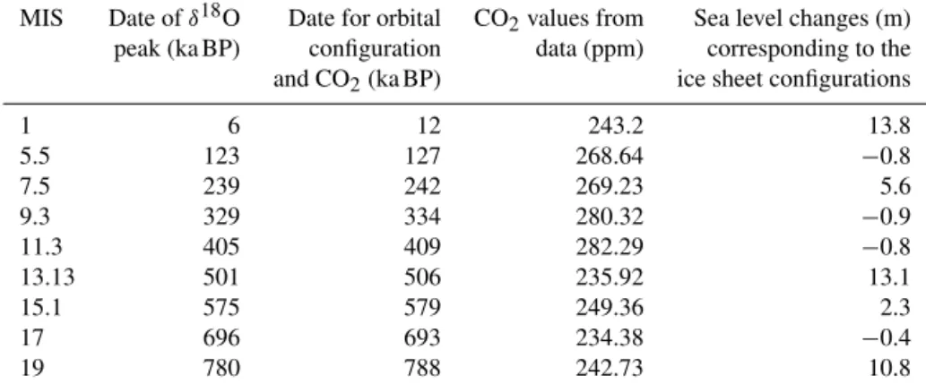
Table 1.Dates of orbital parameters and CO2used for the simulations (Lüthi et al., 2008), and sea level anomalies as compared to present-day conditions (m) corresponding to the prescribed ice sheets (Ganopolski and Calov, 2011).
MIS Date of δ18O Date for orbital CO2values from Sea level changes (m) peak (ka BP) configuration data (ppm) corresponding to the and CO2(ka BP) ice sheet configurations
1 6 12 243.2 13.8 5.5 123 127 268.64 −0.8 7.5 239 242 269.23 5.6 9.3 329 334 280.32 −0.9 11.3 405 409 282.29 −0.8 13.13 501 506 235.92 13.1 15.1 575 579 249.36 2.3 17 696 693 234.38 −0.4 19 780 788 242.73 10.8 2 Methods
We use the iLOVECLIM climate model of intermediate com-plexity, which is a new development branch (code fork) of the LOVECLIM model in its version 1.2 (Goosse et al., 2010). iLOVECLIM has an atmosphere module (ECBILT) with a T21 spectral grid truncation (∼ 5.6◦ in latitude–longitude in the physical space) and three vertical layers. The ocean component (CLIO) has a horizontal resolution of 3◦ by 3◦ and 20 vertical levels. The evolution of the terrestrial bio-sphere, i.e. the proportion of desert, grasses and tree cover, is computed by the VECODE model (Brovkin et al., 1997). It includes a carbon cycle module on land and in the ocean (Bouttes et al., 2015). iLOVECLIM is an evolution from the LOVECLIM model used in previous model studies of the last nine interglacials focused on climate (Yin and Berger, 2010, 2012; Yin, 2013). It has the same atmospheric and oceanic modules but includes a different carbon cycle representation in the ocean (Bouttes et al., 2015). We have chosen the same dates for the nine orbital configurations as in Yin and Berger (2010, 2012) and Yin (2013), i.e. the maximum of insolation preceding the δ18O peak values (Table 1, Fig. 1b and c). Con-trary to most simulations from these studies, we also use the CO2values (as well as CH4and N2O) at the same dates as
for the orbital configurations (and not at the CO2peak), but
as stated in Yin and Berger (2012), this may not affect the main results concerning the simulated climatic changes.
In the model, we separate the atmospheric CO2
concen-tration into two distinct variables depending on its physical and chemical impact. The first one is used in the radiative scheme of the atmosphere, for which we prescribe the CO2
from measured values in all the described simulations (Lüthi et al., 2008; Fig. 1a). Another atmospheric CO2is computed
interactively in the model as a result of the balance of the carbon fluxes between the different carbon subcomponents (atmosphere, ocean and terrestrial biosphere). We make this choice of keeping the two separated to ensure that the cli-mate simulated by the model is coherent with past measured
atmospheric CO2. In other words, we consider the
atmo-spheric CO2 concentration as an imposed external forcing,
while within the carbon cycle the atmospheric CO2
concen-tration is allowed to vary but does not impact the atmospheric radiative forcing. By doing this, we limit the number of de-grees of freedom in our climate carbon system, which no-tably allows us to avoid the complication arising from sim-ulating a different climate when the climate and carbon are fully coupled.
The simulations performed are snapshots, run with con-stant orbital and atmospheric CO2concentration forcing and
integrated over 3000 years, allowing the ocean to reach a quasi-equilibrium. All simulations start from the pre-industrial control one, and the average of the last 100 years is used to analyse the results.
Our strategy is to evaluate the impact of the different cli-mate and carbon compartments to set the atmospheric CO2
concentration. For this purpose, we consider three series of simulations, which have all been run for the nine interglacials (Table 2). The first series (“Ocean Carbon”, OC) has fixed ice sheets set to the observed pre-industrial ones and a fixed terrestrial biosphere set to the simulated pre-industrial one. This first set of simulations thus provides the response of the ocean alone to the different orbital parameters and CO2
lev-els of the nine interglacials. The second series (“Ocean Veg-etation Carbon”, OVC) still has fixed ice sheets but includes an interactive terrestrial biosphere, computed by the model. It gives the response of both the ocean and land vegetation reservoirs to the different orbital parameters and CO2as well
as their interactions for setting the atmospheric CO2
concen-tration. Finally, the third series (“Ocean Vegetation Ice sheet Carbon”, OVIC) has different prescribed ice sheets in the Northern Hemisphere for the nine interglacials. The ice sheet distribution change is based on modelling results, given that the uncertainty from data is very large for the interglacials of the last 800 000 years, especially the oldest ones. The pre-scribed ice sheet distributions are thus taken from an ice sheet simulation of the last 800 000 years (Ganopolski and Calov,
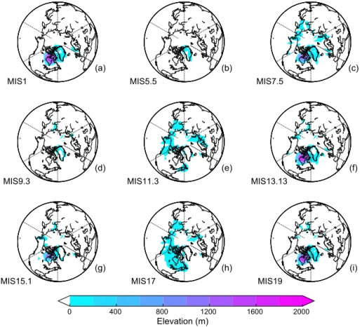
MIS1 (a) MIS5.5 (b) MIS7.5 (c) MIS9.3 (d) MIS11.3 (e) MIS13.13 (f) MIS15.1 (g) MIS17 (h) MIS19 (i) 0 400 800 1200 1600 2000 Elevation (m)
Figure 2.Ice sheet elevation (m) in the Northern Hemisphere simulated by the CLIMBER-2 model (Ganopolski and Calov, 2011) and used in the OVIC series for each interglacial simulation, in anomalies with respect to the pre-industrial elevation.
Table 2.Summary of the three series of simulations.
Name of the series Components impacting the carbon cycle Ocean Vegetation Different interglacial ice sheets
OC X × ×
OVC X X ×
OVIC X X X
2011) using the intermediate complexity model CLIMBER-2 (Petoukhov et al., CLIMBER-2000; Ganopolski et al., CLIMBER-2001; Brovkin et al., 2002), including a 3-D polythermal ice sheet model (Greve, 1997). This ice sheet model is coupled to the cli-mate component via surface energy and mass balance inter-face (Calov et al., 2005), which accounts for the effect of aeolian dust deposition on snow albedo. The ice sheet distri-bution is chosen 2000 years after the chosen interglacial date to account for the long timescale of the ice sheet response during a deglaciation and to ensure that the ice sheet corre-sponds to an interglacial configuration. The ice sheet eleva-tions for the nine interglacial simulaeleva-tions are shown in Fig. 2 and the corresponding sea level change in Table 1. The ter-restrial biosphere is also interactive in this OVIC series of simulations. This last set of simulations thus adds the effect
of having different ice sheets in the Northern Hemisphere for the carbon cycle variations.
3 Results and discussion
3.1 Role of the ocean (OC simulations)
Similar to previous numerical studies of the interglacials with the LOVECLIM model (Yin and Berger, 2010, 2012), the changes in orbital configuration and atmospheric CO2altered
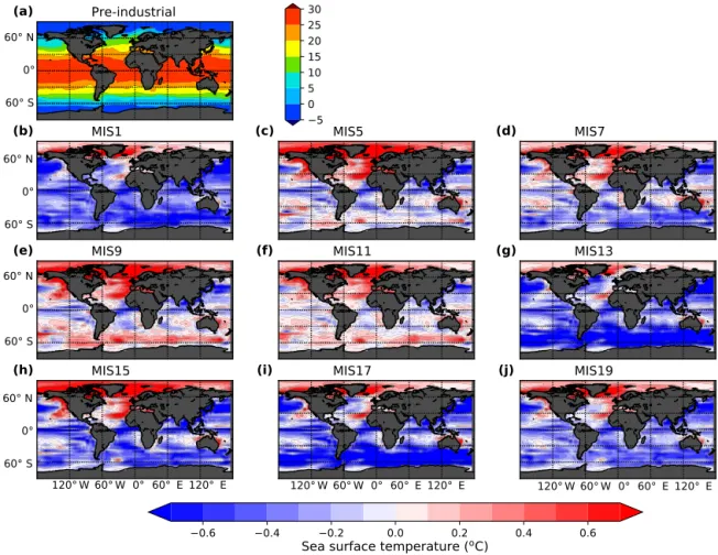
SSTs and oceanic circulation for each interglacial simulation of the OC series. All simulations have warmer SSTs than the control pre-industrial in the Northern Hemisphere high latitudes (Fig. 3). Except for MIS 1, the SSTs in the post-MBE simulations (corresponding to MIS 5, 7, 9 and 11) are
60° S 0° 60° N Pre-industrial (a) 5 0 5 10 15 20 25 30 MIS1 (b) (c) MIS5 (d) MIS7 MIS9
(e) (f) MIS11 (g) MIS13
120° W 60° W 0° 60° E 120° E
MIS15
(h) (i) MIS17 (j) MIS19
0.6 0.4 0.2 0.0 0.2 0.4 0.6
Sea surface temperature (oC)
60° S 0° 60° N 60° S 0° 60° N 60° S 0° 60° N 120° W 60° W 0° 60° E 120° E 120° W 60° W 0° 60° E 120° E
Figure 3.Annual SST (◦C) in (a) the pre-industrial control simulation and (b–j) the interglacial simulations of the OC series with fixed vegetation and fixed ice sheets, in anomalies with respect to the pre-industrial control simulation.
Table 3.SST data (◦C) from the Past Interglacials Working Group of PAGES (2016) and shown in Figs. 4a and b and 14.
Latitude (◦) Longitude (◦) Site MIS 5e MIS 7e MIS 9e MIS 11c MIS 13a MIS 15a MIS 17c MIS 19c post-MBE pre-MBE Difference pre- and post-MBE 57.51 −15.85 ODP 982 16.2 14.5 15.8 15 13.7 14.1 14.2 14.1 15.4 14.0 −1.35 56.04 −23.23 DSDP 552s 15.1 14.7 14.2 16.4 12.4 14.7 18.3 14.7 15.1 15.0 −0.08 41.01 −126.43 ODP 1020 14.1 11.7 12.8 14 10.2 12.5 13.6 12.1 13.2 12.1 −1.05 41.00 −32.96 DSDP 607s 25.1 20.5 23.6 26.8 22.3 20.3 25.2 24 24 23.0 −1.05 32.28 −1148.40 ODP 1012 19.5 17.7 19.7 19.1 17.5 18.3 19.3 18 19 18.3 −0.73 19.46 116.27 ODP 1146 27.3 26.3 27.3 26.8 26.1 26.3 26.9 26.2 27.0 26.4 −0.55 16.62 59.80 ODP 722 27.7 27.3 27.5 27.5 27 27.1 27.2 27.2 27.5 27.1 −0.38 9.36 113.29 ODP 1143 28.8 27.8 28.6 28.3 28.4 28.1 28.6 28.2 28.4 28.3 −0.05 2.04 141.76 MD97-2140 29.5 28.6 29 29.5 28.6 28.4 29.3 28.9 29.2 28.8 −0.35 0.32 159.36 ODP 806B 29.6 29.2 28.8 30.2 28.2 29.4 29 29.4 29.5 29 −0.45 −3.10 −90.82 ODP 846 25.1 24 23.8 24 23.6 23.7 23.7 23.7 24.2 23.7 −0.55 −41.79 −171.50 ODP 1123 17.7 19 19.6 19.3 17.8 18.8 18 17.9 18.9 18.1 −0.78 −42.91 8.9 ODP 1090 17.1 10.2 14.7 13.9 10.2 11.7 11.1 10.4 14.0 10.9 −3.125 −43.45 167.9 MD06-2986 18 16.5 16.6 18.1 15.5 16.2 16.3 15.8 17.3 16.0 −1.35 −45.52 174.95 DSDP594 18.3 7.1 9.5 17.5 10 11.7 12.1 9.7 13.1 10.9 −2.23
also warmer than in the pre-industrial control in large areas in the Northern Hemisphere mid-latitudes. In the MIS 5, 9 and 11 simulations the SSTs are slightly warmer in the South-ern Ocean. In the pre-MBE simulations (MIS 13, 15, 17 and 19), the ocean is mainly colder than the pre-industrial ocean, especially in the Southern Hemisphere. To compare the pre-MBE to post-pre-MBE simulations, we built a composite
(av-erage) for each period (pre- and post-MBE). We have ex-cluded MIS 1 from the post-MBE composite, for which the date chosen corresponds to a CO2much lower than the other
post-MBE interglacials. We thus consider MIS 5, 7, 9 and 11 in the post-MBE composite and MIS 13, 15, 17 and 19 in the pre-MBE composite. The difference between the pre- and post-MBE composites shows colder SSTs in the pre-MBE
(a)
(c)
(e)
(b)
(d)
(f)
-1 -1Figure 4.(a, b) Annual SST difference (◦C), (c, d) meridional overturning circulation difference (Sv) and (e, f) dissolved inorganic carbon difference (µmol kg−1) between pre-MBE (MIS 13, 15, 17, 19) and post-MBE (MIS 5, 7, 9, 11) interglacial simulations for (a, c, e) the OC series with fixed vegetation and fixed ice sheets and (b, d, f) the OVC series with interactive vegetation and fixed ice sheets. The vertical black line indicates the limit between the Southern Ocean south of 32◦S and the Atlantic Ocean north of 32◦S. The dots in panel (a) are SST data differences based on the Past Interglacials Working Group of PAGES (2016) (Table 3).
interglacial simulations compared to the post-MBE simula-tions, especially in the Southern Ocean (Fig. 4a). The differ-ence in global mean simulated SST is −0.30◦C, reaching up to −0.36◦C in the North Atlantic (between 30 and 65◦N)
and −0.43◦C in the Southern Ocean (south of 54◦S). This
is in general agreement with SST data, which indicate colder SSTs in the pre-MBE interglacial oceans, especially in the Southern Ocean (Table 3, Fig. 4a), although the comparison is limited by the lack of SST records across the MBE.
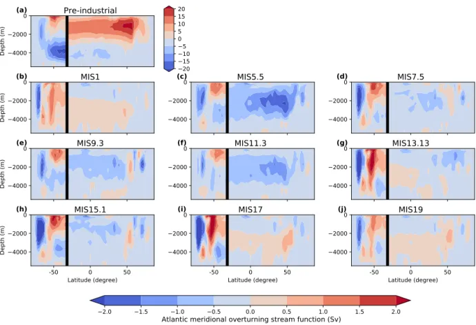
Compared to the pre-industrial period, the ventilation of the Southern Ocean is increased in all simulations (Fig. 5).
The formation of Antarctic Bottom Water (AABW) as well as the wind-driven meridional cell between 40 and 60◦S (so-called Deacon cell) are both stronger. On average, the maximum of the Deacon cell is increased by 7 % between pre- and post-MBE simulations, while AABW is increased by 18 % (Fig. 4c). The meridional overturning circulation is also slightly increased by 6 % and deepened in the At-lantic Ocean. All these results concerning oceanic circula-tion changes are very similar to those of Yin et al. (2013), allowing us to test their hypothesis on the impact of these
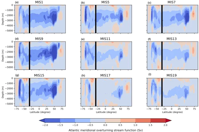
4000 2000 0 Depth (m) Pre-industrial (a) 20 15 10 5 0 5 10 15 20 4000 2000 0 Depth (m) MIS1 (b) 4000 2000 0 MIS5.5 (c) 4000 2000 0 MIS7.5 (d) 4000 2000 0 Depth (m) MIS9.3 (e) 4000 2000 0 MIS11.3 (f) 4000 2000 0 MIS13.13 (g) -50 0 50 Latitude (degree) 4000 2000 0 Depth (m) MIS15.1 (h) -50 0 50 Latitude (degree) 4000 2000 0 MIS17 (i) -50 0 50 Latitude (degree) 4000 2000 0 MIS19 (j) 2.0 1.5 1.0 0.5 0.0 0.5 1.0 1.5 2.0
Atlantic meridional overturning stream function (Sv)
Figure 5.Meridional overturning circulation (Sv) in the Southern Ocean and in the Atlantic Ocean north of 32◦S in (a) the pre-industrial control simulation and (b–j) the interglacial simulations of the OC series with fixed vegetation and fixed ice sheets, in anomalies with respect to the pre-industrial control simulation. The vertical black line indicates the limit between the Southern Ocean south of 32◦S and the Atlantic Ocean north of 32◦S.
changes on ocean carbon uptake and atmospheric CO2
con-centrations.
The changes in global ocean circulation and SST mod-ify the carbon storage in the ocean. The colder SST, which increases dilution of CO2 at the ocean surface, associated
with stronger ventilation in the pre-MBE simulations yields a larger carbon uptake by the ocean. Such processes result in higher dissolved inorganic carbon (DIC) concentrations in the Southern Ocean, as well as higher DIC concentration in the upper ocean (first 2 km of the ocean) (Fig. 4e), reflect-ing the average increase of 4.7 Gt C in pre-MBE simulations. Conversely, the DIC slightly decreases in the deeper ocean, which may be due to the increased ventilation of North At-lantic Deep Water bringing more carbon back from the deep ocean to the surface.
The stronger uptake of carbon by the ocean leads to a de-crease in atmospheric CO2 concentration during the
pre-MBE interglacials compared to the post-pre-MBE ones (Fig. 6), in agreement with CO2data as shown by the very good
corre-lation between the measured and simulated values (r = 0.91, p <0.01; Fig. 6). However, the difference in magnitude be-tween pre- and post-MBE values is only a few parts per mil-lion in the simulations. Thus, even though simulations
quali-230 240 250 260 270 280 290 Measured atmospheric CO2(ppm) 275 276 277 278 279 280 281 Simulated atmospheric CO 2 (ppm) MIS1 MIS5 MIS7 MIS9 MIS11 MIS13 MIS15 MIS17 MIS19 r = 0.91,p = 0.00077 y = 0.07 x + 259.28
Figure 6.Simulated CO2in the interglacial simulations of the OC series as a function of the measured CO2from data (Lüthi et al., 2008). The Pearson correlation coefficient and the p value are indi-cated at the top.
tatively reproduce the geological CO2trend, with lower
the magnitude of the difference is much lower in the sim-ulation (∼ 1–5 ppm) than in the data (∼ 30–40 ppm). In fact, the slope of the linear regression between simulated and ob-served atmospheric CO2concentration is 0.07, indicative of
a ∼ 14-fold underestimation by the simulations.
Hence the ocean carbon uptake in the simulations is not sufficient to drive a significant lowering of atmospheric CO2.
Either the change in global ocean circulation and SST should be larger or another mechanism and feedbacks need to be taken into account to modify the biological or physical car-bon uptake and amplify the initial change. Since the repre-sentation of bottom water formation in the Southern Ocean is biased in the model, with an over-representation of open ocean convection, as is also the case for many more complex general circulation models (Heuzé et al., 2013), it is possi-ble that this hinders simulating the full range of carbon stor-age due to ocean circulation changes, as it is suspected for colder periods such as the Last Glacial Maximum (around 21 000 years ago) (Fischer et al., 2010).
3.2 Role of land vegetation and soils (OVC simulations) In the first series of simulations, solely the ocean was allowed to respond to the different external forcings while land vege-tation and soils were fixed to their pre-industrial distribution. To account for changes in land vegetation and soils on the carbon cycle, a second series of simulations (OVC) was con-ducted with an interactive terrestrial biosphere module on top of the ocean’s module (Table 2).
Compared to the pre-industrial control simulation, more trees develop in North Africa and the southern part of Eura-sia in these interglacial simulations, while the tree cover is reduced in central North America and some regions in the northern part of Eurasia (Fig. 7). When compared to OC sim-ulations with fixed vegetation, the OVC simsim-ulations demon-strate a surface ocean warming almost everywhere except in the North Atlantic for some interglacials (Fig. 8). In re-sponse to the global warmer surface ocean, the stratification in the convection region in the North Atlantic increases (e.g. Swingedouw et al., 2007a) leading to a slowdown of the At-lantic meridional oceanic circulation, especially for MIS 1, 5 7, 9 and 15 (Fig. 9).
For the carbon cycle, the activation of the terrestrial mod-ule results in more carbon stored in land vegetation and soils for all interglacial simulations (Fig. 10b) since the vegeta-tion cover increases compared to the control because of the warmer climate. This tends to lower atmospheric CO2
con-centration, hence the pCO2 difference at the air–sea
inter-face, leading to an outgassing of carbon from the ocean to the atmosphere, which ultimately decreases the storage of carbon in the ocean. The ocean carbon storage is also dimin-ished compared to the series of simulations with fixed vege-tation due to the warmer ocean temperature, which reduces the CO2 solubility in water. The increase in carbon storage
in the terrestrial biosphere is generally larger than the loss of
carbon from the ocean so that the carbon content of the at-mosphere is also diminished in these simulations compared to the fixed vegetation simulations, and atmospheric CO2is
slightly lower or not changed (Fig. 11a).
In terms of difference between pre- and post-MBE inter-glacial simulations, we find less vegetation cover in most ar-eas (except in North Africa and parts of south Eurasia) and consequently less carbon stored (−48 Gt C) in land vegeta-tion and soils in the pre-MBE simulavegeta-tions compared to post-MBE simulations (Fig. 12). This effect tends to increase at-mospheric CO2on average in pre-MBE interglacial
simula-tions.
For the ocean, the differences between pre- and post-MBE simulations are similar to the ones for the simulations with fixed vegetation (OC). On average, the SST is lower in the pre-MBE simulations compared to post-MBE simula-tions (−0.28◦C globally, −0.31◦C in the North Atlantic and
−0.44◦C in the Southern Ocean) except in a small area in
the North Atlantic (Fig. 4b), and the ventilation is increased in the pre-MBE simulations (Fig. 4d). Hence the ocean can store more carbon in the pre-MBE simulations than the post-MBE simulations with an average increase in carbon storage in the pre-MBE ocean of 43 Gt C compared to the post-MBE ocean. Similarly, the DIC concentration is higher in pre-MBE simulations, especially in the upper ocean and deep South-ern Ocean, as in the previous series of simulations with fixed vegetation (Fig. 4f).
As the diminution in land carbon storage is larger than the increase in ocean carbon storage, more carbon is con-served in the atmosphere resulting in higher CO2on average
for the pre-MBE simulations than the post-MBE simulations (Fig. 11b). There is thus a qualitative disagreement (nega-tive correlation of −0.33 (p = 0.38) between simulated and observed atmospheric CO2for the interglacials considered)
with the observations.
Nevertheless, it should be noted that permafrost (frozen soil) was not taken into account in these simulations. If there was more permafrost during the colder pre-MBE in-terglacials, it could store more carbon on land and counteract the loss of carbon due to the reduction of vegetation cover and production (Crichton et al., 2016).
Comparison with pollen data (Table 4) indicates that the model is in qualitative agreement with reconstructed tree cover change in South America where the tree cover was smaller on average in pre-MBE than in post-MBE inter-glacials (Fig. 12a). In southern Europe, the tree fraction data indicate that on average slightly more tree cover prevailed during pre-MBE than during post-MBE interglacials, also in agreement with simulations, although the variability in the data among interglacials is large.
3.3 Impact of different ice sheets (OVIC simulations) The last series of simulations (OVIC) has the same design as OVC but also takes into account possible differences in ice
Figure 7.Tree cover (%) change with respect to the pre-industrial control simulation for the OVC series with interactive vegetation and fixed ice sheets.
60° S 0° 60° N
MIS1
MIS5
MIS7
60° S 0° 60° N
MIS9
MIS11
MIS13
60° S 0° 60° N
120° W 60° W 0° 60° E 120° E
MIS15
MIS17
MIS19
0.4 0.2 0.0 0.2 0.4
Sea surface temperature (
oC)
120° W 60° W 0° 60° E 120° E 120° W 60° W 0° 60° E 120° E
5000 4000 3000 2000 1000 0 Depth (m)
MIS1
MIS5
MIS7
5000 4000 3000 2000 1000 0 Depth (m)
MIS9
MIS11
MIS13
75 50 25 0 25 50 75 Latitude (degree) 5000 4000 3000 2000 1000 0 Depth (m)
MIS15
75 50 25 0 25 50 75 Latitude (degree)MIS17
75 50 25 0 25 50 75 Latitude (degree)MIS19
2.0 1.5 1.0 0.5 0.0 0.5 1.0 1.5 2.0Atlantic meridional overturning stream function (Sv)
Figure 9.Meridional overturning circulation difference (Sv) between simulations with interactive vegetation (OVC) and with fixed vegeta-tion (OC). The vertical black line indicates the limit between the Southern Ocean south of 32◦S and the Atlantic Ocean north of 32◦S.
MIS1 MIS5 MIS7 MIS9 MIS11 MIS13 MIS15 MIS17 MIS19 15 10 5 0 5 10 15 Carbon stocks (GtC) (a) Atmosphere Ocean Land
MIS1 MIS5 MIS7 MIS9 MIS11 MIS13 MIS15 MIS17 MIS19 200 100 0 100 200 Carbon stocks (GtC) (b)
MIS1 MIS5 MIS7 MIS9 MIS11 MIS13 MIS15 MIS17 MIS19 Interglacial simulations 200 100 0 100 200 Carbon stocks (GtC) (c)
Figure 10.Carbon stocks (Gt C) in the three reservoirs (atmosphere, ocean and land) for each simulation. (a) OC series with fixed vegetation and fixed ice sheets, (b) OVC series with interactive vegetation and fixed ice sheets, and (c) OVIC series with interactive vegetation and different prescribed ice sheets. The stocks are given as anomalies with respect to the control pre-industrial simulation.
sheet distribution in the Northern Hemisphere based on nu-merical simulations (Ganopolski and Calov, 2011). The
sim-ulated ice sheet distributions used for our interglacial simula-tions mainly differ in North America. On average, the North
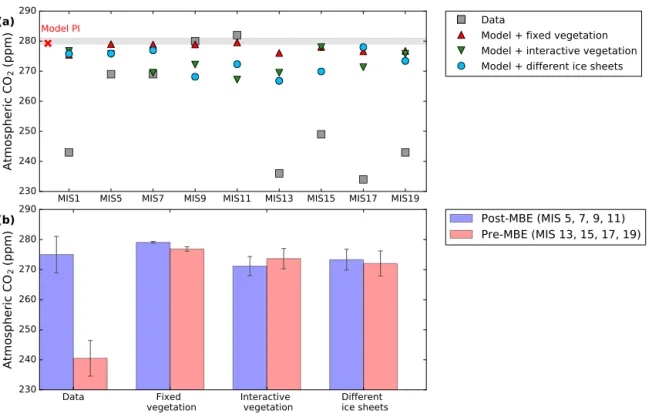
MIS1 MIS5 MIS7 MIS9 MIS11 MIS13 MIS15 MIS17 MIS19 230 240 250 260 270 280 290 A tm o sp h e ri c C O2 ( p p m ) Model PI (a) Data
Model + fixed vegetation Model + interactive vegetation Model + different ice sheets
Data Fixed
vegetation Interactive vegetation ice sheetsDifferent 230 240 250 260 270 280 290 A tm o sp h e ri c C O2 ( p p m ) (b) Post-MBE (MIS 5, 7, 9, 11) Pre-MBE (MIS 13, 15, 17, 19)
Figure 11.(a) CO2concentration (ppm) at the end of the simulations and (b) composite (average) CO2(ppm) in the pre-MBE (MIS 13, 15, 17, 19) and post-MBE (MIS 5, 7, 9, 11) interglacial simulations.
OVC: fixed ice sheets OVIC: different ice sheets
(a) (b)
(c) (d)
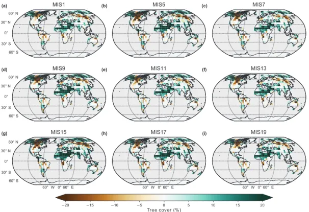
Figure 12.(a, b) Tree cover (%) and (c, d) carbon storage (kg C m−2) difference between pre-MBE (MIS 13, 15, 17, 19) and post-MBE (MIS 5, 7, 9, 11) interglacial simulations for (a, c) the OVC series with interactive vegetation and fixed ice sheets and (b, d) the OVIC series with interactive vegetation and different ice sheets. Qualitative indication of tree cover change from data is indicated with dots: blue indicates a reduction of tree cover on average during pre-MBE interglacials compared to post-MBE interglacials, and red indicates an increase.
American ice sheet is more extended in the pre-MBE inter-glacials compared to the post-MBE interinter-glacials (Fig. 13).
The change of ice sheet extent has a large regional impact on vegetation cover, which is reduced where the ice sheet extends more. On average, it results in a reduction of
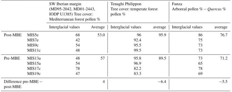
vege-Table 4.Tree cover (%) reconstructed from pollen data at three sites. SW Iberian margin: MIS 5 (MD95-2042, Sanchez Goñi et al., 1999), MIS 7 (MD01-2443; Roucoux et al., 2006), MIS 9, 13, 15, 17 (IODP 1385, unpublished data), MIS 11 (U1385, Oliveira et al., 2016), MIS 19 (U1385, Sanchez Goñi et al., 2016); Tenaghi Philippon, Greece (Past Interglacials Working Group of PAGES, 2016); and Funza, Colombia (Past Interglacials Working Group of PAGES, 2016).
SW Iberian margin (MD95-2042, MD01-2443, IODP U1385) Tree cover: Mediterranean forest pollen %
Tenaghi Philippon
Tree cover: temperate forest pollen %
Funza
Arboreal pollen % − Quercus %
Interglacial values Average Interglacial values average Interglacial values average
Post-MBE MIS5e 68 53.0 96 95.9 86 76.7 MIS7e 42 92.4 75 MIS9c 54 95.5 73 MIS11c 48 99.5 73 Pre-MBE MIS13a 48 57 95.8 89.5 73 71.2 MIS15a 54 96.9 65 MIS17c 78 82.2 78 MIS19c 47 83.3 69 Difference pre-MBE − post-MBE 4 −6.4 −5.5 800 400 0 400 800 Elevation (m)
Figure 13.Ice sheet elevation difference (m) between the average of the pre-MBE (MIS 13, 15, 17, 19) and post-MBE (MIS 5, 7, 9, 11) interglacial simulations.
tation in North America in the pre-MBE interglacials, when the ice sheet is more extended, compared to the post-MBE interglacials (Fig. 12b and d).
The increase in ice sheet extent and diminution of vege-tation cover for pre-MBE simulations has two main impacts for the carbon cycle: (i) it diminishes the terrestrial biosphere carbon storage, increasing atmospheric CO2 and (ii) it also
cools global climate due to the high ice albedo. The SST also
decreases by 0.32◦C on the global scale. Sea surface tem-perature changes are especially pronounced in polar zones, with a drop of 0.49◦C in the North Atlantic and 0.47◦C in the Southern Ocean (Fig. 14 compared to Fig. 4b). Conse-quently, the ocean carbon storage increases, which lowers at-mospheric CO2. This second effect dominates and the overall
result is lower atmospheric CO2 concentration in pre-MBE
simulations compared to post-MBE simulations (Fig. 11). As for the other processes analysed, they only modifies at-mospheric CO2by a few parts per million, though
correct-ing back (compared to OVC simulations) the difference pre-MBE minus post-pre-MBE towards the observations. Neverthe-less, the correlation between simulated and measured CO2
(accounting for MIS1) is very small (−0.08) and not sig-nificant (p = 0.83). The magnitude of the changes of atmo-spheric CO2among the different interglacials is once again
largely underestimated as compared to observations. Accounting for different ice sheets in the OVIC series seems to improve the model–data comparison in southern Europe for tree cover (Fig. 12b) where the data are at the limit between regions of more tree coverage and less tree coverage in the model. This highlights the role of ice sheet extent in setting the vegetation pattern. Nevertheless, the uncertainty in ice sheet distribution is very large and the model-based re-construction might not be accurate. For example, the lack of ice-rafted debris from North America before MIS16 and the presence of ice-rafted debris from Europe indicate that the ice sheet over Europe (Hoddell et al., 2008) could have been more extended and the Laurentide ice sheets in North Amer-ica were not. In addition, the model-based reconstruction that we used shows relatively small changes of sea level equiva-lent between interglacials. Data reconstructions seem to
indi-90° S 60° S 30° S 0° 30° N 60° N 90° N 160° W 120° W 80° W 40°W 0° 40° E 80° E 120° E 160° E 0.6 0.4 0.2 0.0 0.2 0.4 0.6
Sea surface temperature (oC)
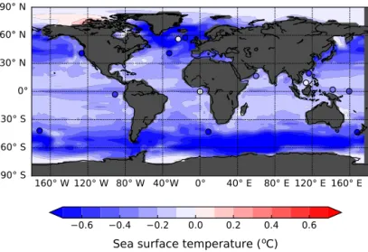
Figure 14.Annual sea surface temperature difference (◦C) between the average of the pre-MBE (MIS 13, 15, 17, 19) and post-MBE (MIS 5, 7, 9, 11) interglacials with interactive vegetation and different ice sheets (OVIC). The vertical black line indicates the limit between the Southern Ocean south of 32◦S and the Atlantic Ocean north of 32◦S. The dots are SST data differences based on the Past Interglacials Working Group of PAGES (2016) (Table 3).
cate possible larger differences between interglacials (Spratt and Lisiecki, 2016), whose effect on the size of the land sur-face and the carbon cycle remains to be tested. Sensitivity experiments with prescribed idealised ice sheets designed to be very different would help to evaluate their impact.
4 Conclusions
Using a fully coupled climate model of intermediate com-plexity including an interactive carbon cycle, we have shown that the difference between pre-MBE and post-MBE can-not be explained by the simulated changes in ocean and vegetation induced by orbital and greenhouse gases forc-ing. While the oceanic response alone is in qualitative agree-ment with data (sign of the changes, correlation between each interglacial), it largely underestimates the amplitude of the changes. Past work suggested that either a vigorous AABW (Yin, 2013) or weak Atlantic thermohaline circulation (Köh-ler and Fischer, 2006) during pre-MBE interglacials could in-crease the oceanic carbon storage and explain the lower CO2
than during post-MBE interglacials. Other studies for differ-ent background climates have shown opposite results with respect to the effect of ocean circulation on carbon storage. A weaker Atlantic meridional oceanic circulation could ei-ther result in more ocean carbon storage with a pre-industrial climate (Obata, 2007; Menviel et al., 2008; Bozbiyik et al., 2011) or glacial climate (Menviel et al., 2008), or it could yield less ocean carbon storage with a pre-industrial climate (Marchal et al., 1998; Swingedouw et al., 2007b; Bouttes et al., 2012) or a glacial climate (Schmittner and Galbraith, 2008; Bouttes et al., 2012; Schmittner and Lund, 2015). Menviel et al. (2014) showed that on top of changes in North Atlantic Deep Water formation, modifications of AABW and
North Pacific Deep Water (NPDW) formations could results in different oceanic carbon storage. Data indicate that the modern reduction of carbon uptake in the North Atlantic is due to a reduction in the overturning circulation (Perez et al., 2013). Because the atmospheric CO2 change that we
sim-ulate has a low magnitude of only a few parts per million, it is not yet possible to infer whether stronger or weaker overturning during pre-MBE interglacials could have signif-icantly lowered atmospheric CO2.
Furthermore, accounting for the vegetation response com-plicates the simulated response and entirely removes the qualitative agreement. The vegetation response depends on ice sheet extent, and accounting for ice sheet variations lim-its the disagreement. Comparison of simulated vegetation changes with available pollen data indicates partial agree-ment, underlying the need to improve vegetation simula-tions and increase the data coverage to more precisely con-strain the change of vegetation cover. The vegetation model in iLOVECLIM only simulates grass and trees; to better eval-uate the different vegetation responses to orbital and CO2
forcings it would be useful to use a more complex terrestrial biosphere model.
We argue that additional processes need to be accounted for or should be better represented in climate models to ex-plain the observations. It is possible that either many different processes, some of them not included in the present model, lead to the observed atmospheric CO2concentration or that
just a first-order process is misrepresented or not included. In particular, the storage of carbon in frozen soils (permafrost) should be included in future modelling work. Response of the Southern Ocean, the widest oceanic region with large air– sea fluxes of CO2, is also a good candidate, given the known
repre-sentation of the key element of its dynamics (eddies, kata-batic winds, AABW formation, brines, etc.). The impact of ventilation changes could be tested by artificially modifying the buoyancy forcing in the areas of bottom water formation. The use of higher-resolution models in this region could help to better evaluate its response to different interglacial condi-tions.
Data availability. The model output data is provided in the Sup-plement.
The Supplement related to this article is available online at https://doi.org/10.5194/cp-14-239-2018-supplement.
Competing interests. The authors declare that they have no con-flict of interest.
Acknowledgements. We are grateful to the two anonymous reviewers for their useful comments. The research leading to these results has received funding from the European Union’s Horizon 2020 research and innovation programme under grant agreement no. 656625, project “CHOCOLATE”. We also acknowledge Warm-Clim, a LEFE-INSU IMAGO project. All the simulations have been performed on the Avakas computer cluster from the Mésocentre de Calcul Intensif Aquitain (MCIA). We thank Vincent Marieu for his assistance in setting up the model on this supercomputer. Discussions with Anne-Sophie Kremer and Thibaut Caley were useful to develop this paper and are acknowledged.
Edited by: Arne Winguth
Reviewed by: two anonymous referees
References
Bereiter, B., Eggleston, S., Schmitt, J., Nehrbass-Ahles, C., Stocker, T. F., Fischer, H., Kipfstuhl, S., and Chappellaz, J.: Revision of the EPICA Dome C CO2 record from 800 to 600 kyr before present, Geophys. Res. Lett., 42, 542–549, https://doi.org/10.1002/2014GL061957, 2015.
Berger A.: Long-term variations of daily insolation and quaternary climatic changes, J. Atmos. Sci., 35, 2362–2367, 1978. Bouttes, N., Roche, D. M., and Paillard, D.: Systematic study of the
impact of fresh water fluxes on the glacial carbon cycle, Clim. Past, 8, 589–607, https://doi.org/10.5194/cp-8-589-2012, 2012. Bouttes, N., Roche, D. M., Mariotti, V., and Bopp, L.: Including
an ocean carbon cycle model into iLOVECLIM (v1.0), Geosci. Model Dev., 8, 1563–1576, https://doi.org/10.5194/gmd-8-1563-2015, 2015.
Bozbiyik, A., Steinacher, M., Joos, F., Stocker, T. F., and Men-viel, L.: Fingerprints of changes in the terrestrial carbon cycle in response to large reorganizations in ocean circulation, Clim. Past, 7, 319–338, https://doi.org/10.5194/cp-7-319-2011, 2011.
Brovkin, V., Ganopolski, A., and Svirezhev, Y.: A continuous climate-vegetation classification for use in climate-biosphere studies, Ecol. Model., 101, 251–261, 1997.
Brovkin, V., Bendtsen, J., Claussen, M., Ganopolski, A., Ku-batzki, C., Petoukhov, V., and Andreev, A.: Carbon cycle, veg-etation and climate dynamics in the Holocene: experiments with the CLIMBER-2 model, Global Biogeochem. Cyc., 16, 1139, https://doi.org/10.1029/2001GB001662, 2002.
Calov, R., Ganopolski, A., Claussen, M., Petoukhov, V., and Greve. R.: Transient simulation of the last glacial inception, Part I: Glacial inception as a bifurcation of the climate system, Clim. Dynam., 24, 545–561, https://doi.org/10.1007/s00382-005-0007-6, 2005.
Crichton, K. A., Bouttes, N., Roche, D. M., Chappellaz, J., and Krinner, G.: Permafrost carbon as a missing link to explain CO2 changes during the last deglaciation, Nat. Geosci., 9, 683–686, https://doi.org/10.1038/ngeo2793, 2016.
Fischer, H., Schmitt, J., Lüthi, D., Stocker, T. F., Tschumi, T., Parekh, P., Joos, F., Köhler, P., Völker, C., Gersonde, R., Bar-bante, C., Le Floch, M., Raynaud, D., and Wolff, E.: The role of Southern Ocean processes on orbital and millennial CO2 variations – a synthesis, Quaternary Sci. Rev., 29, 193–205, https://doi.org/10.1016/j.quascirev.2009.06.007, 2010.
Ganopolski, A. and Calov, R.: The role of orbital forcing, carbon dioxide and regolith in 100 kyr glacial cycles, Clim. Past, 7, 1415–1425, https://doi.org/10.5194/cp-7-1415-2011, 2011. Ganopolski, A., Petoukhov, V., Rahmstorf, S., Brovkin, V.,
Claussen, M., Eliseev, A., and Kubatzki, C.: CLIMBER-2: a cli-mate system model of intermediate complexity, Part II: Model sensitivity, Clim. Dynam., 17, 735–751, 2001.
Goosse, H., Brovkin, V., Fichefet, T., Haarsma, R., Huybrechts, P., Jongma, J., Mouchet, A., Selten, F., Barriat, P.-Y., Campin, J.-M., Deleersnijder, E., Driesschaert, E., Goelzer, H., Janssens, I., Loutre, M.-F., Morales Maqueda, M. A., Opsteegh, T., Math-ieu, P.-P., Munhoven, G., Pettersson, E. J., Renssen, H., Roche, D. M., Schaeffer, M., Tartinville, B., Timmermann, A., and Weber, S. L.: Description of the Earth system model of intermediate complexity LOVECLIM version 1.2, Geosci. Model Dev., 3, 603–633, https://doi.org/10.5194/gmd-3-603-2010, 2010.
Greve, R.: A continuum-mechanical formulation for shallow poly-thermal ice sheets, Philos. T. R. Soc. Lond., 355, 921–974, 1997. Heuzé, C., Heywood, K. J., Stevens, D. P., and Rid-ley, J. K.: Southern Ocean bottom water characteristics in CMIP5 models, Geophys. Res. Lett., 40, 1409–1414, https://doi.org/10.1002/grl.50287, 2013.
Hodell, D. A., Channell, J. E. T., Curtis, J. H., Romero, O. E., and Röhl, U.: Onset of “Hudson Strait” Heinrich events in the eastern North Atlantic at the end of the middle Pleis-tocene transition (∼ 640 ka)?, Paleoceanography, 23, PA4218, https://doi.org/10.1029/2008PA001591, 2008.
Köhler, P. and Fischer, H.: Simulating low frequency changes in atmospheric CO2during the last 740 000 years, Clim. Past, 2, 57–78, https://doi.org/10.5194/cp-2-57-2006, 2006.
Lang, N. and Wolff, E. W.: Interglacial and glacial variability from the last 800 ka in marine, ice and terrestrial archives, Clim. Past, 7, 361–380, https://doi.org/10.5194/cp-7-361-2011, 2011.
Lisiecki, L. E. and Raymo, M. E.: A Pliocene–Pleistocene stack of 57 globally distributed benthic δ18O records, Paleoceanography, 20, PA1003, https://doi.org/10.1029/2004PA001071, 2005. Lüthi, D., Le Floch, M., Bereiter, B., Blunier, T., Barnola, J.-M.,
Siegenthaler, U., Raynaud, D., Jouzel, J., Fischer, H., Kawa-mura, K., and Stocker, T. F.: High-resolution carbon dioxide con-centration record 650,000–800,000 years before present, Nature, 453, 379–382, https://doi.org/10.1038/nature06949, 2008. Marchal, O., Stocker, T. F., and Joos, F.: Impact of oceanic
reor-ganizations on the ocean carbon cycle and atmospheric carbon dioxide content, Paleoceanography, 13, 225–244, 1998. Menviel, L., Timmermann, A., Mouchet, A., and Timm, O.:
Meridional reorganizations of marine and terrestrial produc-tivity during Heinrich events, Paleoceanography, 23, PA1203, https://doi.org/10.1029/2007PA001445, 2008.
Menviel, L., England, M. H., Meissner, K., Mouchet, A., and Yu, J.: Atlantic–Pacific seesaw and its role in outgassing CO2 during Heinrich events, Paleoceanography, 29, 58–70, https://doi.org/10.1002/2013PA002542, 2014.
Obata, A.: Climate–carbon cycle model response to freshwater discharge into the North Atlantic, J. Climate, 20, 5962–5976, https://doi.org/10.1175/2007JCLI1808.1, 2007.
Oliveira, D., Desprat, S., Rodrigues, T., Naughton, F., Hodell, D., Trigo, R., Rufino, M., Lopes, C., Abrantes, F., and Sánchez Goñi, M. F.: The complexity of millennial-scale variability in southwestern Europe during MIS 11, Quaternary Res., 86, 373– 387, https://doi.org/10.1016/j.yqres.2016.09.002, 2016. Past Interglacials Working Group of PAGES: Interglacials
of the last 800,000 years, Rev. Geophys., 54, 162–219, https://doi.org/10.1002/2015RG000482, 2016.
Pérez, F. F., Mercier, H., Vázquez-Rodríguez, M., Lherminier, P., Velo, A., Pardo, P. C., Rosón, G., and Ríos, A. F.: At-lantic Ocean CO2 uptake reduced by weakening of the meridional overturning circulation, Nat. Geosci., 6, 146–152, https://doi.org/10.1038/NGEO1680, 2013.
Petoukhov, V., Ganopolski, A., Brovkin, V., Claussen, M., Eliseev, A., Kubatzki, C., and Rahmstorf, S.: CLIMBER-2: a cli-mate system model of intermediate complexity, Part I: Model de-scription and performance for present climate, Clim. Dynam., 16, 1– 17, 2000.
Roucoux, K. H., Tzedakis, P. C., de Abreu, L., and Shack-leton, N. J.: Climate and vegetation changes 180,000 to 345,000 years ago recorded in a deep-sea core off Portugal, Earth Planet. Sc. Lett., 249, 307–325, 2006.
Sanchez-Goni, M. F., Eynaud, F., Turon, J. L., and Shackleton, N. J.: High resolution palynological record off the Iberian margin: di-rect land–sea correlation for the Last Interglacial complex, Earth Planet. Sc. Lett., 171, 123–137, 1999.
Sánchez Goñi, M. F., Rodrigues, T., Hodell, D. A., Polanco-Martinez, J. M., Alonso-Garcia, M., Hernandez-Almeida, I., De-sprat, S., and Ferretti, P.: Tropically-driven climate shifts in southwestern Europe during MIS 19, a low excentricity inter-glacial, Earth Planet. Sc. Lett., 448, 81–93, 2016.
Schmittner, A. and Galbraith, E. D.: Glacial greenhouse-gas fluc-tuations controlled by ocean circulation changes, Nature, 456, 373–376, https://doi.org/10.1038/nature07531, 2008.
Schmittner, A. and Lund, D. C.: Early deglacial Atlantic over-turning decline and its role in atmospheric CO2 rise in-ferred from carbon isotopes (δ13C), Clim. Past, 11, 135–152, https://doi.org/10.5194/cp-11-135-2015, 2015.
Spratt, R. M. and Lisiecki, L. E.: A Late Pleistocene sea level stack, Clim. Past, 12, 1079–1092, https://doi.org/10.5194/cp-12-1079-2016, 2016.
Swingedouw, D., Braconnot, P., Delecluse, P., Guilyardi, E., and Marti, O.: Quantifying the AMOC feedbacks during a 2 × CO2 stabilization experiment with land-ice melting, Clim. Dynam., 29, 521–534, 2007a.
Swingedouw, D., Bopp, L., Matras, A., and Braconnot, P.: Effect of land-ice melting and associated changes in the AMOC result in little overall impact on oceanic CO2uptake, Geophys. Res. Lett., 34, L23706, https://doi.org/10.1029/2007GL031990, 2007b. Yin, Q.: Insolation-induced mid-Brunhes transition in Southern
Ocean ventilation and deep-ocean temperature, Nature, 494, 222–225, https://doi.org/10.1038/nature11790, 2013.
Yin, Q. Z. and Berger, A.: Insolation and CO2contribution to the interglacial climate before and after the Mid-Brunhes Event, Nat. Geosci., 3, 243–246, https://doi.org/10.1038/ngeo771, 2010. Yin, Q. Z. and Berger, A.: Individual contribution of insolation and
CO2to the interglacial climates of the past 800,000 years, Clim. Dynam., 38, 709–724, 2012.