D
uring the past two centuries, human activities have greatly modified the exchange of carbon and nutrients between the land, atmosphere, freshwater bodies, coastal zones and the open ocean1–9. Together, land-use changes, soil erosion, liming, fertilizer and pesticide application, sewage-water production, dam-ming of water courses, water withdrawal and human-induced cli-matic change have modified the delivery of these elements through the aquatic continuum that connects soil water to the open ocean through rivers, streams, lakes, reservoirs, estuaries and coastal zones, with major impacts on global biogeochemical cycles10–14. Carbon is transferred through the aquatic continuum laterally across ecosys-tems and regional geographic boundaries, and exchanged vertically with the atmosphere, often as greenhouse gases (Box 1).Although the importance of the aquatic continuum from land to ocean in terms of its impact on lateral C fluxes has been known for more than two decades15, the magnitude of its anthropogenic perturbation has only recently become apparent8,12,16–18. The lateral transport of C from land to sea has long been regarded as a nat-ural loop in the global C cycle unaffected by anthropogenic per-turbations. Thus, this flux is at present neglected in assessments of the budget of anthropogenic CO2 reported, for instance, by the Intergovernmental Panel on Climate Change (IPCC) or the Global Carbon Project19–23. Quantifying lateral C fluxes between land and ocean and their implications for CO2 exchange with the atmosphere is important to further our understanding of the mechanisms driv-ing the natural C cycle along the aquatic continuum24,25, as well as for closing the C budget of the ongoing anthropogenic perturbation.
Data related to the C cycle in the aquatic continuum from land to ocean are too sparse to provide a global coverage, with insuf-ficient water sampling, poorly constrained hydrology and surface area extent of various ecosystems, and few direct pCO2 and other carbon-relevant measurements26,27. Global box models have been used to explore the magnitude of these fluxes and their anthropo-genic perturbations, but the processes remain highly parameter-ized7. The current generation of three-dimensional Earth system models includes the coupling between the C cycle and the physical
Anthropogenic perturbation of the carbon fluxes
from land to ocean
Pierre Regnier et al.
†A substantial amount of the atmospheric carbon taken up on land through photosynthesis and chemical weathering is transported laterally along the aquatic continuum from upland terrestrial ecosystems to the ocean. So far, global carbon budget estimates have implicitly assumed that the transformation and lateral transport of carbon along this aquatic continuum has remained unchanged since pre-industrial times. A synthesis of published work reveals the magnitude of present-day lateral carbon fluxes from land to ocean, and the extent to which human activities have altered these fluxes. We show that anthropogenic perturbation may have increased the flux of carbon to inland waters by as much as 1.0 Pg C yr-1 since pre-industrial times, mainly owing to enhanced carbon export from soils. Most of this additional carbon input to upstream rivers is either emitted back to the atmosphere as carbon dioxide (~0.4 Pg C yr-1) or sequestered in sediments (~0.5 Pg C yr-1) along the continuum of freshwater bodies, estuaries and coastal waters, leaving only a perturbation carbon input of ~0.1 Pg C yr-1 to the open ocean. According to our analysis, terrestrial ecosystems store ~0.9 Pg C yr-1 at present, which is in agreement with results from forest inventories but significantly differs from the figure of 1.5 Pg C yr-1 previously estimated when ignoring changes in lateral carbon fluxes. We suggest that carbon fluxes along the land–ocean aquatic continuum need to be included in global carbon dioxide budgets.
climate system, but ignores lateral flows of C (and nutrients) alto-gether28. Major challenges in the study of C in the aquatic contin-uum include the disentangling of the anthropogenic perturbations from the natural transfers, identifying the drivers responsible for the ongoing changes and, ultimately, forecasting their future evo-lution, for example, by incorporating these processes in Earth sys-tem models. Resolving these issues is not only necessary to refine the allocation of greenhouse-gas fluxes at the global and regional scale, but also to establish policy-relevant regional budgets and mitigation strategies29.
The term ‘boundless carbon cycle’ was introduced to designate the present-day lateral and vertical C fluxes to and from inland waters only17. Here, we extend this concept to all components of the global C cycle that are connected by the land–ocean aquatic con-tinuum (Box 1) and discuss possible changes relative to the natu-ral C cycle by providing new separate estimates for the present day and the anthropogenic perturbation. This distinction is important because, in some instances, bulk fluxes have been compared with perturbation fluxes, such as the net land C sink of anthropogenic CO2, which may cause confusion17,30. Here we deal with the total C fluxes, but do not systematically distinguish between inorganic and organic, as this is still poorly known at the global scale for several of the components of the land–ocean continuum. However, we do highlight the exact chemical composition where it is sufficiently well constrained. Supplementary Table S1 is a compilation of the major flux estimates from the literature and estimated in this paper with a measure of confidence involving transfer of C from one global domain to another. A brief justification of our proposed estimate for each of these fluxes is also provided.
Contemporary estimates of lateral carbon fluxes
In this section, we derive contemporary estimates of the carbon fluxes along the continuum of the spectrum of land–ocean aquatic systems. We first look at the C transports involving inland waters and then consider their links to C flows through estuaries and the coastal ocean and beyond.
Inland waters. The present-day bulk C input (natural plus anthro-pogenic) to freshwaters was recently estimated at 2.7–2.9 Pg C yr–1, based on upscaling of local C budgets17,26. This input is composed of four fluxes. The first and largest one is soil-derived C that is released to inland waters, mainly in organic form (particulate and dissolved), but also as free dissolved CO2 from soil respiration31 (F1 in Fig. 1a and Table 1). The flux is evaluated at 1.9 Pg C yr–1, by subtracting, from a total median estimate of 2.8 Pg C yr–1, the smaller contribu-tions from the other three fluxes: chemical weathering (F2), sewage (F4) and net C fixation (F5). The soil-derived C flux is part of the terrestrial ecosystem C cycle (Box 1) and represents about 5% of soil heterotrophic respiration (FT7). Current soil respiration estimates neglect the C released to inland waters. A downward revision of the estimate of soil heterotrophic respiration to account for the soil C channelled to inland freshwater systems would nevertheless remain within the uncertainty of this flux32.
The second flux involves the chemical weathering of continental surfaces (carbonate and silicate rocks). It is part of the inorganic
(often called ‘geological’) C cycle (Box 1) and causes an additional ~0.5 Pg C yr–1 input to upstream rivers33–37 (F
2). About two-thirds of this C flux is due to removal of atmospheric CO2 in weathering reactions (F3) and the remaining fraction originates from cal weathering of C contained in rocks. The pathway for chemi-cal weathering is nevertheless largely indirect with most of the CO2 removed from the atmosphere being soil CO2, having passed through photosynthetic fixation. Weathering releases C to the aquatic continuum in the form of dissolved inorganic C, mainly bicarbonate, given that the average pH is in the range of 6–8 for freshwater aquatic systems38. In contrast to soil-derived organic C, it is assumed that C derived from rock weathering will not degas to the atmosphere during its transfer through inland waters39.
The third flux represents the C dissolved in sewage water origi-nating from biomass consumption by humans and domestic ani-mals (F4), which releases an additional ~0.1 Pg C yr–1 as an input to freshwaters40,41. The fourth flux involves photosynthetic C fixation within inland waters, potentially high on an areal basis16. A sub-stantial fraction of this C is returned to the atmosphere owing to decomposition within inland waters42, but a percentage remains for export and burial43,44, and priming of terrestrial organic matter decomposition45. Thus, although aquatic systems can emit CO
2 to the atmosphere, they still can be autotrophic46. We estimate with low confidence that 20% of the organic C buried and exported from inland waters (see below for estimations) is autochthonous (F5).
Physical erosion of particulate inorganic C (~0.2 Pg C yr–1) and of organic C that is resistant to mineralization (~0.1 Pg C yr–1) represents another C source to the aquatic continuum47,48 (F
R). Although the fate of this physically eroded C is difficult to trace, it is likely to be refractory at the centennial timescale49 and is most likely channelled through inland waters and estuaries to the open ocean without significant exchange with the atmosphere. It is thus treated separately in Fig. 1a.
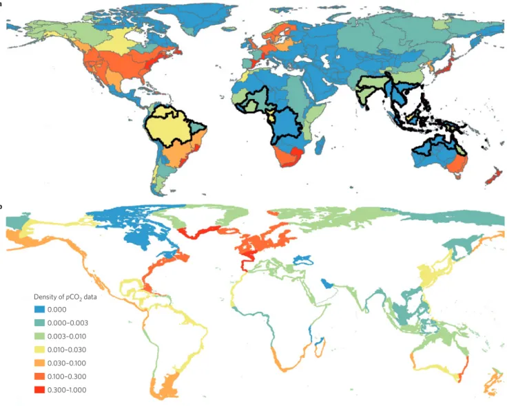
During the transport of C from soils to the coastal ocean, a fraction of the lateral flux that transits through inland waters is emitted to the atmosphere, mainly as CO2 (F7). CH4 is also emitted from lakes and some rivers (F6), but this flux represents a small fraction of the laterally transported C flux30. Data-driven estimates of the water-to-atmosphere CO2 efflux have been obtained for individual components of the inland freshwater continuum16,17,50. This efflux is sustained by CO2 originating from root and soil respiration, aquatic decomposition of dissolved and particulate organic matter, and decomposition of organic C from sewage, as detailed above. Furthermore, the addition of C from fringing and riparian wetlands, counted as soil C input to freshwaters in Fig. 1a, may also contribute significantly to freshwater CO2 outgassing51. Approximately 12,000 sampling locations of the inorganic C cycle are now reported in inland water databases (Fig. 2a). Calculation of pCO2 from alkalinity and pH indicates that 96% of inland waters are oversaturated with respect to CO2 relative to its atmos-pheric concentration, while 82% have a concentration of at least twice that of the atmosphere (Global River Chemistry Database (GloRiCh), unpublished data; ref. 52).
Numerous measurements of the freshwater CO2 efflux are avail-able for some regions of the globe, such as the Rhine catchment, Scandinavia and the conterminous United States39,42,51–53. However, lack of direct CO2 flux measurements, incomplete spatial coverage of pCO2 sampling locations coupled with the difficulty in determin-ing the surface area of inland waters, and scaldetermin-ing the gas-transfer velocity in freshwaters, causes large uncertainties and prevents us from obtaining robust global-scale estimates (Fig. 2a). In particular, many rivers and lakes that contribute a significant fraction to the aquatic C flux remain poorly surveyed in terms of pCO2 (GloRiCh, unpublished data). These include the rivers of Southeast Asia, tropi-cal Africa and the Ganges and, to a lesser extent, the waters of the Amazon Basin54,55, which carry disproportionally high organic
The land–ocean aquatic continuum. This can be represented
as a succession of chemically and physically active biogeochem-ical systems, all connected through the continuous water film that starts in upland soils and ends in the open ocean. Carbon is transferred along this continuum. These systems are often referred to as filters, because carbon is not only transferred, but also processed biogeochemically and sequestered in sediments or exchanged with the overlying atmosphere as greenhouse gases (Fig. 1a).
The pre-industrial land–ocean loops. Lateral carbon transfer
through the aquatic continuum was already active under pre-industrial conditions and the boundless carbon cycle consists of two loops. The organic carbon loop starts with the lateral leakage of some of the organic carbon that is fixed into the terrestrial biosphere by photosynthesis. This carbon is then transferred horizontally through aquatic channels down to the coastal and open ocean where C is returned to the atmosphere as CO2. The inorganic loop is driven by the land-based weath-ering of silicate and carbonate rocks that consumes atmos-pheric CO2, and the subsequent transport of the weathering products of cations, anions and dissolved inorganic carbon to the ocean, where part of the CO2 is returned to the atmosphere through ocean carbonate sediment formation (a process that increases pCO2 in seawater). The other part is returned by vol-canism. Both loops are generally assumed to have been in a quasi-steady-state initial condition in pre-industrial times, that is, they were globally balanced at the millennial timescale.
Anthropogenic perturbation of the lateral carbon fluxes.
Human perturbations to the lateral carbon fluxes have moved the boundless carbon cycle away from this global balance, causing imbalances in the fluxes and stocks, such as the C inputs from soils to inland water systems, the strength of the air–water CO2 exchange fluxes, the C storage reservoirs and, thus, the chain of lateral C fluxes through the successive filters. Because the reconstruction of lateral carbon fluxes entails large uncertainties, we only attempt quantification for pre-industrial and present-day (past decade) conditions. We thus regard the change in the fluxes and stocks since the pre-industrial period as the anthropogenic perturbation, and treat the average pre-industrial conditions as the natural contribution.
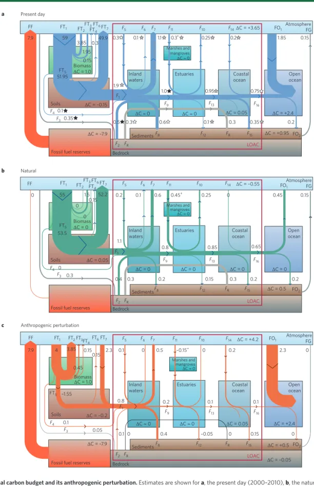
FF 1.95 0.15 0 0.45 0 0.1 0.2 0.25 Inland waters Inland waters Coastal ocean Coastal ocean Open ocean Open ocean Estuaries Estuaries Marshes and mangroves ∆C ≈ 0 Marshes and mangroves ∆C ≈ 0 ∆C ≈ 0 ∆C ≈ 0 0.45 0.15 Atmosphere FG 0.6 0.45+ 0 0 55 53.5 Soils Soils FF FT1 FT5 FT5 FT2 FT3 FT4 F4 F4 F3 0.1 0.05 F3 0 1.1 0.8 0.85 0.65 0.3 0.4 0.3 0.2 7.9 3.85 0.15 1.5 0.1552.2 0.15 –0.15 + 2.3 0.1 0 4 0 0.2 0.1 0.1 0.2 0.8 0.1 0 0.4 –0.05 0 0.15 0 –1.55 2.3 0 0.5 0.2 LOAC LOAC 0.2 0.3 0.15 FT6FT7 F 5 F6 F9 F1 F13 F16 F7 F11 F10 F14 FO1 Atmosphere FG FF FT1 F1 FT2FT3FT 4FT6FT7 F5 F6 F7 F11 F9 F13 F16 F10 F14 FO1 FO2 F15 FR F12 F8 F2 FR F2 FR Bedrock Bedrock Sediments Fossil fuel reserves
Fossil fuel reserves Biomass ∆C = 1.0 Biomass ∆C = 0 Biomass ∆C = 1.0 ∆C = –0.15 ∆C ≈ 0 ∆C ≈ 0 ∆C = 0.05 ∆C = +2.4 ∆C = +0.95 ∆C = +3.65 ∆C = –7.9 59 0.1 0.35 0.5 0.3 0.6 0.1 0.3 0.35 0.2 Soils 3.85 0.349.9 7.9 51.95 0.3 1.9 1.0 0.95 0.75 Inland waters Estuaries Marshes and mangroves ∆C ≈ 0 Sediments LOAC Bedrock Fossil fuel reserves
Coastal
ocean Openocean
0.1 1.1 0.3+ 0.25 0.2 1.85 0.15 F1 F9 F8 F2 FR F12 FR F15 FO2 F13 F16 F4 F3 FT5 FT2 FT1 FTFT3FT46FT7 F5 F6 F7 F11 F10 F14 FO1 AtmosphereFG a b c Present day Natural Anthropogenic perturbation ∆C = –0.55 ∆C = 0.5 FO2 F15 FR F12 F8 Sediments ∆C = +0.5 ∆C = –7.9 ∆C = –0.05 ∆C = +4.2 ∆C = 0 ∆C = 0 ∆C = 0 ∆C = 0 ∆C = +2.4 ∆C = 0.05 ∆C = –0.2 ∆C = 0.05
Figure 1 | Global carbon budget and its anthropogenic perturbation. Estimates are shown for a, the present day (2000–2010), b, the natural C cycle
(
~
1750) and c, the anthropogenic perturbation only. All fluxes are in Pg C yr–1, rounded to ±0.05 Pg C yr–1, and refer to total C fluxes (organic and inorganicC). The numbers associated with the arrows are fluxes between reservoirs. Boxed ΔC refers to C accumulation within each reservoir. The red box delineates the succession of lateral C filters along the land–ocean aquatic continuum (LOAC). The + sign indicates that C sequestration from estuaries and adjacent coastal vegetation are merged in the figure. The stars in panel a indicate the confidence interval associated to the flux estimates, based on The
First State of the Carbon Cycle Report99. A black star means 95% certainty that the actual estimate is within 50% of the estimate reported; a grey star means
95% certainty that the actual value is within 100% of the estimate reported; a white star corresponds to an uncertainty greater than 100%. Flux symbols are defined in Table 1.
carbon loads owing to their combination of high terrestrial pro-ductivity, high decomposition rates and high uniform precipitation rates (Fig. 2a). The scarcity of direct pCO2 measurements and lack of knowledge on regional surface area and gas-transfer velocity explain the large uncertainty in the CO2 outgassing from freshwaters8,16,26,51, with a range of 0.6–1.25 Pg C yr–1. The values at the higher end of the spectrum also include the contribution of streams and small lakes, which are typically not considered in flux estimates26. We estimate a most likely value of the CO2 outgassing flux of 1.1 Pg C yr–1 (F7) with a medium-to-low confidence.
The burial rate in freshwater sediments has been estimated to be between ~0.2 and 1.6 Pg C yr–1. The lower estimate refers to lakes, ponds and reservoirs only16,26 (0.2–0.6 Pg C yr–1), whereas the upper one also includes sedimentation in floodplains6,56,57 (0.5– 1.6 Pg C yr–1). The factor of eight between the lower and higher bound estimates of this burial flux highlights the limited obser-vational data available to constrain this term at the global scale. Within this large uncertainty, we adopt with a low confidence a value of 0.6 Pg C yr–1 for the C burial in inland water sediments (F
8). Part of this burial is carbon transported, by erosion processes, from soils to lake sediments and floodplains.
From the mass balance of the C input from soils to fresh waters minus CO2 outgassing and C burial fluxes in inland waters adopted here, the output represents a lateral C flux transported downstream into estuarine systems (F9) of 1.0 Pg C yr–1. Thus our estimate is
close to values based on compilation of field data and the results of the Global Nutrient Export from Watersheds model of carbon and water flows59, although higher values have also been suggested8. A flux of particulate and dissolved organic C, each equivalent to about 0.2 Pg C yr–1, and a flux of dissolved inorganic C of about 0.4 Pg C yr–1 is the conventional partitioning among the different C pools47,58,60,61. If we take into account the uncertainty for each of the individual inland water fluxes (weathering, outgassing, burial and export), the balance also indicates that the soil-derived C flux (F1, 1.9 Pg C yr–1) is certainly not known any better than within ~±1.0 Pg C yr–1.
Estuaries. In our analysis, estuaries (total area of 1.1 x 10⁶ km2) correspond to the boundary between inland aquatic systems and the coastal ocean, represented mainly by the shelves of the world’s oceans62. Recent syntheses of observational data indicate that estuaries emit CO2 to the atmosphere27,63, within the range of 0.25 ± 0.25 Pg C yr–1 (F
10). Field measurements suggest that about 10% of the CO2 outgassing from estuaries is sustained by the input from upstream freshwaters (F9) and 90% by local net heterotro-phy64, with a significant fraction of the required organic C coming from adjacent marsh ecosystems (F11). Although coastal vegetated environments (salt marshes, mangroves, seagrasses, macroal-gae and coral reefs) may export as much as 0.77–3.18 Pg C yr–1 to the coastal ocean65, we use here a more conservative estimate of ~0.3 ± 0.1 Pg C yr–1 for the common estuarine vegetation of man-groves and salt marshes, which is based on an upscaling of a detailed regional budget for the southeastern United States63. Furthermore, to our knowledge, no global estimates exist for C burial in all estuarine sediments, but a long-term burial in mangroves and salt marshes of 0.1 ± 0.05 Pg C yr–1 has been proposed18,66 (F
12). If we combine our upstream river and coastal vegetation inputs with our average estuarine CO2 outgassing estimate to the atmosphere and the first-order estimate for burial of C in estuarine sediments and vegetated ecosystems (F12), we obtain a C delivery from estuaries to the coastal ocean of 0.95 Pg C yr–1 (F
13). This estimate amounts to about one-third of the initial C flux released from soils, rocks and sewage as input to inland freshwater systems.
Coastal ocean and beyond. Materials leaving estuaries transit into the coastal ocean and beyond to the open ocean. Recent synthe-ses of the air–sea CO2 fluxes in coastal waters (total area of 31 x 106 km2)62 suggest that at present between 0.22 and 0.45 Pg C yr–1 are taken up by the coastal ocean67,68. We choose here a lower estimate of 0.2 Pg C yr–1 for the coastal ocean sink of CO
2, based on a recent analysis for the global ocean69 (F
14). This value relies on the observa-tion that, outside the nearshore environments, the net CO2 fluxes in the coastal regions are of similar strengths and directions to those in the adjacent ocean regions, that is, that low-latitude coastal regions tend to be sources of CO2 to the atmosphere, whereas high-latitude regions tend to be sinks67,68. This allows the extrapolation of the open-ocean CO2 exchange values towards the coasts. Although this extrapolation is an oversimplification, the most recent estimate (0.25 Pg C yr–1) based on the upscaling from a few sites with good observational coverage suggests a similar value63. Nevertheless, it is important to recognize that the limited spatial coverage of pCO2 data in the coastal ocean (Fig. 2b) and its heterogeneous nature con-fine the confidence to low-to-medium. Furthermore, the influence of terrestrial C input on air–sea CO2 fluxes extends considerably beyond the limit of the shelf in the discharge plumes of large tropi-cal rivers, such as the Amazon63,70. These plumes should be consid-ered as an integral part of the land–ocean continuum.
Coastal ocean sediments may sequester between 0.2 and 0.5 Pg C yr–1 of organic C and calcium carbonate71,72, although sig-nificantly higher values have been reported73 (F
15). We choose here a central estimate of 0.35 Pg C yr–1, of which a sediment C burial of
Table 1 | Definition of carbon flux symbols used in Fig. 1.
Symbol Flux name
FF Fossil-fuel emissions
FT1 Net primary production of terrestrial ecosystems
FT2 Harvest, cattle and biofuels emissions (CO2)
FT3 Fire emissions (CO2)
FT4 Cattle, landfills and fire emissions (CH4)
FT5 Terrestrial biomass to soil C flux
FT6 Rice paddies and wetland emissions (CH4)
FT7 Soil heterotrophic respiration (CO2)
F1 Total soil C input to inland waters
F2 Inorganic C input to inland waters from weathering
F3 Atmospheric CO2 uptake by bedrock weathering
F4 Organic C inputs to inland waters (sewage)
F5 Photosynthetically fixed C not respired in inland waters
FR Physical erosion of total recalcitrant C
F6 CH4 emissions from inland waters to the atmosphere
F7 CO2 emissions from inland waters to the atmosphere
F8 Total C burial in inland water sediments
F9 Total lateral C flux from inland waters to estuaries
F10 CO2 emissions from estuaries to the atmosphere
F11 CO2 uptake from marsh ecosystems and subsequent organic C
input to estuaries
F12 Total C burial in estuarine sediments and coastal vegetated
ecosystems
F13 Total lateral C flux from estuaries to the coastal ocean
F14 Atmospheric CO2 uptake by coastal waters
F15 Total C burial in coastal ocean sediments
F16 Total C export from the coastal to the open ocean
FO1 Air–sea CO2 flux in the open ocean
FO2 Total C burial in open ocean sediments
FG Geological fluxes (volcanism, metamorphism and oxidation of fossil organic C)
0.05–0.1 Pg C yr–1 is attributed solely to the seagrass meadows of shallow coastal seas18. In addition, the most probable repository for much of the recalcitrant terrestrial C related to physical weather-ing (FR) is likely to be in coastal sediment C pools74,75. Furthermore, the net pumping of anthropogenic CO2 from the atmosphere into coastal waters may increase the dissolved inorganic carbon stor-age in the water column76, by about 0.05 Pg C yr–1. Because of data paucity, a direct global estimate of lateral C fluxes at the bound-ary between the coastal and open ocean, delineated by the shelf break62, is not at present achievable solely through observational means12,70,77. Thus, based on mass-balance calculations using the above flux estimates, we propose with a low confidence that the net inorganic and organic C export from the coastal ocean to the open ocean is ~0.75 Pg C yr–1 (F
16) as shown in Fig. 1a.
Anthropogenic perturbation of lateral carbon fluxes
As with the contemporary lateral C fluxes, we now trace sequentially
the route of the perturbed C fluxes through the global system of inland waters to estuaries to coastal waters and beyond.
Inland waters. Reconstructions of the historical evolution (pre-industrial, around the year 1750, to present) of the global aquatic C cycle and its fluxes have so far relied primarily on globally aver-aged box models7,74. Increasing concentrations of atmospheric CO
2, land-use changes, nitrogen and phosphorus fertilizer application, C, nitrogen and phosphorus sewage discharge and global surface temperature change drive these highly parameterized models. Model simulations suggest that the transport of riverine C (F9) has increased by about 20% since 1750, from ~0.75 Pg C yr–1 in 1750 to 0.9–0.95 Pg C yr–1 at present. The existence of such an enhanced riv-erine delivery of C is supported by the available literature data3,8,47,78, and has been attributed to deforestation and more intensive culti-vation practices that have increased soil degradation and erosion. This leads to an increase in the export of organic and inorganic C
a b 0.000 0.000–0.003 0.003–0.010 0.010–0.030 0.030–0.100 0.100–0.300 0.300–1.000 Density of pCO2 data
Figure 2 | Density of pCO2 data for the continuum of land–ocean aquatic systems. pCO2 values are shown for a, inland waters (Global River Chemistry
database) and b, continental shelf seas (Surface Ocean Carbon Atlas database). The index reports the data density with respect to spatial coverage (using
a 0.5° resolution) and seasonality. Inland waters are represented by 150 meta-watersheds100, and coastal waters by 45 continental shelf segments62.
The surface area of inland waters within each segment is available at www.biogeomod.net/geomap. The index is calculated following the equation I = (∑n
i=1 ci )/(n×12) where I is the index itself, n is the number of 0.5° grid cells and ci is the count corresponding to the number of months for which at least one pCO2 value exists within the grid cell i. A value of 0 indicates a complete absence of data and a value of 1 indicates the presence of at least one
pCO2 value every month in each of the grid cells of the considered area. The black lines in a represent the limits of hotspot areas for CO2 evasion to the
to aquatic systems. For example, erosion of particulate organic C in the range 0.4–1.2 Pg C yr–1 has been reported for agricultural land alone6,14,79. However, only a percentage of this flux represents a lat-eral transfer of anthropogenic CO2 fixed by photosynthesis6,56,79,80.
Although budgets have been established for present-day con-ditions16,26, there is no observationally based estimate of the pre-industrial C flux from soils to inland waters, nor of the associated CO2 outgassing and C burial fluxes in freshwater systems in pre-industrial times. Furthermore, we are not aware of any spatially explicit model simulation of the CO2 outgassing and C burial fluxes in inland aquatic systems during the industrial period at the global scale. The potential anthropogenic effects on C cycling in various inland aquatic systems have been reviewed16, but a quan-titative estimate of the anthropogenic perturbation remains to be assessed. The bulk fluxes are nevertheless large enough that even a small change would alter the global C budget of anthropogenic CO2. For example, it is highly likely that damming and freshwater with-drawal have impacted the CO2 outgassing fluxes and organic carbon burial rates since pre-industrial time through their effect on sur-face area and residence time of inland waters2,6,8. In particular, the evolution in agricultural practices and the construction of human-made impoundments during the past century have most likely led to enhanced CO2 outgassing. A CO2 evasion of 0.3 Pg C yr–1 for human-made reservoirs alone has been reported16. Furthermore, a C burial flux in the sediments of reservoirs and small agricultural ponds of 0.35 Pg C yr–1 has also been estimated2,6,8,16,26,56, with C probably from terrestrial and autochthonous sources.
To estimate the extent to which other inland water environments such as lakes, streams and rivers have been perturbed by human activities, we assume that CO2 outgassing and C burial fluxes in these systems linearly scale with the estimated increase (~20%) in soil-derived C exported from rivers to estuaries (F9) and the coastal zone81 (see also above). This leads to a perturbation of ~0.1 Pg C yr–1 for the CO2 outgassing flux and ~0.05 Pg C yr–1 for the C burial flux. The linear scaling assumption implies that CO2 outgassing and the C sedimentation rate are first order processes with respect to the additional C concentration derived from enhanced exports from soil in the freshwater aquatic systems. This assumption is probably reasonable for the air–water flux, but the change in C burial flux is almost surely more complex8.
Sewage inputs to upstream rivers (F4) are inferred to add another 0.1 Pg C yr–1 to the anthropogenic perturbation, and we make the assumption that this labile organic C is entirely outgassed within inland waters. Combining all contributions, the budget analy-sis gives CO2 outgassing (F7) and C burial (F8) fluxes under pre-industrial conditions of 0.6 and 0.2 Pg C yr–1, respectively (Fig. 1b). The remaining extra outgassing (0.5 Pg C yr–1) and extra burial (0.4 Pg C yr–1) fluxes are then attributed to the anthropogenic per-turbation (Fig. 1c). Furthermore, increased chemical weathering of continental surfaces caused by human-induced climate change and increased CO2 levels contributes to the enhanced riverine export flux of C derived from rock weathering82,83 (F
2). The anthro-pogenic perturbation could possibly reach 0.1 Pg C yr–1, mainly through enhanced dissolution of carbonate rocks83. The impact of land-use change on weathering rates may have started 3,000 years ago84 but its effect on atmospheric CO
2 is difficult to assess85,86. For example, C mobilized from the practice of agricultural liming is a source of enhanced land-use C fluxes85 and could result in a sink of ~0.05 Pg C yr–1.
Summing up, the total present-day flux from soils, bedrock and sewage to aquatic systems of 2.5 Pg C yr–1 shown in Fig. 1a can be decomposed as the sum of a natural flux of ~1.5 Pg C yr–1 (Fig. 1b) and an anthropogenic perturbation flux of ~1.0 Pg C yr–1 (Fig. 1c) — a value that is similar to a previously published estimate8. Roughly 50% of this anthropogenic perturbation (0.5 Pg C yr–1) is respired back to the atmosphere in freshwater systems (F7), while
the remainder contributes to enhanced C burial (F8) and export to estuaries (F9) and, perhaps, to the coastal ocean (F13, Fig.1c). Estuaries. The perturbation of historical drainage and
human-caused conversion of salt marshes and mangroves, as well as the channelization of estuarine conduits, have modified the estuarine C balance. For instance, the total loss of C from these intertidal C pools could be as high as 25–50% over the past century, mainly because of land-use change18. Assuming that the reduction in the C flux from marshes and mangrove ecosystems to estuaries (F11) is proportional to the reduction in the surface area of these ecosystems, we estimate that the pre-industrial flux of C transported from coastal vegetation to estuaries must have been about 0.15 Pg C yr–1 larger than that of the present-day value of 0.30 Pg C yr–1. We predict that C burial in estuarine sediments has been reduced from pre-industrial times to the present by the same relative factor, amounting to an anthropo-genic reduction of 0.05 Pg C yr–1 of the estuarine sediment C burial flux (F12) in Fig. 1b. In the absence of independent evidence, we assume that the air–sea estuarine flux of CO2 has remained con-stant since pre-industrial times (F10, Fig.1c). With the constraints mentioned above, closing the mass balance of the pre-industrial and present-day estuarine C budgets requires that the C export to the coastal ocean (F13) has increased by ~0.1 Pg C yr–1 since 1750, from 0.85 to 0.95 Pg C yr–1.
Coastal ocean and beyond. Lacking sufficient observational
evi-dence, we have to rely on process-based arguments and models to separate present-day C fluxes for the coastal ocean into pre-indus-trial and anthropogenic components. Perhaps the best constrained flux component is the uptake of anthropogenic CO2 across the air– sea interface, which has been estimated to about 0.2 Pg C yr–1, on the basis that this uptake has the same flux density as that of the mean ocean69, namely about 6 g C m–2 yr–1. This assumption is warranted as the oceanic uptake flux of anthropogenic CO2 is to first order con-trolled by the surface area. Much less certain is the degree to which the enhanced nutrient and C inputs to the coastal ocean could have modified the air–sea CO2 balance. Box model simulations for the global coastal ocean suggested that the enhanced supply of nutrients from land may have increased coastal productivity and C burial in coastal sediments87, from about 0.2 Pg C yr–1 to 0.35 Pg C yr–1, as well as contributing to a substantial increase in the air-to-sea CO2 flux12,74, by up to 0.2–0.4 Pg C yr–1. However, the efficiency by which the additional nutrient supply delivered to the coastal ocean is actu-ally reducing pCO2 and enhancing the net uptake of CO2 is glob-ally uncertain. For example, on continental shelves, the enhanced supply of nitrogen (<50 Tg N yr–1)88,89 may stimulate a maximal additional growth of about 0.3 Pg C yr–1, of which only a portion is exported to depth, and of which less than 50% is replaced by uptake of CO2 from the atmosphere90. We estimate that coastal eutrophica-tion has caused an increase in the air-to-sea CO2 flux no larger than ~0.1 Pg C yr–1. The response of the highly heterogeneous, very shal-low coastal ocean, including reefs, banks and bays (<50 m, 12 x 106 km2)62, remains largely unknown. However, it is in this region that the nutrient impact on biological productivity, organic C burial and area-specific CO2 fluxes is expected to be the highest. Therefore, the anthropogenic air–coastal water CO2 flux is only known with low confidence. We estimate a conservative value of 0.2 Pg C yr–1 for this anthropogenic flux (F14), which is significantly lower than the value of 0.5 Pg C yr–1 suggested in recent syntheses70.
The fate of the additional C received from the estuaries (F13) is unclear. Some of this C is probably sequestered in coastal sedi-ments, together with some of the additional organic C produced in response to the nutrient input, amounting to a flux potentially as large as 0.1–0.15 Pg C yr–1 (F
15). The remainder is exported to the open ocean, together with some of the anthropogenic CO2 taken up from the atmosphere, amounting to a flux of approximately
0.1 Pg C yr–1 (F
16). This value is again significantly lower than previ-ous estimates70, highlighting that our confidence in these numbers is very low.
In summary, although accurate quantification remains challeng-ing, one can firmly conclude that during the industrial era, the later-ally transported C fluxes and the verticlater-ally exchanged atmospheric CO2 fluxes relevant to the land–ocean aquatic continuum have been significantly altered by human activities, the main driver being land-use changes. Our analysis suggests that out of the ~1.1 Pg C yr–1 of extra anthropogenic C delivered to the continuum of land–ocean aquatic systems (0.8 Pg C yr–1 from soils, 0.1 Pg C yr–1 from weath-ering, 0.1 Pg C yr–1 from sewage, 0.1 Pg C yr–1 from enhanced C fixation in inland waters), at present approximately 50% is seques-tered in inland water, estuarine and coastal sediments, <20% is exported to the open ocean and the remaining >30% is emitted to the atmosphere as CO2. CO2 fluxes along the land–ocean contin-uum may not only be altered directly by increased anthropogenic C export from soil and subsequent respiration, but also indirectly by enhanced decomposition of autochthonous organic materials triggered by priming. This indirect process may be a quantitatively relevant contribution to the estimated fluxes and the observed net heterotrophy of many systems, but cannot yet be quantified45,91. The uncertainties associated with our breakdown are large and represent
a fundamental obstacle for global C cycle assessments and a fertile avenue for future research (see also Fig. 3). Future work that suc-ceeds in narrowing down the uncertainties on the anthropogenic perturbations may overrule our conclusions on the quantitative value of each flux in the analysis, but is unlikely to affect our conclu-sion that the anthropogenic perturbation to the aquatic continuum C fluxes is important for the global carbon budget.
Implications for the global carbon budget
Quantitative assessment of the C fluxes through the land–ocean aquatic continuum in a so-called boundless C cycle analysis has important implications for how terrestrial C fluxes ought to be eval-uated and how the sinks of anthropogenic CO2 over land and ocean need to be attributed. This assessment has implications for terres-trial ecosystem C cycling, global terresterres-trial and ocean C models, atmospheric inversions, ocean C inventories and the global anthro-pogenic CO2 budget. The land C cycle (see Supplementary Note for further details) is driven by the C input to ecosystems due to net primary productivity of ~59 Pg C yr–1 (FT
1, Fig. 1a). A small frac-tion of net primary productivity is used by ecosystems to increase C stocks, as evidenced by the net growth of many forests92. Humans and fires consume another fraction (FT2 and FT3), and litter produc-tion (FT5) is thus actually lower now than what it was for the natural
Figure 3 | Global budget of anthropogenic CO2. Only the perturbation fluxes are shown in this figure (see Fig. 1 for natural fluxes). Units are Pg C yr–1.
a, Global budget from the Global Carbon Project (GCP), in which the sum of fossil-fuel and land-use change (LUC) net annual emissions to the atmosphere is
partitioned between the ocean sink of CO2, the observed atmospheric annual CO2 increase and the atmosphere-to-land CO2 flux in ecosystems not affected
by LUC. The latter is deduced as a difference from all other terms and is called the residual land sink of CO2 (RLSGCP). The land storage change is calculated as
RLSGCP – LUC emissions. Reported uncertainties correspond to 1σ confidence interval of Gaussian error distributions. b, Same budget in presence of ‘boundless’
carbon cycle processes, which includes the land–ocean aquatic continuum (LOAC) fluxes. TESBCC, terrestrial ecosystem CO2 sink; FEOBCC, freshwater and
estuarine aquatic ecosystem outgassing; COUBCC, coastal ocean uptake. The processes represented on the right-hand side of the figure move carbon laterally
from land ecosystems to the oceans, resulting in (1) a net terrestrial ecosystem carbon storage increase smaller than the residual terrestrial sink of CO2, (2)
burial of displaced carbon downstream into freshwater and coastal sediments, (3) outgassing of CO2 to the atmosphere en route between land and the coastal
ocean, and (4) a net open ocean carbon storage increase larger than the atmosphere to ocean CO2 flux. For clarity, reservoirs to atmosphere fluxes of CO2
are in black, lateral fluxes of carbon displaced at the surface are in green, and changes in (anthropogenic) carbon storage of each reservoir are given in red. In the figure, TESBCC = RLSGCP + FEOBCC – COUBCC.The ‘net atmosphere–terrestrial ecosystems CO2 sink’ is equal to TESBCC – LUC. The ‘net anthropogenic CO2
outgassing’ for the freshwater–estuary–coastal zone continuum is FEOBCC – COUBCC. Uncertainties on fluxes are from the GCP, except for the LOAC fluxes
(identified by an asterisk), where indicative estimates are given based on the categorization proposed in The First State of the Carbon Cycle Report99 and for
TESBCC (see below). The same applies for the uncertainty on the LOAC carbon storage change. The uncertainty on TES is calculated from the atmospheric
mass balance, assuming quadratic errors propagation, and a similar approach is used for the uncertainty on carbon storage (ΔC) for the terrestrial ecosystems and open ocean, based on their respective mass balance. The uncertainty associated to each LOAC flux was estimated using the categories proposed in The First State of the Carbon Cycle Report. These categories have then been converted to uncertainty values assuming that they follow a Gaussian error distribution. 1σ ≈ μ/4: 95% certain that the estimate is within 50% of the proposed value. 1σ ≈ μ/2: 95% certain that the estimate is within 100% of the proposed value. 1σ > μ/2: uncertainty greater than 100%. μ = mean value.
Traditional (2000–2010) Open ocean Boundless (2000–2010)
Fossil fuel 7.9 ± 0.5 LUC 1.0 ± 0.7 Fossil fuel 7.9 ± 0.5 Ocean CO2 sink 2.3 ± 0.5 ΔC = 2.3 ± 0.5 ΔC = 4.1 ± 0.2 ΔC = 1.5 ± 1.2 ΔC = 2.4 ± 0.5 ΔC = 0.55 ± 0.28* ΔC = 4.1 ± 0.2 ΔC = 0.9 ± 1.4 ΔC = –0.05Bedrock ‘Intact’ terrestial ecosystems
‘LUC’ affected ecosystems LUC 1.0 ± 0.7 0.05 0.1 0.9 Open ocean
‘LUC’ affected ecosystems
‘Intact’ terrestrial ecosystems RLSGCP 2.5 ± 1 Ocean CO2 sink 2.3 ± 0.5 COUBCC 0.2 ± 0.1* TESBCC 2.85 ± 1.1 FEOBCC 0.55 Freshwaters, estuaries and coastal seas
Ecoystems to L OAC export 1.0 ± 0 .5* LO AC
to open ocean expor
t 0. 1 ± > 0. 05* a b ± 0.28*
cycle. After some time of residency in ecosystems, most of the C is returned to the atmosphere as CO2 by heterotrophic respiration (FT7), while a small fraction is channelled to freshwaters.
In the majority of global terrestrial ecosystem model formula-tions, the lateral C fluxes from soils to freshwaters are not repre-sented, and modellers assume one-dimensional closure of C between terrestrial ecosystem pools and the atmosphere. Consequently, soil heterotrophic respiration is overestimated in these models relative to observations. Similarly, global ocean biogeochemistry models use prescribed lateral input of C (or nutrients) from land as an input for the open ocean. At present, their coarse resolution does not resolve the coastal ocean well, and their simple, globally tuned formulations of ecosystem and biogeochemical processes may not be able to cap-ture fully the complexity of the impacts of the enhanced terrestrial inputs of C and nutrients on the coastal ocean.
Atmospheric CO2 inversion models estimate regional scale net land–atmosphere CO2 fluxes from CO2 concentration gradients measured by surface network stations. Thus, the lateral transport of C at the surface is not a process generally considered in inver-sion modelling, which only detects vertical CO2 fluxes. Inversion estimates of land–atmosphere CO2 fluxes do include CO2 exchange with inland waters and estuaries in their regional output. However, the spatial resolution of inversion CO2 exchange estimates is too coarse, and the atmospheric sampling too sparse to separate CO2 fluxes from inland waters from those exchanged by terrestrial eco-systems. The same caveat applies for atmospheric inversions of the air–sea CO2 fluxes. These inversion approaches evaluate the net flux across the air–sea interface, which includes the effect of the lateral and vertical C exchanges along the aquatic continuum, in particular the net outgassing of the riverine carbon93.
Changes in the open-ocean C inventory over the historical period have been used to infer the cumulated oceanic C sink. Most recently, a global oceanic storage of anthropogenic C of 155 ± 30 Pg C for the period from 1800 to 2010 has been estimated94. This storage includes ‘only’ that part of the C that has been taken up through the air–sea interface in response to the increase in atmospheric CO2, that is, the anthropogenic CO2. Not included in this oceanic net C sink estimate is any additional air–sea CO2 flux that was driven by other anthropogenically driven processes, such as coastal nutrient inputs and consequent enhanced productivity and burial of organic carbon. If we take our estimate of ~0.1 Pg C yr–1, and assume that it can be scaled in time with the increase in atmospheric CO2 concen-trations, this might have caused an additional oceanic C storage of 10 Pg C over the industrial era that needs to be added to the global increase in oceanic storage.
In the global CO2 budget reported for instance by the IPCC and by the Global Carbon Project (Fig. 3a) the ‘land residual sink’ is deduced as a difference between fossil-fuel and land-use-change emissions of C and atmospheric accumulation and open-ocean uptake21,22,95, the ocean component being estimated from forward and inverse models21,96. This method implicitly assumes that the pre-anthropogenic global carbon budget was at steady state and the fluxes along the land–ocean aquatic continuum, unlike most other fluxes, have no anthropogenic component. Thus, these ‘clas-sical’ budgets ignore the anthropogenic perturbation of the bound-less carbon cycle displayed in Fig. 1c. Our new estimation of these fluxes allows us to deconvolute the ‘land residual sink’ into (1) a ‘terrestrial ecosystem sink’ of anthropogenic CO2 comprising the contribution of the land vegetation, litter, soils and the bedrock, and (2) sources and sinks of anthropogenic CO2 occurring in the aquatic ecosystems of the freshwater–estuarine–coastal ocean con-tinuum (Fig. 3b). We find that the ‘terrestrial ecosystem sink’ in the boundless carbon cycle is removing ~2.85 Pg C yr–1 of anthropo-genic CO2 from the atmosphere (Fig. 3b). This sink of CO2 is larger than the residual land sink estimates reported by the IPCC or the Global Carbon Project21 (Fig. 3a) because a fraction of this flux is
returned to the atmosphere by CO2 outgassing along the ecosystems of the land–ocean aquatic continuum. However, only 0.9 Pg C yr–1 of this terrestrial ecosystem sink is actually sequestered in biomass and soil of land ecosystems, as 1.0 Pg C yr–1 is released to the atmosphere owing to land-use changes, and a similar amount (1.0 Pg C yr–1) is exported to the land–ocean aquatic continuum. The net biomass and soil sequestration estimate calculated here is consistent with the ‘bottom-up’ estimates reported in Fig. 1c from biomass and soil-car-bon inventories92 (0.8 Pg C yr–1), thus providing additional support to our independent estimation of the anthropogenic C delivered to the water continuum (see Supplementary Note). Enhanced rock weathering contributes also to the anthropogenic perturbation (Fig. 3b, 0.1 Pg C yr–1). The anthropogenic C delivered to freshwa-ters is partly outgassed to the atmosphere as CO2 (0.55 Pg C yr–1), partly sequestered in sediments (0.35 Pg C yr–1) and partly exported to the coastal ocean (0.1 Pg C yr–1). The coastal ocean also contrib-utes to the anthropogenic CO2 budget (0.2 Pg C yr–1 air–sea uptake, 0.2 Pg C yr–1 sequestered in coastal sediments and water column). As a result, the land–ocean aquatic continuum is both a net source of anthropogenic CO2 to the atmosphere of 0.35 Pg C yr–1 and a net anthropogenic C storage in sediments of 0.55 Pg C yr–1 (Fig. 3b).
Of importance is the finding that the terrestrial ecosystem CO2 sink (2.85 Pg C yr–1) is more than three times larger than the terres-trial anthropogenic C stock increase (0.9 Pg C yr–1) because of land-use changes, as already accounted in global carbon budgets, but also because of the lateral export of anthropogenic C from soils to inland waters. This distinction is important because processes that control the interannual variability and long-term evolution of the terrestrial stocks of C are different from those controlling the aquatic stocks and fluxes97. This also shows that more than half of the net ‘sequestration service’ (terrestrial ecosystem sink minus land-use change) from ter-restrial ecosystems (mainly forest) is negated by leakage of carbon from soils to freshwater aquatic systems, and to the atmosphere. Therefore, from a CO2 budget point of view, the net land anthropo-genic CO2 uptake from terrestrial, freshwater and estuarine aquatic ecosystems is only about 1.3 Pg C yr–1, while the ocean uptake of anthropogenic CO2 (coastal and open ocean) is about 2.5 Pg C yr–1. It is also important to stress that because of lateral transport of anthro-pogenic C by the boundless C cycle, the carbon storage changes15,98 in the different reservoirs of the land–ocean aquatic continuum are considerably different from the net CO2 fluxes exchanged with the atmosphere. Furthermore, the significant uncertainty on the aquatic continuum flux results in a larger uncertainty in the terrestrial eco-system (and open ocean) carbon storage than what is reported in the traditional Global Carbon Project budget.
Critical quantifications
Although we have demonstrated that it is possible to establish closed C and anthropogenic CO2 budgets, broadly consistent with the cur-rent growth rate of atmospheric CO2, the component fluxes for the land–ocean aquatic continuum cannot be adequately quantified through a robust statistical treatment of available datasets yet. The data are also too sparse to resolve fully the diversity of soil types, inland waters, estuaries and coastal systems. In particular, wetland and riparian ecosystems lateral fluxes are not known. Nevertheless and importantly, revised anthropogenic CO2 budgets need to con-sider and assess quantitatively the anthropogenic perturbation to the aquatic continuum. Any improved estimates will certainly at least require a considerably denser carbon and CO2 flux observation sys-tem, based on direct measurements of CO2 gas-transfer velocities and ecosystem surface areas. These measurements should be completed by an expansion of pCO2 sampling and, in some cases, of flux towers into wetlands and aquatic systems, to have continuous monitoring. Areas of regional priority include the Amazon and the Congo riverine basins and their tropical coastal currents. The Ganges River system, the Bay of Bengal, the Indonesian Archipelago, the Southeast Asian
seas and the Arctic rivers are other critical regions having signifi-cantly large carbon inputs into the coastal seas. Furthermore, a quan-titative mechanistic understanding of the key processes controlling CO2 outgassing and preservation of C in the land–ocean continuum is needed. An important unknown involves knowledge of the sources, transport pathways and lability and rates of degradation of accumu-lating organic and inorganic C, be it in soils, the aquatic system or the sea floor. The mechanistic understanding is necessary to parameter-ize the various processes involving C and their sensitivity to external perturbations at the larger scales of Earth system models. At present, this lack of understanding limits our ability to predict the present and future contribution of the aquatic continuum fluxes to the global C budget involving anthropogenic CO2.
Received 16 October 2012; accepted 23 April 2013; published online 9 June 2013
References
1. Likens, G. E., Mackenzie, F. T., Richey, J. E., Sedwell, J. R. & Turekian, K. K. Flux
of Organic Carbon from the Major Rivers of the World to the Oceans (National
Technical Information Service, US Department of Commerce, 1981). 2. Mulholland, P. J. & Elwood, J. W. The role of lake and reservoir sediments as
sinks in the perturbed global carbon cycle. Tellus 34, 490–499 (1982). 3. Wollast, R. & Mackenzie, F. T. in Climate and Geo-sciences Vol. 285 (eds Berger,
A., Schneider, S. & Duplessy, J. Cl.) 453–473 (Academic Publishers, 1989). 4. Degens, E. T., Kempe, S. & Richey, J. E. Biogeochemistry of Major World Rivers.
(Wiley, 1991).
5. Smith, S. V. & Hollibaugh, J. T. Coastal metabolism and the oceanic organic carbon balance. Rev. Geophys. 31, 75–89 (1993).
6. Stallard, R. F. Terrestrial sedimentation and the carbon cycle: coupling weathering and erosion to carbon burial. Glob. Biogeochem. Cycles 12, 231–257 (1998). 7. Ver, L. M. B., Mackenzie, F. T. & Lerman, A. Biogeochemical responses of the
carbon cycle to natural and human perturbations: past, present, and future. Am.
J. Sci. 299, 762–801 (1999).
8. Richey, J. E. in The Global Carbon Cycle, Integrating Humans, Climate, and the
Natural World Vol. 17 (eds Field, C. B. & Raupach, M. R.) 329–340
(Island Press, 2004).
9. Raymond, P. A., Oh, N. H., Turner, R. E. & Broussard, W. Anthropogenically enhanced fluxes of water and carbon from the Mississippi River. Nature
451, 449–452 (2008).
10. Aumont, O. et al. Riverine-driven interhemispheric transport of carbon. Glob.
Biogeochem. Cycles 15, 393–405 (2001).
11. Global nutrient exports from watersheds. Glob. Biogeochem. Cycles 19 (special issue), no. 4 (2005).
12. Mackenzie, F. T., Andersson, A. J., Lerman, A. & Ver, L. M. in The Sea Vol. 13 (eds Robinson, A. R. & Brink, K. H.) 193–225 (Harvard Univ. Press, 2005). 13. Cotrim da Cunha, L., Buitenhuis, E. T., Le Quéré, C., Giraud, X. & Ludwig,
W. Potential impact of changes in river nutrient supply on global ocean biogeochemistry. Glob. Biogeochem. Cycles 21, GB4007 (2007). 14. Quinton, J. N., Govers, G., Van Oost, K. & Bardgett, R. D. The impact of
agricultural soil erosion on biogeochemical cycling. Nature Geosci.
3, 311–314 (2010).
15. Sarmiento, J. L. & Sundquist, E. T. Revised budget for the oceanic uptake of anthropogenic carbon dioxide. Nature 356, 589–593 (1992).
16. Cole, J. J. et al. Plumbing the global carbon cycle: integrating inland waters into the terrestrial carbon budget. Ecosystems 10, 171–184 (2007).
17. Battin, T. J. et al. The boundless carbon cycle. Nature Geosci. 2, 598–600 (2009). 18. McLeod, E. et al. A blueprint for blue carbon: toward an improved
understanding of the role of vegetated coastal habitats in sequestering CO2.
Front. Ecol. Environ. 9, 552–560 (2011).
19. Sarmiento, J. L. & Gruber, N. Sinks for anthropogenic carbon. Phys. Today
55, 30–36 (August 2002).
20. Denman, K. L. et al. in IPCC Climate Change 2007: The Physical Science Basis (eds Solomon, S. et al.) 499–588 (Cambridge Univ. Press, 2007).
21. Le Quéré, C. et al. Trends in the sources and sinks of carbon dioxide. Nature
Geosci. 2, 831–836 (2009).
22. Peters, G. P. et al. Rapid growth in CO2 emissions after the 2008–2009 global
financial crisis. Nature Clim. Change 2, 2–4 (2012). 23. Global Carbon Project.Carbon Budget and Trends 2012
www.globalcarbonproject.org/carbonbudget (2012).
24. Ludwig, W. & Probst, J. L. River sediment discharge to the oceans: present-day controls and global budgets. Am. J. Sci. 298, 265–295 (1998).
25. Archer, D. Fate of fossil fuel CO2 in geologic time. J. Geophys. Res.-Oceans
110, 1–6 (2005).
26. Tranvik, L. J. et al. Lakes and reservoirs as regulators of carbon cycling and climate. Limnol. Oceanogr. 54, 2298–2314 (2009).
27. Laruelle, G. G., Dürr, H. H., Slomp, C. P. & Borges, A. V. Evaluation of sinks and sources of CO2 in the global coastal ocean using a spatially-explicit typology of
estuaries and continental shelves. Geophys. Res. Lett. 37, L15607 (2010). 28. Collins, W. J. et al. Development and evaluation of an Earth-system model —
HadGEM2. Geosci. Model Dev. Discuss. 4, 997–1062 (2011). 29. Ciais, P. et al. Geo Carbon Strategy (Geo Secretariat Geneva/Food and
Agriculture Organization, 2010).
30. Bastviken, D., Tranvik, L. J., Downing, J. A., Crill, P. M. & Enrich-Prast, A. Freshwater methane emissions offset the continental carbon sink. Science
331, 50 (2011).
31. Ittekkot, V., Humborg, C., Rahm, L. & Nguyen, T. A. in Interactions of the Major
Biogeochemical Cycles: Global Change and Human Impacts Vol. 357 (eds Melillo,
J. M., Field, C. B. & Moldan, B.) Ch. 17, 311–322 (Island Press, 2004). 32. Luyssaert, S. et al. CO2 balance of boreal, temperate, and tropical forests derived
from a global database. Glob. Change Biol. 13, 2509–2537 (2007).
33. Garrels, R. M. & MacKenzie, F. T. Evolution of Sedimentary Rocks (Norton, 1971). 34. Holland, H. D. The chemistry of the atmosphere and oceans (Wiley, 1978). 35. Gaillardet, J., Dupré, B., Louvat, P. & Allègre, C. J. Global silicate weathering and
CO2 consumption rates deduced from the chemistry of large rivers. Chem. Geol.
159, 3–30 (1999).
36. Munhoven, G. Glacial–interglacial changes of continental weathering: estimates of the related CO2 and HCO3-flux variations and their uncertainties. Glob.
Planet. Change 33, 155–176 (2002).
37. Hartmann, J., Jansen, N., Dürr, H. H., Kempe, S. & Köhler, P. Global CO2
consumption by chemical weathering: What is the contribution of highly active weathering regions? Glob. Planet. Change 69, 185–194 (2009).
38. Mackenzie, F. T. & Lerman, A. Carbon in the Geobiosphere — Earth’s Outer Shell (Springer, 2006).
39. Kempe, S. in Transport of Carbon and Minerals in Major World Rivers Part 1 (ed. Degens, E. T.) 91–332 (Mitt. Geol.-Paläont. Inst. Univ. Hamburg, SCOPE/UNEP Sonderband, 1982).
40. Prairie, Y. T. & Duarte, C. M. Direct and indirect metabolic CO2 release by
humanity. Biogeosciences 4, 215–217 (2007).
41. Mackenzie, F. T., Lerman, A. & Ver, L. M. in Geological Perspectives of Global
Climate Change. AAPG Studies in Geology Vol. 47 (eds Gerhard, L. C.,
Harrison, W. E. & Hanson, B. M.) 51–82 (American Association of Petroleum Geologists, 2001).
42. Cole, J. J., Caraco, N. F., Kling, G. W. & Kratz, T. K. Carbon dioxide supersaturation in the surface waters of lakes. Science 265, 1568–1570 (1994). 43. Downing, J. A. et al. Sediment organic carbon burial in agriculturally eutrophic
impoundments over the last century. Glob. Biogeochem. Cycles
22, GB1018 (2008).
44. Raymond, P. A. & Bauer, J. E. Use of 14C and 13C natural abundances for
evaluating riverine, estuarine, and coastal DOC and POC sources and cycling: a review and synthesis. Org. Geochem. 32, 469–485 (2001).
45. Bianchi, T. S. The role of terrestrially derived organic carbon in the coastal ocean: a changing paradigm and the priming effect. Proc. Natl Acad. Sci. USA
108, 19473–19481 (2011).
46. Stets, E. G., Striegl, R. G., Aiken, G. R., Rosenberry, D. O. & Winter, T. C. Hydrologic support of carbon dioxide flux revealed by whole-lake carbon budgets. J. Geophys. Res.-Biogeosciences 114, G1 (2009).
47. Meybeck, M. Carbon, nitrogen, and phosphorus transport by world rivers. Am.
J. Sci. 282, 401–450 (1982).
48. Copard, Y., Amiotte-Suchet, P. & Di-Giovanni, C. Storage and release of fossil organic carbon related to weathering of sedimentary rocks. Earth Planet. Sci.
Lett. 258, 345–357 (2007).
49. Galy, V. et al. Efficient organic carbon burial in the Bengal fan sustained by the Himalayan erosional system. Nature 450, 407–410 (2007).
50. Sobek, S., Tranvik, L. J. & Cole, J. J. Temperature independence of carbon dioxide supersaturation in global lakes. Glob. Biogeochem. Cycles
19, 1–10 (2005).
51. Butman, D. & Raymond, P. A. Significant efflux of carbon dioxide from streams and rivers in the United States. Nature Geosci. 4, 839–842 (2011).
52. Sobek, S., Tranvik, L. J., Prairie, Y. T., Kortelainen, P. & Cole, J. J. Patterns and regulation of dissolved organic carbon: an analysis of 7,500 widely distributed lakes. Limnol. Oceanogr. 52, 1208–1219 (2007).
53. Humborg, C. et al. CO2 supersaturation along the aquatic conduit in Swedish
watersheds as constrained by terrestrial respiration, aquatic respiration and weathering. Glob. Change Biol. 16, 1966–1978 (2010).
54. Richey, J. E., Melack, J. M., Aufdenkampe, A. K., Ballester, V. M. & Hess, L. L. Outgassing from Amazonian rivers and wetlands as a large tropical source of atmospheric CO2. Nature 416, 617–620 (2002).
55. Melack, J. M., Novo, E. M. L. M., Forsberg, B. R., Piedade, M. T. F. & Maurice, L. in Amazonia and Global Change (eds Keller, M., Bustamante, M., Gash, J. & Silva Dias, P.) 525–541 (Geophysical Monograph Series Vol. 186, AGU, 2009).