HAL Id: hal-01905888
https://hal.uca.fr/hal-01905888
Submitted on 13 Dec 2018
HAL is a multi-disciplinary open access archive for the deposit and dissemination of sci-entific research documents, whether they are pub-lished or not. The documents may come from teaching and research institutions in France or abroad, or from public or private research centers.
L’archive ouverte pluridisciplinaire HAL, est destinée au dépôt et à la diffusion de documents scientifiques de niveau recherche, publiés ou non, émanant des établissements d’enseignement et de recherche français ou étrangers, des laboratoires publics ou privés.
To cite this version:
Andrea Flossmann. Models of Clouds, Precipitation and Storms. Malcolm G. Anderson, Jeffrey J. McDonnell. Encyclopedia of Hydrological Sciences, Wiley, 2006, 9780471491033. �10.1002/0470848944.hsa034�. �hal-01905888�
FIRST PAGE PROOFS
36: Models of Clouds, Precipitation and Storms
ANDREA I FLOSSMANN
•Laboratoire de M ´et ´eorologie Physique/OPGC, Universit ´e Blaise Pascal/CNRS, Aubi `ere Q1
Cedex, France
Clouds play an important role for life on earth. Apart from influencing, for example, the radiative balance of the atmosphere and the lifetime of atmospheric trace constituents, they are the essential element in the hydrological cycle. Clouds transport the evaporated water of the oceans to the continents where the precipitation releases the water load. This release of water can be more or less vigorous depending on the energy stored in the cloud in the form of condensed hydrometeors (liquid or solid). This energy depends on the amount of available moisture and the way the vertical lifting necessary for cloud formation proceeds. We distinguish here mainly two different forms with varying extensions on the horizontal scale: the gentle uplift associated to the large-scale lifting, for example at a frontal zone, and the vigorous small-scale ascent associated with convection, knowing that also mixed forms of the lifting occur.
This article provides an introduction to the complex subject of modeling clouds, the production of precipitation, and the development of cloud and storm systems. The elements intervening in cloud modeling are exposed, starting from a description of the physical phenomena. On the basis of the occurring scale problem, a number of approaches for simplification are presented. These simplifications concern the dynamics as well as the microphysics. Bulk and bin modeling approaches are explained, as well as cumulus parameterizations. Some numerical problems are discussed. This approach gives an insight into current state-of-the-art cloud modeling and the necessary balance between the degree of parameterization, the number of physical and chemical processes relevant to a particular problem, and the available computing resources.
INTRODUCTION
Clouds play an•important role for life on earth. Apart from
EQ1
influencing, for example, the radiative balance of the atmo-sphere and the lifetime of atmospheric trace constituents, they are the essential element in the hydrological cycle. Clouds transport the evaporated water of the oceans to the continents where the precipitation releases the water load. This release of water can be more or less vigorous depending on the energy stored in the cloud in the form of condensed hydrometeors (liquid or solid). This energy depends on the amount of available moisture and the way the vertical lifting necessary for cloud formation proceeds. We distinguish here mainly two different forms with vary-ing extensions on the horizontal scale: the gentle uplift associated to the large-scale lifting, for example, at a frontal
zone, and the vigorous small-scale ascent associated with convection, knowing that also mixed forms of the lifting occur.
Consequently, when deciding to model clouds, precipi-tation, and storms, we immediately encounter a problem of scale: in order to model correctly the large-scale dynam-ics, we need to consider a horizontal domain of several thousand kilometers. And in order to consider correctly the form and the size of the condensed hydrometeors, we need also to take into account processes that take place on the micrometer scale.
Below, we quickly review the type and scale of micro-physical processes that need to be considered (Flossmann and Laj, 1998) before presenting the different types of approaches used in cloud modeling in order to account for the scale problem.
Encyclopedia of Hydrological Sciences. Edited by M. Anderson.
FIRST PAGE PROOFS
MICROPHYSICAL PROCESSES
For a complete description see, for example, Pruppacher and Klett (1997), Rogers and Yau (1989), Cotton and Anthes (1989), and Houze (1993).
Nucleation of Drops
Our atmosphere does not allow the formation of drops by agglomerating water vapor molecules (homogeneous nucleation) alone. In order to form a tiny drop of 2× 10⁻³µm radius, assembled of 800 molecules, it would
require a relative humidity of 200%. Consequently, in the atmosphere droplets form on already existing nuclei (heterogeneous nucleation). A subset of the aerosol particles present in every air mass provides these necessary nuclei.
Aerosol particles typically encountered in the atmosphere have a size range between 10−3and 10 µm. Their total
num-ber concentration varies between 100 and 1 00 000 cm−3
and their mass can reach up to several hundreds of µg m−3.
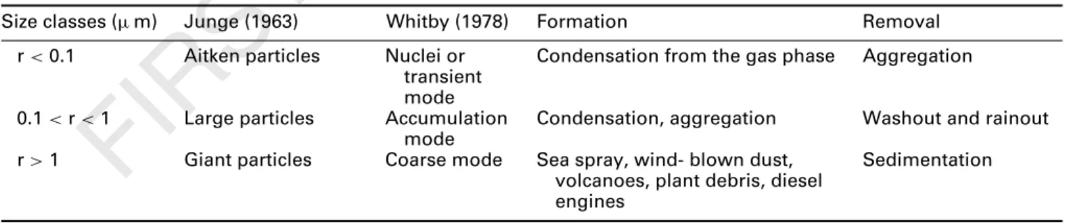
It has been proposed to distinguish three different size ranges for the particles corresponding to different formation and destruction mechanisms:
Table 1 points out that Aitken and large aerosol particles are formed by condensation processes from the gas phase and aggregation. The gases can be of natural or anthro-pogenic origin. However, giant aerosol particles have a mechanical origin, which is mostly natural.
Depending on their size, chemical composition and the ambient relative humidity aerosol particles take up a certain amount of water (K¨ohler curve, see Pruppacher and Klett, 1997). So even in the absence of a cloud, the atmosphere is full of tiny droplets representing swollen aerosol particles, which can become visible, for example, in an atmospheric haze.
At a given size, particles carrying more hygroscopic material can take up more water before achieving a critical size at a critical relative humidity (supersaturation below 5%). When a given aerosol particle has passed its critical size, we call it activated. It serves as a cloud condensation nucleus (CCN). Then, it does not require a further increase in relative humidity to make it grow and it is considered a cloud droplet as long as supersaturation prevails. At a given
ambient supersaturation, all aerosol particles whose critical supersaturation is below the ambient one will be activated and transformed into drops.
Condensation and Evaporation
Once moist aerosol particles have been activated to form drops, they grow according to the droplet growth equation
dmcon/eva dt = ! svw− 2Mwσs,a RT ρwr − υφsεvMwρsrN3 Msρw(r3− rN3) " fv ρwRT esat,wDv′Mw + lvwρw K′T ! lvwMw RT − 1 " (1)
Equation (1) describes the change of the drop mass m (radius r) as a function of the supersaturation svw=
ea/esat,w (ratio of the vapor pressure and the saturation
vapor pressure). Herein, T : temperature, lvw: latent heat
of evaporation, D′
v: modified diffusion coefficient, K′:
modified thermal conductivity, σs,a: surface tension of
the solution droplet, ρw, ρs: density of water and salt
respectively, Mw, Ms molecular weight of water and salt,
ν: number of ions, φs: osmotic coefficient, R: universal
gas constant, εv: mass fraction of soluble material, rN:
radius of the insoluble aerosol nucleus, fv: is the ventilation
coefficient which is due to the falling motion of drops in the atmosphere (for more information see Pruppacher and Klett, 1997).
The growth rates given by this formula are rapid for small droplets.•However, they decrease with an increasing Q3
radius and reduce considerably for drops larger than 10 µm radius (see Pruppacher and Klett, 1997). Consequently, the larger the drop, the longer it will take for it to grow further, leading to a halt in growth by condensation at around 30 µm in radius. Consequently, in order to form precipitation-sized drops other growth mechanisms interfere as detailed below.
Fall Speed of Drops
The terminal velocity of a drop is determined by a balance between buoyancy-corrected gravitation and the drag force
Table 1 Classification of aerosols after Junge and Whitby and the different formation and removal processes most
important for the various size classes of aerosol particles
Size classes (µ m) Junge (1963) Whitby (1978) Formation Removal
r < 0.1 Aitken particles Nuclei or transient mode
Condensation from the gas phase Aggregation 0.1 < r < 1 Large particles Accumulation
mode Condensation, aggregation Washout and rainout r > 1 Giant particles Coarse mode Sea spray, wind- blown dust,
volcanoes, plant debris, diesel engines
FIRST PAGE PROOFS
Table 2 Approximate fall velocities of water drops for the conditions at the surface (1013 hPa, 20◦C)
Radius (r) in µm 50 100 200 500 1000 2000
Terminal velocity (V∞) in ms−1 ∼0.25 ∼0.8 ∼1.5 ∼4 6.5 8.5
acting on the drop. In Table 2, some values for the terminal velocity as a function of drop radius are given.
These values pertain to normal surface conditions. At higher altitudes the fall speed increases as a result of a decrease in air density. These fall speeds are determined in wind tunnel measurements because an analytical calculation using the balance between the acting forces is not possible. This is due to the fact that large drops are no longer spherical. They get deformed by the airstream and develop an indentation on the upwind side. Furthermore, they start to oscillate because of internal and external vortices that develop and because of electrical charges in the atmosphere and the drop. These features do not allow a correct analytical formulation of the drag.
Collision and Coalescence of Drops
Because of the difference in their size, drops have different terminal velocities. Thus, they can overtake each other while falling and collide to form a larger drop with the sum of the original masses. The probability for a small drop r2 that is located inside the geometrical sweep-out volume
of the larger drop r1 to collide with this drop is given
by the collision efficiency Ecoll (Figure 1). This collision
efficiency is strongly dependent on the size of the two drops. If the large drop is smaller than 20 µm, a collision is essentially impossible, as the terminal velocity is too small and the small drop is just carried around the large drop by the airstream. In a wide-size range, the collision efficiency takes values of unity. When the two drops are roughly of equal size, Ecollcan even exceed unity because of the wake
capture of the trailing drop (see Pruppacher and Klett, 1997, for details). Ecoll= πy 2 c π(r1+ r2)2 (2) yc r1 + r2 r1 r2 p(r1 + r2)2 pyc2 Ecoll = (2)
Figure 1 Schematical display of the collision efficiency
The process of collision is not always accompanied by coalescence, a fact that is described by the coalescence efficiency. Colliding drops may bounce apart, coalesce, coalesce temporarily, and then separate again later, or coalesce temporarily and then shatter.
The collection efficiency of the process of drop–drop collision can be written as the product of the collision and the coalescence efficiency:
E(m1, m2)= EcollEcoal (3)
and this efficiency will determine the rate of precipitation formation in clouds that do not develop an ice phase.
It is important to note that collection is enhanced by a broad droplet size spectrum that depends essentially on the dynamics of the clouds but also on the nature and sizes of the aerosol particles, as well as turbulence in clouds, and even radiative cooling effects. The broadness of the distribution is influenced not only by the number of CCN but also by the presence of giant or ultragiant particles, which can serve as coalescence embryos.
Breakup of Drops
Drops in the atmosphere do not grow indefinitely. The upper size limit is around 6 mm in diameter. Drops arriving at this size range develop a tendency to break up. We can distinguish two main mechanisms:
– Spontaneous breakup:the deformation of large drops and the induced oscillation becomes so important that the drop becomes hydrodynamically unstable and breaks up – Collisional break up: during the process of colli-sion/coalescence, the newly formed drop is too unstable and breaks up forming two large drops, slightly smaller than the original drops, and a number of small satellite droplets (see discussion on coalescence above)
Nucleation of Ice Particles
In the atmosphere, liquid drops can exist even at tempera-tures well below 0◦C, that is, in a supercooled state. In fact,
significant numbers of ice particles start to form only below −5◦C coexisting mostly still with liquid drops.
Homo-geneous freezing of liquid droplets depends on the size; large droplets can freeze homogeneously at temperatures of around −33◦C, whereas by −40◦C even the smallest
droplets freeze homogeneously. Thus, at −40◦C the last
FIRST PAGE PROOFS
−5 and −40◦C, the presence of ice-forming nuclei is
nec-essary to initiate the formation of an ice crystal. These ice nuclei (IN) are aerosol particles that can act in four main ways:
– Deposition mode: water is adsorbed directly from the vapor phase onto the surface of an IN where it is transformed into ice
– Condensation–freezing mode: this is a hybrid process that requires supersaturation with respect to water. Here, the CCN that has formed the drop acts now as an IN. This process seems far more effective than the deposition mode.
– Freezing mode: the IN, scavenged by the drop, initiates the ice phase from within a supercooled water droplet – Contact mode: the IN initiates the ice phase at the
moment of contact with the supercooled drop
The number of IN depends on the chemical properties of the aerosol particles. It has been found that there exists a dependency on supersaturation (Meyers et al., 1992) and also on temperature (Fletcher, 1962).•In contrast to CCN,
Q4
a good IN should be insoluble and dispose already of a crystalline-type structure to facilitate the formation of the ice lattice (e.g. silicate). Some bacteria have also been identified as excellent IN. For a comprehensive review of the biogenic versus anthropogenic sources of IN, see Szyrmer and Zawadzki (1997).
Deposition and Sublimation
Water droplets in the atmosphere have a spherical appear-ance facilitating their analytical treatment. Ice crystals present more problems since they appear in a number of different shapes depending on temperature and the grade of water supply. Here we find densely packed structures like needles, columns, and plates, as well as light dendritic struc-tures (for details see e.g. Pruppacher and Klett, 1997). The actual growth rate of these crystals by water vapor depo-sition depends on the crystal form as well as temperature and humidity.
This deposition growth can take place at the same time as the condensation growth of droplets, if the ambient relative humidity is high enough to maintain supersaturation over liquid-water and over ice.•However, the equilibrium curves
Q5
of H2O allow also the case that the air is supersaturated with
respect to ice and subsaturated with respect to liquid water. Then, the drops evaporate and the vapor condenses onto the ice crystals (Bergeron–Findeisen effect; Pruppacher and Klett, 1997).
Fall Speed of Ice Particles
Ice particles like droplets have a terminal velocity that depends heavily on the size of the particle. Additionally,
they depend on the shape of the particle and its density, which can take values between 0.98 g cm−3and 0.2 g cm−3.
A light dendritic structured ice particle will, thus, have a lower terminal velocity than a dense plate-like crystal even if both have the same diameter. For aggregated and rimed structures, the same applies.
Aggregation and Riming
For droplets we noted that condensation alone cannot develop precipitation, and we need the process of colli-sion/coalescence.•The same applies for ice crystals. Their Q6
growth by deposition of water vapor alone is also limited. Thus, a process of collision is necessary to produce larger aggregates. Two different mechanisms are possible: – The collision of ice crystals among themselves: this
process is called aggregation. It is responsible for the formation of snow crystals. This process is efficient in two different temperature regimes, around −10 to −15◦C and around 0◦C. Around −10 to −15◦C, the
crystals develop a dendritic structure and, thus, upon the collision of two crystals they easily succeed in interlinking with their branches. Around 0◦C, the crystals
develop a “pseudo liquid layer” (a micro layer of melting ice) at their surface which enables them to create a link with the other crystal via freezing. Outside these specific temperature regions, the collision of two ice crystals is rarely successful, thus, not resulting in a snow flake. – The collision of ice crystals with liquid drops:this process
is called riming. Here, the drop is frozen upon collision with the crystal and several of these collisions transform the ice crystal into a graupel and then into a hail particle. This is a very efficient way of precipitation production. Sometimes the latent heat involved in this riming process is so important that not all the total captured liquid can be frozen. Normally, the remaining liquid will be incorporated into the solid structure forming a “spongy” ice. In a current meso-scale model(MSL), this is not treated. Thus, the excess liquid is shed and reattributed to the liquid water, a process called wet growth.
Secondary Ice Particle Formation
During the above-discussed processes of aggregation and riming, an ice multiplication mechanism can occur. If the crystals involved in the collision have a dendritic structure, parts can easily break off and form new ice crystals. Hallett and Mossop (1974) also proposed a process leading to secondary ice formation during the process of riming. If the drop involved freezes from the outside-in, then first a solid shell will form with a liquid core. When the liquid core starts to freeze, the volume inside the ice shell is too small to receive the forming ice. This fact will explode the shell and eject liquid material in the air, which will
FIRST PAGE PROOFS
immediately freeze and form new ice crystals. This process is called splintering.
Melting
Even though a precipitating particle might have formed through riming of ice crystals, it can arrive at the ground as a liquid raindrop. This depends on the altitude of the 0◦C
level in the atmosphere. Below this level, ice aggregates will start to melt and, depending on the fall distance, will arrive at the ground as partly or completely melted hydrometeors. A 3-mm ice particle can fall at a distance between 1 and 3 km before complete melting, depending on its initial density and its warm environment (see Pruppacher and Klett, 1997, for details).
THE SCALE PROBLEM
Models are an assembly of equations that describe the phenomenon to be studied. For a cloud model, this includes equations describing the change in time of temperature, humidity, pressure, density, and three-dimensional (3-D) wind field, and some variables that represent the cloud, such as drop or crystal numbers or liquid water content. These equations emerge from the concepts of conservation of mass and energy, Newton’s law, and the perfect gas law and can be written in a general form:
∂ρ ∂t + div(ρ ⃗v) = 0 ∂T ∂t + div(ρ ⃗vT ) = 1 cp div ⃗FT + 1 ρcp dp dt + L cpCcon +Lsub cp Csub+ Lmelt cp Cmelt ∂
∂tρ⃗v + div(ρ ⃗v⃗v) = gr ⃗ad p − ρ ⃗g + divτ ∂
∂tρqv+ div(ρ ⃗vqv)= div ⃗Fv− Ccon− Csub− Cmelt ∂Ndrop
∂t + div(⃗vNdrop)+ ∂
∂z(V∞,dropNdrop) = div ⃗Fdrop+ Sdrop
∂Ncrystal
∂t + div(⃗vNcrystal)+ ∂
∂z(V∞,crystalNcrystal) = div ⃗Fcrystal+ Scrystal
p/ρ = nRT (4)
with ρ: density of air, ⃗v: 3-D wind field, T : temperature, qv: water vapor mixing ratio, cp: specific heat at constant
pressure, ⃗FT: sensible heat-flux, p: pressure, L, Lsub,
Lmelt: latent heat of condensation, sublimation, and melting,
Ccon, Csub, Cmelt: rate of phase change of condensation,
sublimation, and melting, ⃗g: acceleration of gravity, τ: friction tensor, Ndrop, Ncrystal: number of drops and crystals
of a given size per unit volume, ⃗Fdrop, ⃗Fcrystal: diffusion
fluxes of drops and crystals, Sdrop, Scrystal: source, sinks, and
transfer terms of drops and crystals, n: number of moles, R: universal gas constant. (Instead of temperature, models often calculate potential temperature θ = T (p0/p)(R/cp).)
These equations are, then, solved numerically at a number of points in space and time, while the points represent a certain interval in time or space. As the equations result from continuity principles, these intervals should be infinitely small. In practice, the grid boxes have a finite size. Thus, to be correct, we need to average the equations over finite increments in space and time:
ψ= 1 ,t,x,y,z # t+,t t # x+,x x # y+,y y # z+,z z ψdz dy dx dt ψ = ψ + ψ′ (5)
This modifies the equations in such a way that we now calculate average values over a grid box that modifies the equations so that a new term appears in every prognostic equation taking into account the subgrid changes of space and time inside the box:
∂ρ ∂t + div(ρ ⃗v) = 0 ∂T ∂t + div(ρ ⃗vT ) − div ⃗F turb T = 1 cpdiv ⃗FT + 1 ρcp dp dt + L cpCcon+ Lsub cp Csub+ Lmelt cp Cmelt ∂ ∂tρ⃗v + div(ρ ⃗v⃗v) − divτ
turb = gradp − ρ ⃗g + divτ
∂
∂tρqv+ div(ρ ⃗vqv)− div ⃗F
turb
v = div ⃗Fv
− Ccon− Csub− Cmelt
∂Ndrop
∂t + div(⃗v Ndrop)+ ∂
∂z(V∞,dropNdrop) − div ⃗FN dturb= div ⃗Fdrop+ Sdrop
∂Ncrystal
∂t + div(⃗v Ncrystal)+ ∂
∂z(V∞,crystalNcrystal) − div ⃗FN cturb= div ⃗Fcrystal+ Scrystal
p/ρ = nRT (6)
The new terms have the form: ⃗
FIRST PAGE PROOFS
and depend on the subgrid fluctuations ψ′ in space and
time of the considered variables. These terms need to be parameterized as a function of the variables ψ of the resolved scale. This approach is known under the term
closure, whereby different theories of closure (first, second order, etc.) can be found in the literature Stull (1991). In the following, for simplicity of writing, the overbar will be dropped; however, all equations are averaged equations.
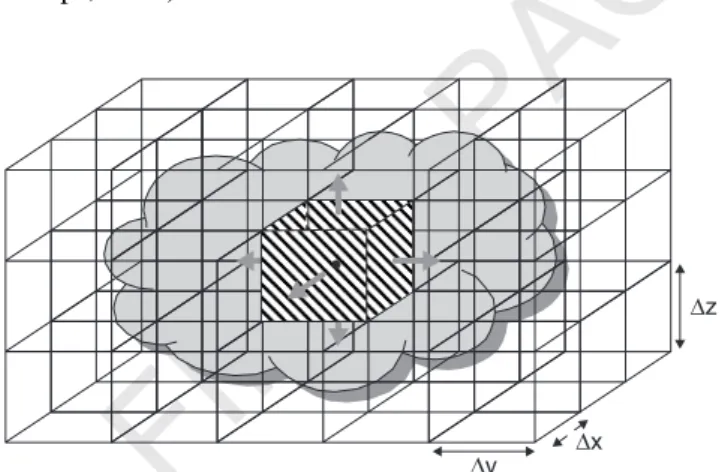
Considering, that an appropriate closure approach has been selected, the foregoing equations can be solved numer-ically in a type of grid such as that displayed in Figure 2, covering the entire cloud area and the affected environ-ment. The averaging done in equations (6) and (7) now allows finite grid increments. However, the microphysical processes discussed above make it evident that essential processes in clouds operate at the scale of micrometers, requiring very small intervals in space. But, on the other hand, clouds sometimes form systems of several thousand kilometers, requiring a large spatial domain to be cov-ered. One is, thus, confronted with the problem that actual computer power does not allow us to cover domains of 1000 km2 with grid increments of 1 m2 (this would require
1012 grid boxes).
A similar argumentation applies to the time incre-ment. Time and space increments are linked in an explicit numerical treatment of the system of equations by the Courant–Friedrich–-Levy (CFL) criterium (Jacobson,
1999): !
,t ,x
"
U ≤ 1 (8)
with U being the maximum transport velocity considered. This criterium insures that the fasted signal does not jump a grid box in one time step. The fasted transport velocities in the atmosphere are those of the sound. They are not physically relevant in cloud models and are, thus, filtered by suppressing local density fluctuations in the equations (an elastic or soundproof assumption) (Ogura and Phillips, 1962).
∆x ∆y
∆z
Figure 2 Scheme of grid boxes that resolve a cloud
However, the numerical effort for a high resolution of the processes stays considerable. Consequently, strategies to reduce the simulation time need to be developed. These consist in compromises concerning the dynamics, the microphysics, and the resolution.
SIMPLIFICATION IN THE DYNAMICS
3-D Models
The appropriate way to simulate the dynamics of the atmosphere is a 3-D representation of space. Here, a classical coordinate system would be a Cartesian one with x, y, and z in the directions of space (see Figure 2). In order to take into account the topography, often the vertical coordinate z is replaced by one that follows the terrain. Phillips (1957) designed such a terrain-following coordinate system for use in hydrostatic, numerical prediction models by defining:
σ = p
ps (9)
where ps represents surface pressure and σ varies from
a value σ = 1 at the ground to σ = 0 at the top of the atmosphere. Nowadays, however, most of the 3-D models (Clark, 1977; Dudhia, 1993; Pielke et al., 1992) devoted to cloud simulations use the vertical coordinate:
z∗= H z− zs H− zs
(10) The surface height above some reference level is given by zs (e.g. sea level) and the height of the model top is
given by H .
Three-dimensional models that cover an entire continent equally need to take into account in the horizontal grid the deformation of the coordinate system by the curvature of Earth and the large-scale Coriolis force. These models use stereographic coordinate systems. Some of the most widely used 3-D models are currently RAMS (Pielke et al., 1992; Cotton et al., 2003), MM5 (Dudhia, 1993), and Clark (1977), among others.
2-D Models
For special case studies concerning phenomena that are mainly two-dimensional (2-D; flow over a mountain range, e.g.) or in order to reduce computer calculation times, 3-D dynamics can be reduced to two dimensions. This eliminates one coordinate (e.g. y in a Cartesian coordi-nate system) (e.g. Orville and Kopp, 1977; Soong and Ogura, 1980)
Another configuration, especially adapted in simulating isolated cumulus clouds consists of a cylindrical model with a symmetry with respect to the angular coordinate. Such
FIRST PAGE PROOFS
a model configuration has been used, for example in the models of Shiino (1983), Murray and Koenig (1975), and Reisin et al. (1996).
1-D and 0-D Models
The cylindrical model philosophy has also been applied in the 1.5-D model of Asai and Kasahara (1967) where in fact two one-dimensional models are connected to represent the updraft and the downdraft region of a convective cloud.
Nowadays, one-dimensional models are mainly used to test microphysical schemes. In this case, there exists just a vertical axis z, subdivided into several layers, representing the updraft region of the cloud.
Finally, the least sophisticated dynamics is that of an air parcel. In this concept, we consider a volume of air separated from the environment by an immaterial surface. For the entraining air parcels, they exchange mass and heat with the environment; otherwise, they are considered as adiabatic. Air parcels can represent an interesting concept if they are driven by a 3-D flow field, because they permit highly resolved microphysics to be followed in a larger-scale dynamics that does not consider microphysics (Feingold et al., 1998a). Here, care needs to be taken to ensure that the parcel bulk properties are adequately constrained to those from the driving 3-D model.
MODELS OF CLOUD MICROPHYSICS
Drops and ice crystals exist in a cloud in varying number concentrations and with different sizes. We distinguish cloud drops of radii between 1 µm and 30 µm, drizzle drops of up to 200 µm, and rain drops up to 6 mm. Ice crystals have diameters of up to 100 µm, snow flakes, graupel, and hail particles have no clear upper size but can become larger than raindrops. The number of hydrometeors per unit volume of a given size is fundamental for the evolution of the cloud and, thus, should be considered in a cloud model.
Explicit or Bin-resolving Cloud Models
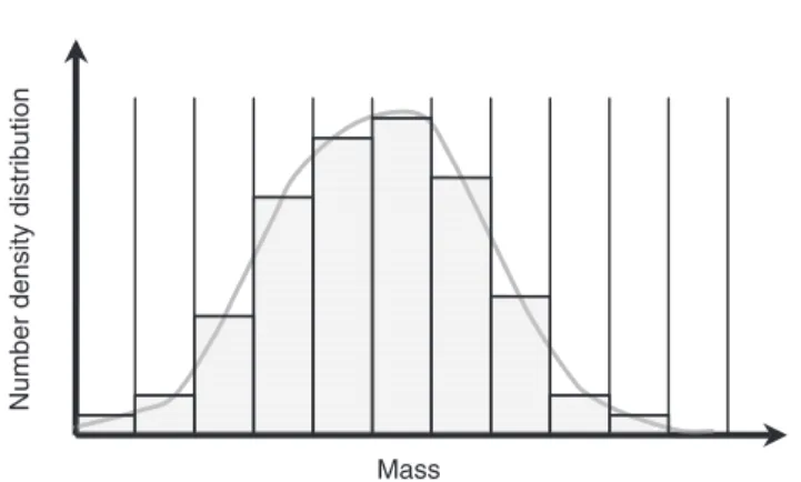
The most logical approach is to introduce an explicit number density distribution function f (m) dm, which follows the number per unit volume of a given type of hydrometeors in a given mass class between m and m+ dm (see Figure 3). Inside a bin, class most models assume a uniform value. There exist, however, also models that assume inside a drop bin class a distribution of aerosol particles or chemical compounds (e.g. Wobrock
et al., 2002). Warm Clouds
Most ground fogs or low-level clouds contain only liquid drops, and no ice crystals. If they develop precipitation, this
Number density distribution
Mass
Figure 3 Number density distribution function f (m) dm which follows the number per unit volume of air of a given type of hydrometers in a given mass class betweenm and m + dm
will take place by the collision and coalescence of liquid drops. These clouds are called warm clouds. In order to model the size distribution of droplets in warm clouds, a drop number density distribution function fd(m)is defined.
It allows the continuous distribution of drops over the entire spectrum to be captured in a discrete function.
Since the liquid hydrometeors need to cover a range from 1 µm drops up to 6 mm raindrops, which covers at least three orders of magnitude, an equidistant grid in size or mass is not appropriate. Consequently, Berry and Reinhardt (1974a–c) have introduced a logarithmic size grid which allows a doubling of mass every JRS category:
r(j )= r(1)2(J−1)/3J RS (11) r(1) gives the minimum radius (e.g. 1 µm) and JRS can be 1, 2, 3, or more. In most models J RS= 2 is chosen, as a compromise between the necessary resolution of drop spectrum (Silverman and Glass, 1973) and the computer times of the simulation. For each of the resulting drop-size classes (on the order to 70), the following prognostic equation has to be solved:
∂fd(m,⃗r, t) ∂t = −div(⃗vfd(m,⃗r, t)) + ∂ ∂z(V∞fd(m,⃗r, t)) + div( ⃗F turb f d ) + $ ∂ ∂tfd(m,⃗r, t) % nuc+ $ ∂ ∂tfd(m,⃗r, t) % con/eva + $ ∂ ∂tfd(m,⃗r, t) % coll+ $ ∂ ∂tfd(m,⃗r, t) % breakup (12) The term on the left-hand side calculates the change of the number of drops at a certain location⃗r per unit volume between a mass m and m+ dm per time interval dt because
FIRST PAGE PROOFS
of the physical effects represented by the terms on the right-hand side which are: transport with the scale velocity ⃗v, the sedimentation with the terminal velocity V∞, transport through turbulence, the change in number concentration due to nucleation of drops, due to condensation or evaporation, due to collision and coalescence among the drops, and due to breakup of drops. The mathematical expressions for these terms follow the physics detailed above.
A simple way to calculate the nucleation of drops is to prescribe the number of cloud condensation nuclei as a function of supersaturation:
NCCN= csvwk (13)
with c, k constants which are adapted to the air mass considered, as, for example, in Twomey (1959). In addition, an assumption is necessary on the size of the freshly nucleated drops. More sophisticated models (Flossmann
et al., 1985) follow the number of aerosol particles and their chemical composition in order to calculate as a function of supersaturation (K¨ohler equation, Pruppacher and Klett, 1997) the number and the size of activated aerosol particles. Once formed, the drops grow or shrink by condensation or evaporation respectively: $ ∂ ∂tfd(m) % con/eva= − ∂ ∂m ! dmcon/eva dt fd(m) " (14) where the individual droplet growth rate is given from equation (1). The process of collision and coalescence of drops is calculated following Berry and Reinhardt (1974a–c): $ ∂ ∂tfd(m) % coll= # m/2 0 fd(m− m ′)f d(m′)K(m− m′, m′)dm′ − # ∞ 0 fd(m)fd(m′)K(m, m′)dm′ (15)
Here, the first term on the right-hand side describes the gain of m-sized drops due to collision between drops of sizes (m− m′)and m′. The second term describes the loss
of m-sized drops due to all types of collision. K represents the coalescence kernels that give the probability of such a collision to happen. E is the collection efficiency.
K(m, m′)= π(r + r′)|V∞,drop(m)
− V∞,drop(m′)| E(m, m′) (16)
The breakup term can be parameterized either as a spontaneous breakup (see e.g. Hall, 1980; Srivastava, 1971) or as a collisional breakup (Low and List, 1982a,b).
In solving these equations coupled with the 1, 2, or 3–D dynamics as detailed above, the calculation of the
evolution of the drop-size distribution as a function of time and space inside and below the cloud, as well as on the ground is allowed.
However, because of the large number of variables to be updated at every time step, only a few models available can calculate explicit cloud microphysics in a 3-D framework (e.g. Feingold et al., 1994 Kogan, 1991 Khvorostyanov, 1995). Most models are restricted to two dimensions (Hall, 1980) or – one dimension (Ogura and Takahashi, 1973). The parcel model discussed above is an exception, since it does not allow precipitation to be calculated. It can, thus, only be used to simulate the evolution of a nonprecipitating cloud •(Feingold et al., 1998), or at the most estimate the Q7
amount of precipitable water. Cold Clouds
Most clouds in midlatitudes form ice particles and the formation of precipitation involves the ice phase. The ice phase can also be modeled by a bin approach if a certain number of additional size distributions are considered – one distribution function to follow the pristine (non or little rimed) crystals: fi, one distribution function for the
heavily rimed particles like graupel or hail fh, and one
distribution function for snow flakes, that is, aggregates of crystals fs. As ice particles generally can become
larger than liquid drops, more categories need to be considered. Also, because of the different possible forms of ice crystals (columns, needles, plates, etc.) additional distribution functions can be added. However, most models follow just one species of crystal shape (plate-like; e.g. Alheit et al., 1990). Only a few models calculate the explicit cold microphysics in three-dimensions (Ovtchinnikov and Kogan, 2000). Most models use reduced dynamics, for example, 2-D (Respondek et al., 1995), 1 – D, or parcel models (Alheit et al., 1990). Takahashi had the first paper on bin-resolved microphysics of mixed-phase clouds in the 1970s. Reisin et al. (1996) is another review on mixed-phase bin models of considerable sophistication. It has been used in 2-D models of cumuli and also Arctic stratus clouds (Harrington et al., 2000).
Bulk Parameterizations
Between 1965 and 1975, when cloud modeling started, due to the limitations of early computers, bin modeling in a reasonable dynamic framework was completely out of reach.
Warm Clouds
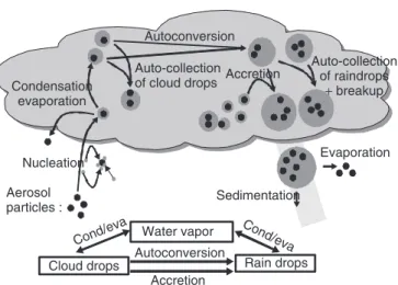
Consequently, Kessler (1969) proposed a simple parame-terization of the microphysics of a warm cloud (Figure 4).
FIRST PAGE PROOFS
Nucleation
Autoconversion Auto-collection
of cloud drops Accretion
Auto-collection of raindrops + breakup Aerosol particles : Condensation evaporation Evaporation Water vapor
Cloud drops Autoconversion Rain drops Accretion
Cond/eva
Cond/eva
Sedimentation
Figure 4 Schematic display of warm cloud processes and
the simplification of the Kessler parameterization
It aimed to simulate a convective cloud and just calculated the amount of liquid water attached to the small, nonprecip-itating drops (r smaller than 50 µm) and the amount of liquid water attached to precipitation-sized drops (r larger than 50 µm). However, due to its simplicity this scheme was quickly adapted to all types of clouds, and still has its place in many weather prediction models.
The basic equations of this model allow calculation of the evolution with time of the water vapor mixing ratio qv,
the cloud water mixing ratio qc, and the rain water mixing
ratio qR. ∂ρqv ∂t = −div(⃗vρqv)+ div( ⃗F turb v ) − Ccon,c+ Ceva,R ∂ρqc ∂t = −div(⃗vρqc)+ div( ⃗F turb c )
− Pauto− Pacc+ Ccon,c
∂ρqR
∂t = −div(⃗vρqR)+ ∂ ∂zVRρqR
+ div( ⃗FRturb)+ Pauto+ Pacc− Ceva,R (17)
Here, Kessler (1969) proposes for the condensation rate of cloud drops Ccon,c a saturation adjustment. This
means that all dynamically generated supersaturation is immediately converted to cloud water. And in cases of subsaturation, an amount of cloud water is evaporated that restores saturation, if possible. Obviously, this is a rather crude treatment that does not consider the role of the CCN population and the supersaturation.
Pauto is the autoconversion rate, that is, the collision
of cloud water that forms rain water. It is assumed to be a linear function of the cloud water content, only influenced by threshold values qcrit determining the onset
of the autoconversion process. In the literature, numerous different values for qcrit have been proposed.
Pauto= k(ρqcrit− ρqc) k= 10−3s−1if ρqc> ρqcrit,
otherwise k= 0 (18)
The accretion rate Pacc details the amount of rainwater
created by further collision with cloud water. Kessler (1969) calculates the accretion rate by:
Pacc =
# ∞ 0
dmacc
dt NR(r)dr (19) by calculating the increase of mass of one raindrop macc of
radius r due to the collision with a cloud water population Water vapor qV Suspended drops qC Suspended cloud ice qCI Raindrops qR Hail Ni = 1..21 Autoconversion Accretion Cond/eva Evaporation Hom. or het. nucleation Melting Riming « Bigg » freezing Autoconversion Diffusion growth Riming Wet growth Diffusion Melting Sublimation
Figure 5 •Scheme of the interaction taken into account in a hybrid scheme combining a bulk approach for cloud water,
Q2
FIRST PAGE PROOFS
presumed monodisperse represented by qc with a collision
efficiency of E. dmacc
dt = πr
2
EVR(r)ρqc (20)
In assuming that the raindrops obey a Marshall–Palmer distribution, (Marshall and Palmer, 1948):
NR(r)= NR,0e−2λr (21)
where λ: shape parameter, and assuming a simple analytical function for the drop terminal velocity:
VR(r)= 130 √ 2r (22) yielding VR= # ∞ 0 VR(r)NR(r)dr # ∞ 0 NR(r)dr (23) in m s−1.
Autocollection of cloud or raindrops are not considered in this approach. The evaporation rate of raindrops below cloud base can be calculated by
Ceva,R= −# dmcon/evadt NR(r)dr (24)
Numerous authors have since modified the terms for the parameterizations of the different processes, keeping, however, the basic concept (Berry,1965; Orville and Kopp, 1977, among others).
Cold Clouds
The basic concept of the warm cloud bulk parameterization was soon extended to cold clouds, distinguishing two or three categories of ice. One, corresponding to nonprecipi-tating cloud drops is called cloud ice. For the precipinonprecipi-tating cloud ice, one can, for example, distinguish graupel from
snow.
An example for cloud ice and graupel can be found in Orville and Kopp (1977), an example for cloud ice, graupel, and snow can be found in Lin et al. (1983), and an example using pristine, such as non- or little-rimed crystals (ice A) and rimed crystals (ice B) can be found in Koenig and Murray (1976). A new approach to couple bulk and explicit microphysics can be found in Farley and Orville (1986), which was recently applied to a 3-D model (Wobrock et al., 2003). It should be mentioned that the approach of Farley and Orville is a hybrid approach in which hail is simulated in bins, although continuous accretion approximations are used.
Examples for pure bulk ice physics in a 3-D model can be found in Reisner et al. (1998)and for a 2-D model in Grabowski et al. (1996).
The Semispectral Microphysics Parameterizations
As a compromise between the bin schemes that follow the spectra of hydrometeors in discrete size classes or bins and the bulk parameterizations that follow just the water mass associated to 5 or 6 classes of hydrometeors, recently, semi-spectral parameterizations have been developed.
These parameterizations, similar to the bulk ones, fol-low a limited number of categories. Within one category, however, they assume a size distribution of a log-normal or gamma type, and then calculate the time evolution of the first (total number) and third (mass) moment of these distribution functions. Example of these approaches can be found in Ferrier (1994), Meyers et al. (1997), Cohard and Pinty (2000), Seifert and Beheng (2003), and Caro et al. (2003). Actually, Meyers et al. was already extended to the ice phase. Moreover, their approach used approximate solu-tions or look-up table solusolu-tions to the stochastic collection equations as opposed to the continuous accretion approxi-mations to collection. Subsequently, Feingold et al. (1998b) extended the emulation of a bin model in a bulk scheme to autoconversion and sedimentation.
More recently Saleeby and Cotton (2004) added a sec-ond mode to the cloud droplet spectrum which permitted a more accurate representation of collection (autoconversion) and sedimentation, and permitted the explicit activation of CCN (including a concept for giant CCN) and IN. Others such as Milbrandt and Yau (2004) extended this approach to a three-moment scheme in which all degrees of free-dom in the specified basis functions are predicted. This approach offers an interesting compromise between the detailed bin approach and bulk schemes. The reduction in computational effort will probably mean that even opera-tional forecast models will move towards these schemes in the future.
CUMULUS PARAMETERIZATIONS
If the size of the grid increments becomes larger than 10 km, it is no longer possible to resolve the convective clouds explicitly (stratiform clouds with large horizontal extension can still be resolved). But since the energetic processes associated with convective clouds are important, their net impact on the scale values needs to be parameterized, in addition to the turbulence parameterization already dis-cussed. This gives rise to cumulus parameterizations which can be traced back to the development of numerical predic-tion models. Smagorinsky (1956) was the first to introduce a cumulus parameterization when he adjusted the vertical derivative of an “effective static stability” which included
FIRST PAGE PROOFS
the heat released during condensation. This gave rise to the first approaches of cumulus parameterizations called
con-vective adjustment (e.g. Krishnamurti and Moxim, 1971; Manabe et al., 1965; Kurihara, 1973). As these approaches turned out too crude, a second generation of schemes attempted to link the convection to the large-scale mass, moisture, or energy convergence, while using some form of “cloud model” (mostly rising plumes and compensat-ing downdrafts) to vertically distribute mass, moisture, and energy by a flux scheme (e.g. Kuo, 1965, 1974; Anthes, 1977, Fritsch and Chappel, 1980; Tiedke, 1989). Another large-scale control was introduced by Arakawa and Schu-bert (1974). They assumed that the rate of stabilization by an ensemble of cumulus clouds balances the rate at which the large scale makes buoyant energy available for convec-tion. For a complete review of the approaches, see Emanuel and Raymond (1993).
All cumulus parameterization schemes depend severely on the size of the grid box, which they need to stabilize completely or only partially. Consequently, they will only apply to the case for which they were developed and cannot easily be generalized for other grid sizes.
A recent approach, for example, Grabowski et al. (2001) and Khairoutdinov and Randall (2001) concerns the devel-opment of so-called “super-parameterizations” that have now been implemented in several global circulation mod-els. This approach consists basically in running a 2-D cloud-resolving model at each grid point and average the cloud-resolving model data to determine heating, moisten-ing, and precipitation rates.
NUMERICS
The forgoing physical treatments of the different processes involved in clouds enter the balance equations. These equa-tions, then, need to be solved numerically on a computer. However, before coding, the differential expressions in the terms need to be discretized in order to be linked to the scale variables. The real art of cloud models these days lies here. Numerous studies have been performed on the best numerical scheme to solve the transport equation (positive-definite schemes; e.g. Smolarkiewicz, 1984; Bott, 1989) and the integrals in the drop–drop collision/coalescence process (e.g. Berry and Reinhardt, 1974a-c; Bott, 2000), and it is the best way to distribute the calculated val-ues in a grid, among others. Another serious numerical problem lies in the calculation of the supersaturation due to dynamical and microphysical tendencies. These ten-dencies should be solved at the same time and not one after the other as in the models. As these tendencies are very sensible, they require extremely small time steps, which in connection with the timescales of the other pro-cesses introduce a numerical stiffness problem. Numerous approaches concerning this problem have been proposed
in the literature. Next to the explicit method, implicit methods were also developed. Equally, the state-of-the-art cloud models now dispose of an interactive two-way grid nesting. This allows zooming with finer resolution into a domain of special interest and transferring this information to the larger grid outside afterwards. These techniques create a new way to address the scale prob-lem, in following the large-scale dynamics in a coarse grid and then, to zoom with a finer grid into the cloud region. Another technique that advances cloud model-ing is the assimilation of remote sensmodel-ing data (e.g. from satellite) into a model in order to improve model ini-tialization. Furthermore, the calculated evolution can be constrained by observation or outputs of other models. For a summary of current modeling techniques, see Jacob-son (1999).
CONCLUSION
This article attempts to provide an introduction to the complex subject of modeling clouds, the production of precipitation, and the development of cloud and storm systems. The elements intervening in cloud modeling have been exposed, starting from a description of the physical phenomena. On the basis of the occurring scale problem, a number of approaches for simplification were presented. These parameterizations are generic and can be combined as a function of the addressed problem. In addition, other modules that have not been discussed in the article need to be added, such as a radiation model, a surface model, a chemistry model, and so on. The main problem is achieving a balance between the degree of parameterization, the number of physical and chemical processes relevant to a particular problem, and the available computing resources. Owing to the increasing capacity of computers, however, less and less parameterizations are necessary and the resulting models are more and more complete. Consequently, the current state-of-the-art MSMs (e.g. RAMS, MM5, Clark, etc.) have large capacities. Essentially the same models can be used to study problems as diverse as rainfall over large areas and over many hours, resulting from frontal cloud systems, the development of local storms with damaging hail and flooding, transport of pollutants by small convective clouds, and photochemical reactions in fog. Next to these models a variety of different models exist which are more or less restricted to a specific question.
FURTHER READING
•Takahashi T. (1976) Hail in an axisymmetric cloud model. Q8 Journal of the Atmospheric Sciences, 33, 1579–1601.
FIRST PAGE PROOFS
REFERENCES
Alheit R.R., Flossmann A.I. and Pruppacher H.R. (1990) A theoretical study of the wet removal of atmospheric pollutants. Part IV: The uptake and redistribution of aerosol particles through nucleation and impaction scavenging by growing cloud drops and ice particles. Journal of the Atmospheric Sciences, 47, 870 – 887.
Anthes R.A. (1977) A cumulus parameterization scheme utilizing a one-dimensional cloud model. Monthly Weather Review, 105, 270 – 286.
Arakawa A. and Schubert W.H. (1974) Interaction of a cumulus cloud ensemble with the large-scale environment. Part I.
Journal of the Atmospheric Sciences, 31, 674–701.
Asai T. and Kasahara A. (1967) A theoretical study of the compensating downward motions associated with cumulus clouds. Journal of the Atmospheric Sciences, 24, 487–496. Berry E.X. (1965) Cloud droplet growth by collection. Journal of
the Atmospheric Sciences, 24, 688–701.
Berry E.X. and Reinhardt R.L. (1974a) An analysis of cloud drop growth by collection. Part I: Double distributions. Journal of
the Atmospheric Sciences, 31, 1814–1824.
Berry E.X. and Reinhardt R.L. (1974b) An analysis of cloud drop growth by collection. Part II: Single initial distributions.
Journal of the Atmospheric Sciences, 31, 1825–1831.
Berry E.X. and Reinhardt R.L. (1974c) An analysis of cloud drop growth by collection: Part III: Accretion and self-collection.
Journal of the Atmospheric Sciences, 31, 2118–2126.
Bott A. (1989) A positive definite advection scheme obtained by nonlinear renormalisation of the advective fluxes. Monthly
Weather Review, 117, 1006–1015.
Bott A. (2000) A flux method for the numerical solution of the stochastic collection equation: extension to two dimensional particle distributions. Journal of the Atmospheric Sciences, 57, 284 – 294.
Caro D., Wobrock W., Flossmann A.I. and Chaumerliac N. (2003) A two-moment parameterization of aerosol nucleation and impaction scavenging for warm cloud microphysics: description and two-dimensional results. Atmospheric Research, 70(3 – 4), 171–208, DOI 10.1016/j.atmosres.2004. 01.002.
Clark T.L. (1977) A small-scale dynamic model using a terrain-following coordinate transformation. Journal of Computational
Physics, 24, 186–215.
Cohard J.-M. and Pinty J.-P. (2000) A comprehensive two-moment warm microphysical bulk scheme. Part I: description and selective tests. Quarterly Journal of the Royal
Meteorological Society, 126, 1815–1842.
Cotton W.R. and Anthes R.A. (1989) Storm and Cloud Dynamics, Academic Press: San Diego, p. 880.
Cotton W.R., Pielke R.A. Sr, Walko R.L., Liston G.E., Trem-back C.J., Jiang H., McAnelly R.L., Harrington J.Y., Nicholls M.E., Carrio G.G., •et al. (2003) RAMS 2001: current status Q9
and future directions. Meteorology and Atmospheric Physics,
82, 5–29.
Dudhia J. (1993) A non-hydrostatic version of the PENN State-NCAR meso-scale model: validation tests and simulation of an Atlantic cyclone and cold fronts. Monthly Weather Review, 121, 1493 – 1413.
Emanuel K.A. and Raymond D.J. (1993) The representation of cumulus convection in numerical models. Meteorological
Monographs, Vol. 24, American Meteorological Society. Farley R.D. and Orville H.D. (1986) Numerical modelling of
hailstorms and hailstone growth. Part I: Preliminary model verification and sensitivity test. Journal of Climate and Applied
Meteorology, 25, 2014 – 2035.
Feingold G., Kreidenweis S.M. and Zhang Y. (1998a) Stratocumulus processing of gases and cloud condensation nuclei 1. Trajectory ensemble model. Journal of Geophysical
Research, 103, 19527–19542.
Feingold G., Stevens B., Cotton W.R. and Walko R.L. (1994) An explicit cloud microphysics/LES model designed to simulate the Twomey effect. Atmospheric Research, 33, 207–234. Feingold G., Walko R.L., Stevens B. and Cotton W.R.
(1998b) Simulations of marine stratocumulus using a new microphysical parameterization scheme. Atmospheric Research,
47–48, 505–528.
Ferrier B. (1994) A double moment multiphase four-class bulk ice scheme. Part I: description. Journal of the Atmospheric
Sciences, 51, 249–280.
Fletcher N.H. (1962) The physics of rainclouds, Cambridge University Press: London.
Flossmann A.I., Hall W.D. and Pruppacher H.R. (1985) A theoretical study of the wet removal of atmospheric pollutants. Part I: the redistribution of aerosol particles captured through nucleation and impaction scavenging by growing cloud drops.
Journal of the Atmospheric Sciences, 44, 2912–2923. Flossmann A.I. and Laj P. (1998) Aerosols, gases and
microphysics of clouds, ERCA, Vol. 3, Boutron C.F. (Ed.) EDP Sciences: pp. 90 – 119.
Fritsch J.M. and Chappel C.F. (1980) Numerical Prediction of Convectively driven mesoscale pressure systems. Part I: convective parameterizations. Journal of the Atmospheric
Sciences, 37, 1722–1762.
Grabowski W.W. (2001) Coupling cloud processes with the large-scale dynamics using the cloud-resolving convection parameterization (CRCP). Journal of the Atmospheric Sciences,
58, 978–997.
Grabowski W., Wu X. and Moncrieff M.W. (1996) Cloud resolving modelling of tropical cloud systems during Phase III of GATE. Part I: two-dimensional experiments. Journal of the
Atmospheric Sciences, 53, 36843709.
Hall W.D. (1980) A detailed microphysical model within a two-dimensional dynamic framework: model description and preliminary results. Journal of the Atmospheric Sciences, 37, 2486 – 2507.
Hallett J. and Mossop S.C. (1974) Production of secondary ice particles during the riming process. Nature, 249, 26–28.
Harrington J.Y., Reisin T., Cotton W.R. and Kreidenweiss• Q10 S.M. (2000) Cloud resolving simulations of arctic stratus Part II: transition-season clouds. Atmospheric Research, 55, 45 – 75.
Houze R.A. (1993) Cloud dynamics, Academic Press: San Diego. Jacobson M.Z. (1999) Fundamentals of Atmospheric Modelling,
Cambridge University Press: p. 656.
Junge C.E. (1963) Air Chemistry and Radioactivity, Academic Press.
FIRST PAGE PROOFS
Kessler E. (1969) On the distribution and continuity of water substance in atmospheric circulations. Meteorological
Monographs, Vol. 32, American Meteorological Society:
Boston.
Khairoutdinov M.F. and Randall D.A. (2001) A cloud resolving model as a cloud parameterization in the NCAR community climate system model: preliminary results. Geophysical
Research Letters, 28, 3617–3620.
Khvorostyanov V.I. (1995) Meso scale processes of cloud formation, cloud-radiation interaction and their modelling with explicit cloud microphysics. Atmospheric Research,
48, 1–67.
Koenig L.R. and Murray F.W. (1976) Ice-bearing cumulus cloud evolution. Numerical simulation and general comparison against observation. Journal of Applied Meteorology, 15, 747 – 762.
Kogan Y.L. (1991) The simulation of a convective cloud in a 3-D model with explicit microphysics. Part I: model description and sensitivity experiments. Journal of the Atmospheric Sciences,
48, 1160–1189.
Krishnamurti T.N. and Moxim W.J. (1971) On parameterization of convective and non convective latent heat release. Journal
of Applied Meteorology, 10, 3–13.
Kuo H.L. (1965) On the formation and intensification of tropical cyclones through latent heat release by cumulus convection.
Journal of the Atmospheric Sciences, 22, 40–63.
Kuo H.L. (1974) Further studies of the parameterization of the influence of cumulus convection on large-scale flow. Journal
of the Atmospheric Sciences, 31, 1232–1240.
Kurihara Y. (1973) A scheme of moist convective adjustment.
Monthly Weather Review, 101, 547–553.
Lin Y.L., Farley R. and Orville H. (1983) Bulk parameterization of the snow filed in a cloud model. Journal of Climate and
Applied Meteorology, 22, 1065–1092.
Low T.B. and List R. (1982a) Collision, coalescence and breakup of raindrops: Part I: experimentally established coalescence efficiencies and fragment size distribution in break up. Journal of the Atmospheric Sciences, 39, 1591 – 1606.
Low T.B. and List R. (1982b) Collision, coalescence and break up of raindrops: Part II: parameterizations of fragment size distributions. Journal of the Atmospheric Sciences, 39, 1607 – 1618.
Manabe S., Smagorinsky J. and Strickler R.R. (1965) Simulated climatology of a general circulation model with a hydrological cycle. Monthly Weather Review, 93, 769 – 798.
Marshall J.S. and Palmer W.M. (1948) The distribution of raindrops with size. Journal of Meteorology, 5, 165 – 166. Meyers M., DeMott P.J. and Cotton W.D. (1992) New primary
ice-nucleation parameterization in an explicit cloud model.
Journal of Applied Meteorology, 31, 708–721.
Meyers M., Walko R., Harrington J. and Cotton W. (1997) New RAMS cloud microphysics parameterization. Part II: the two-moment scheme. Atmospheric Research, 45, 3 – 39.
Milbrandt J. and Yau M.K. (2004) Analysis of the role of the shape parameter in bulk microphysics parameterization and a proposed triple-moment approach. Journal of the Atmospheric
Sciences,•in press. Q11
Murray F.W. and Koenig L.R. (1975) Cumulus cloud energetics as revealed in a numerical model of cloud dynamics: Part I. Theoretical development.•Pageoph., 113, 909–923. Q12 Ogura Y. and Phillips N.A. (1962) Scale analysis of deep
and shallow convection in the atmosphere. Journal of the
Atmospheric Sciences, 19, 173–179.
Ogura Y. and Takahashi T. (1973) The development of warm rain in a cumulus model. Journal of the Atmospheric Sciences, 30, 262 – 277.
Orville H.D. and Kopp F.J. (1977) Numerical simulation of the life history of a hailstorm. Journal of the Atmospheric Sciences,
34, 1596–1618.
Ovtchinnikov M. and Kogan Y.L. (2000) An investigation of ice production mechanisms in small cumuliform clouds using a 3-D model with explicit microphysics. Part I: model description.
Journal of the Atmospheric Sciences, 57, 2989–3003. Pielke R.A., Cotton W.R., Walko R.L., Tremback C.J., Lyons
W.A., Grasso L.D., Nicholls M.E., Moran M.D., Wesley D.A., Lee T.J., et al. (1992) A comprehensive meteorological modeling system – RAMS. Meteorology and Atmospheric
Physics, 49, 69–91.
Phillips N.A. (1957) A coordinate system having some special advantages for numerical forecasting. Journal of Meteorology,
14, 184–185.
Pruppacher H.R. and Klett J.D. (1997) Microphysics of Clouds and
Precipitation; Second Revised and Enlarged Edition, Kluwer Academic: p. 953.
Reisin T., Levin Z. and Tzivion S. (1996) Rain production in convective clouds as simulated in an axisymmetric model with detailed microphysics. Part I: description of model. Journal of
the Atmospheric Sciences, 53, 497–519.
Reisner J., Rasmussen R. and Bruintjes R. (1998) Explicit forecasting of supercooled liquid water in winter storms using MM5 mesoscale model. Quarterly Journal of the Royal
Meteorological Society, 124, 1071–1107.
Respondek P.S., Flossmann A.I., Alheit R.R. and Pruppacher H.R. (1995) A theoretical study of the wet removal of atmospheric pollutants. Part V: the uptake, redistribution and deposition of (NH4)2SO4 by a convective cloud containing
ice using a two-dimensional cloud dynamics model with detailed microphysics. Journal of the Atmospheric Sciences, 52, 2121 – 2132.
Rogers R.R. and Yau M.K. (1989) A Short Course in Cloud
Physics, Pergamon: p. 293.
Saleeby S.M. and Cotton W.R. (2004) A large-droplet mode and prognostic number concentration of cloud droplets in the Colorado State University Regional Atmospheric Modeling System(RAMS). Part I: module descriptions and supercell simulations. Journal of Applied Meteorology, 43, 182 – 195.
Seifert A. and Beheng K. (2003) A two-moment cloud microphysics parameterization for mixed-phase clouds. Part I: model description. Meteorology and Atmospheric Physics,•to Q13 accepted.
Shiino J. (1983) Evolution of raindrops in an axisymmetric cumulus model. Part I. Comparison of the parameterized with non-parameterized microphysics. Journal of the Meteorological
FIRST PAGE PROOFS
Silverman B.A. and Glass M. (1973) A numerical simulation of warm cumulus clouds. Part I: parameterized vs non-parameterized microphysics. Journal of the Atmospheric
Sciences, 30, 1620–1637.
Smagorinsky J. (1956) On the inclusion of moist adiabatic processes in numerical prediction models. •Ber. Dtsch. Q14
Wetterdienstes, 5, 82 – 90.
Smolarkiewicz P.K. (1984) A fully multidimensional positive definite advection transport algorithm with small implicit diffusion. Journal of Computational Physics, 54, 325–362. Soong S.T. and Ogura Y. (1980) Response of tradewind cumuli
to large-scale processes. Journal of the Atmospheric Sciences,
37, 2035–2050.
Srivastava R.C. (1971) Size distribution of raindrops generated by their breakup and coalescence. Journal of the Atmospheric
Sciences, 28, 410–414.
Stull R.B. (1991) An Introduction to Boundary Layer Meteorology, Kluwer Academic Publishers: p. 666.
Szyrmer W. and Zawadzki I. (1997) Biogenic and anthropogenic sources of ice-forming nuclei: a review. Bulletin of the
American Meteorological Society,•209–227. Q15
Tiedke M. (1989) A comprehensive mass flux scheme for cumu-lus parameterization in large-scale models. Monthly Weather
Review, 117, 1779–1800.
Twomey S. (1959) The nuclei of natural cloud formation II. The supersaturation in natural clouds and the variation of cloud droplet concentration. Geofisica Pura et Applicata, 43, 243 – 249.
Whitby K.T. (1978) The physical characteristics of sulphur aerosols. Atmospheric Environment, 12, 135–159.
Wobrock W., Flossmann A.I. and Farley R.D. (2003) Comparison of observed and modelled hailstone spectra during a severe storm over the Northern Pyrenean foothills. Atmospheric
Research, 67 – 68(1 – 4), 685 – 703, DOI
10.1016/S0169-8095(03)00081-4, (Elsevier).
Wobrock W., Flossmann A.I., Monier M., Pichon J.M., Cortez L., Fournol J.F., Schwarzenb¨ock A., Heintzenberg S.J., Laj P., Orsi G., et al. (2002) The cloud ice mountain experiment CIME 1998: experiment overview and modelling of the microphysical processes during the seeding by isentropic gas expansion. Atmospheric Research, 58, 231 – 266.
FIRST PAGE PROOFS
Keywords: microphysics processes; modeling techniques; bulk microphysics; bin microphysics; cumulus