HAL Id: hal-01272796
https://hal.sorbonne-universite.fr/hal-01272796
Submitted on 11 Feb 2016
HAL is a multi-disciplinary open access archive for the deposit and dissemination of sci-entific research documents, whether they are pub-lished or not. The documents may come from teaching and research institutions in France or abroad, or from public or private research centers.
L’archive ouverte pluridisciplinaire HAL, est destinée au dépôt et à la diffusion de documents scientifiques de niveau recherche, publiés ou non, émanant des établissements d’enseignement et de recherche français ou étrangers, des laboratoires publics ou privés.
OSOAA: a vector radiative transfer model of coupled
atmosphere-ocean system for a rough sea surface
application to the estimates of the directional variations
of the water leaving reflectance to better process
multi-angular satellite sensors data over the ocean
Malik Chami, Bruno Lafrance, Bertrand Fougnie, Jacek Chowdhary, Tristan
Harmel, Fabien Waquet
To cite this version:
Malik Chami, Bruno Lafrance, Bertrand Fougnie, Jacek Chowdhary, Tristan Harmel, et al.. OSOAA: a vector radiative transfer model of coupled atmosphere-ocean system for a rough sea surface application to the estimates of the directional variations of the water leaving reflectance to better process multi-angular satellite sensors data over the ocean. Optics Express, Optical Society of America - OSA Publishing, 2015, 23 (21), pp.27829-27852. �10.1364/OE.23.027829�. �hal-01272796�
OSOAA: a vector radiative transfer model of
coupled atmosphere-ocean system for a rough
sea surface application to the estimates of the
directional variations of the water leaving
reflectance to better process multi-angular
satellite sensors data over the ocean
Malik Chami,1,2,* Bruno Lafrance,3 Bertrand Fougnie,4 Jacek Chowdhary,5Tristan Harmel,1 and Fabien Waquet6
1Sorbonne Universités, UPMC Univ Paris 06, INSU-CNRS, Laboratoire d'Océanographie de Villefranche, 181 Chemin du Lazaret, 06230 Villefranche sur Mer, France
2Institut Universitaire de France, 1, rue Descartes, 75231 Paris Cedex 05, France
3CS Systèmes d'Information, Parc de la Grande Plaine - 5, Rue Brindejonc des Moulinais - BP 15872, 31506 Toulouse Cedex 05, France
4Centre National d’Etudes Spatiales, 2 place Maurice Quentin, 75039 Paris Cedex 01, France 5Columbia University, NASA Goddard Institute for Space Studies, 2880 Broadway, New York, NY, 10025, USA 6Laboratoire d’Optique Atmosphérique, Université de Lille 1, Cité scientifique, 59650 Villeneuve d’Ascq, France
*chami@obs-vlfr.fr
Abstract: In this study, we present a radiative transfer model, so-called
OSOAA, that is able to predict the radiance and degree of polarization within the coupled atmosphere-ocean system in the presence of a rough sea surface. The OSOAA model solves the radiative transfer equation using the successive orders of scattering method. Comparisons with another operational radiative transfer model showed a satisfactory agreement within 0.8%. The OSOAA model has been designed with a graphical user interface to make it user friendly for the community. The radiance and degree of polarization are provided at any level, from the top of atmosphere to the ocean bottom. An application of the OSOAA model is carried out to quantify the directional variations of the water leaving reflectance and degree of polarization for phytoplankton and mineral-like dominated waters. The difference between the water leaving reflectance at a given geometry and that obtained for the nadir direction could reach 40%, thus questioning the Lambertian assumption of the sea surface that is used by inverse satellite algorithms dedicated to multi-angular sensors. It is shown as well that the directional features of the water leaving reflectance are weakly dependent on wind speed. The quantification of the directional variations of the water leaving reflectance obtained in this study should help to correctly exploit the satellite data that will be acquired by the current or forthcoming multi-angular satellite sensors.
©2015 Optical Society of America
OCIS codes: (010.5620) Radiative transfer; (010.4450) Oceanic optics; (260.5430)
Polarization.
References and links
1. G. N. Plass, T. J. Humphreys, and G. W. Kattawar, “Ocean-atmosphere interface: its influence on radiation,” Appl. Opt. 20(6), 917–931 (1981).
2. G. W. Kattawar and C. N. Adams, “Stokes vector calculations of the submarine light field in an atmosphere– ocean with scattering according to a Rayleigh phase matrix: effect of interface refractive index on radiance and polarization,” Limnol. Oceanogr. 34(8), 1453–1472 (1989).
3. C. N. Adams and G. W. Kattawar, “Effect of volume-scattering function on the errors induced when polarization is neglected in radiance calculations in an atmosphere-ocean system,” Appl. Opt. 32(24), 4610–4617 (1993). 4. M. I. Mishchenko, A. A. Lacis, and L. D. Travis, “Errors induced by the neglect of polarization in radiance
calculations for Rayleigh-scattering atmospheres,” J. Quant. Spectrosc. Radiat. Transf. 51(3), 491–510 (1994). 5. A. Lacis, J. Chowdhary, M. I. Mishenko, and B. Cairns, “Modeling errors in diffuse-sky radiation: vector vs
scalar treatment,” Geophys. Res. Lett. 25(2), 135–138 (1998).
6. M. Chami and M. D. Platel, “Sensitivity of the retrieval of the inherent optical properties of marine particles in coastal waters to the directional variations and the polarization of the reflectance,” J. Geophys. Res. 112(C5), C05037 (2007).
7. M. Chami, “Importance of the polarization in the retrieval of oceanic constituents from the remote sensing reflectance,” J. Geophys. Res.- Oceans 112(C5), C05026 (2007).
8. H. R. Gordon, J. W. Brown, and R. H. Evans, “Exact Rayleigh scattering calculations for use with the Nimbus-7 coastal zone color scanner,” Appl. Opt. 27(5), 862–871 (1988).
9. J. Cariou, B. L. Jeune, J. Lotrian, and Y. Guern, “Polarization effects of seawater and underwater targets,” Appl. Opt. 29(11), 1689–1695 (1990).
10. T. H. Waterman, “Polarization patterns in submarine illumination,” Science 120(3127), 927–932 (1954). 11. M. Chami, R. Santer, and E. Dilligeard, “Radiative transfer model for the computation of radiance and
polarization in an ocean-atmosphere system: polarization properties of suspended matter for remote sensing,” Appl. Opt. 40(15), 2398–2416 (2001).
12. P. W. Zhai, Y. Hu, C. R. Trepte, and P. L. Lucker, “A vector radiative transfer model for coupled atmosphere and ocean systems based on successive order of scattering method,” Opt. Express 17(4), 2057–2079 (2009). 13. P. Zhai, Y. Hu, J. Chowdhary, R. C. Trepte, P. L. Lucker, and D. B. Josset, “A vector radiative transfer model for
coupled atmosphere and ocean systems with a rough interface,” J. Quant. Spect. Radiative Transfer (2010). 14. Z. Jin, T. P. Charlock, K. Rutledge, K. Stamnes, and Y. Wang, “Analytical solution of radiative transfer in the
coupled atmosphere-ocean system with a rough surface,” Appl. Opt. 45(28), 7443–7455 (2006). 15. E. R. Sommersten, J. K. Lotsberg, K. Stamnes, and J. J. Stamnes, “Discrete ordinate and Monte Carlo
simulations for polarized radiative transfer in a coupled system consisting of two media with different refractive indices,” J. Quant. Spectrosc. Radiat. Transf. 111(4), 616–633 (2010).
16. Y. You, P. W. Zhai, G. W. Kattawar, and P. Yang, “Polarized radiance fields under a dynamic ocean surface: a three-dimensional radiative transfer solution,” Appl. Opt. 48(16), 3019–3029 (2009).
17. J. Chowdhary, B. Cairns, and L. D. Travis, “Contribution of water-leaving radiances to multiangle, multispectral polarimetric observations over the open ocean: bio-optical model results for case 1 waters,” Appl. Opt. 45(22), 5542–5567 (2006).
18. X. He, Y. Bai, Q. Zhu, and F. Gong, “A vector radiative transfer model of coupled ocean–atmosphere system using matrix-operator method for rough sea-surface,” J. Quant. Spectrosc. Radiat. Transf. 111(10), 1426–1448 (2010).
19. Y. Ota, A. Higurashi, T. Nakajima, and T. Yokota, “Matrix formulations of radiative transfer including the polarization effect in a coupled atmosphere–ocean system,” J. Quant. Spectrosc. Radiat. Transf. 111(6), 878–894 (2010).
20. A. Hollstein and J. Fischer, “Radiative transfer solutions for coupled atmosphere ocean systems using the matrix operator technique,” J. Quant. Spectrosc. Radiat. Transf. 113(7), 536–548 (2012).
21. K. Voss and A. Chapin, “Upwelling radiance distribution camera system, NURADS,” Opt. Express 13(11), 4250–4262 (2005).
22. K. J. Voss and N. Souaidia, “POLRADS: polarization radiance distribution measurement system,” Opt. Express
18(19), 19672–19680 (2010).
23. D. Antoine, A. Morel, E. Leymarie, A. Houyou, B. Gentili, S. Victori, J. P. Buis, S. Meunier, M. Canini, D. Crozel, B. Fougnie, and P. Henry, “Underwater radiance distributions measured with miniaturized multispectral radiance cameras,” J. Atmos. Ocean. Technol. 30(1), 74–95 (2013).
24. S. Kay, J. Hedley, S. Lavender, and A. Nimmo-Smith, “Light transfer at the ocean surface modeled using high resolution sea surface realizations,” Opt. Express 19(7), 6493–6504 (2011).
25. M. I. Mishchenko and L. D. Travis, “Satellite retrieval of aerosol properties over the ocean using polarization as well as intensity of reflected sunlight,” J. Geophys. Res. 102(D14), 16989–17013 (1997).
26. C. D. Mobley, “Polarized reflectance and transmittance properties of windblown sea surfaces,” Appl. Opt.
54(15), 4828–4849 (2015).
27. Z. Jin, NASA Langley Research Center, One Enterprise Parkway, Suite 300, Hampton, Virginia 23666 (personal communication, 2015).
28. M. I. Mishchenko, L. D. Travis, and A. A. Lacis, Multiple Scattering of Light by Particles (New York, Cambridge University, 2006, pp.508,).
29. J. Lenoble, M. Herman, J. L. Deuze, B. Lafrance, R. Santer, and D. Tanre, “A successive order of scattering code for solving the vector equation of transfer in the earth’s atmosphere with aerosols,” J. Quant. Spectrosc. Radiat. Transf. 107(3), 479–507 (2007).
30. C. Cox and W. H. Munk, “Measurements of the roughness of the sea surface from photographs of the Sun’s glitter,” J. Opt. Soc. Am. 44(11), 838–850 (1954).
31. J. F. De Haan,P. B. Bosma, and J. W. Hovenier, “The adding method for multiple scattering calculations of polarized light,” J. Astron. Astrophys. 183, 371–391 (1987).
32. J. Chowdhary, Multiple Scattering of Polarized Light in Atmosphere-ocean Systems: Application to Sensitivity
Analyses of Aerosol Polarimetry. (Ph.D thesis, Columbia University, 1999).
33. M. I. Mishchenko, L. D. Travis, and A. A. Lacis, Scattering, Absorption, and Emission of Light by Small
Particles (Cambridge University, 2002).
34. J. T. Adams and G. W. Kattawar, “Neutral points in an atmosphere-ocean system. 1: Upwelling light field,” Appl. Opt. 36(9), 1976–1986 (1997).
35. E. P. Shettle and R. W. Fenn, ”Models for the aerosols of the lower atmosphere and the effects of humidity variations on their optical properties,”,Air Force Geophysics Laboratory. September 1979, AFGL-TR-79–0214, Environnemental Research papers, No. 676. (1979).
36. World Climate Research Programme, “A preliminary cloudless standard atmosphere for radiation computation,” WCP-112, WMO/TD Report No 24, Geneva, Switzerland, March (1986).
37. M. Chami, A. Thirouard, and T. Harmel, “POLVSM (Polarized Volume Scattering Meter) instrument: an innovative device to measure the directional and polarized scattering properties of hydrosols,” Opt. Express
22(21), 26403–26428 (2014).
38. H. Slade, Y. C. Agrawal, and O. A. Mikkelsen, “Comparison of measured and theoretical scattering and polarization properties of narrow size range irregular sediment particles,” presented at Oceans, San Diego, 23–27 (2013).
39. H. Tan, R. Doerffer, T. Oishi, and A. Tanaka, “A new approach to measure the volume scattering function,” Opt. Express 21(16), 18697–18711 (2013).
40. M. E. Zugger, A. Messmer, T. J. Kane, J. Prentice, B. Concannon, A. Laux, and L. Mullen, “Optical scattering properties of phytoplankton: Measurements and comparison of various species at scattering angles between 1°and 170°,” Limnol. Oceanogr. 53(1), 381–386 (2008).
41. J. K. Lotsberg, E. Marken, J. J. Stamnes, S. R. Erga, K. Aursland, and C. Olseng, “Laboratory measurements of light scattering from marine particles,” Limnol. Oceanogr. Methods 5, 34–40 (2007).
42. B. Shao, J. S. Jaffe, M. Chachisvilis, and S. C. Esener, “Angular resolved light scattering for discriminating among marine picoplankton: modeling and experimental measurements,” Opt. Express 14(25), 12473–12484 (2006).
43. P. Y. Deschamps, F. M. Breon, M. Leroy, A. Podaire, A. Bricaud, J. C. Buriez, and G. Seze, “The Polder mission - instrument characteristics and scientific objectives,” IEEE Trans. Geosci. Rem. Sens. 32(3), 598–615 (1994).
44. J. Chowdhary, B. Cairns, F. Waquet, K. Knobelspiesse, M. Ottaviani, J. Redemann, L. Travis, and M. Mishchenko, “Sensitivity of multiangle, multispectral polarimetric remote sensing over open oceans to water-leaving radiance: analyses of RSP data acquired during the MILAGRO campaign,” Remote Sens. Environ. 118, 284–308 (2012), doi:10.1016/j.rse.2011.11.003.
45. F. Waquet, F. Peers, P. Goloub, F. Ducos, F. Thieuleux, Y. Derimian, J. Riedi, M. Chami, and D. Tanré, “Retrieval of the Eyjafjallajökull volcanic aerosol optical and microphysical properties from
POLDER/PARASOL measurements,” Atmos. Chem. Phys. 14(4), 1755–1768 (2014).
46. J. A. Limbacher and R. A. Kahn, “MISR research-aerosol-algorithm refinements for dark water retrievals,” Atmos. Meas. Tech. 7(11), 3989–4007 (2014).
47. J. V. Martonchik, D. J. Diner, R. Kahn, M. Verstraete, B. Pinty, H. R. Gordon, and T. P. Ackerman, “Techniques for the retrieval of aerosol properties over land and ocean using multiangle imaging,” IEEE Trans. Geosci. Rem. Sens. 36(4), 1212–1227 (1998).
48. J. L. Deuze, P. Goloub, M. Herman, A. Marchand, G. Perry, S. Susana, and D. Tanre, “Estimate of the aerosol properties over the ocean with POLDER,” J. Geophys. Res. Atmos. 105(D12), 15329–15346 (2000). 49. R. A. Kahn, W. H. Li, J. V. Martonchik, C. J. Bruegge, D. J. Diner, B. J. Gaitley, W. Abdou, O. Dubovik, B.
Holben, A. Smirnov, Z. Jin, and D. Clark, “MISR calibration and implications for low-light-level aerosol retrieval over dark water,” J. Atmos. Sci. 62(4), 1032–1052 (2005).
50. A. M. Sayer, G. E. Thomas, and R. G. Grainger, “A sea surface reflectance model for (A)ATSR, and application to aerosol retrievals,” Atmos. Meas. Tech. 3(4), 813–838 (2010).
51. A. Morel and B. Gentili, “Diffuse reflectance of oceanic waters: its dependence on Sun angle as influenced by the molecular scattering contribution,” Appl. Opt. 30(30), 4427–4438 (1991).
52. A. Morel and B. Gentili, “Diffuse reflectance of oceanic waters. III. Implication of bidirectionality for the remote-sensing problem,” Appl. Opt. 35(24), 4850–4862 (1996).
53. A. Morel, D. Antoine, and B. Gentili, “Bidirectional reflectance of oceanic waters: accounting for Raman emission and varying particle scattering phase function,” Appl. Opt. 41(30), 6289–6306 (2002).
54. P. Zhai, Y. Hu, R. C. Trepte, D. Winker, P. Lucker, Z. Lee, and D. Josset, “Uncertainty in the bidirectional reflectance model for oceanic waters,” Appl. Opt. 54(13), 4061–4069 (2015).
55. A. Morel and L. Prieur, “Analysis of variations in ocean color,” Limnol. Oceanogr. 22(4), 709–722 (1977). 56. T. Harmel and M. Chami, “Influence of polarimetric satellite data measured in the visible region on aerosol detection and on the performance of atmospheric correction procedure over open ocean waters,” Opt. Express
1. Introduction
Knowledge of the optical processes that occur during the propagation of the solar radiation throughout the coupled atmosphere-ocean system is of primary importance for determining the main features of aerosols and hydrosols (e.g., type, abundance, absorption and scattering properties) especially from remote sensing techniques. As an example, ocean color remote sensing not only requires information about the optical properties of the aerosols for the atmospheric correction of the satellite image but also about the interaction between the light and the hydrosols within the ocean to determine biogeochemical products of interest such as the phytoplankton biomass (e.g., chlorophyll a concentration). The vector radiative transfer equation allows modelling both the radiance and the polarization state of light at any level of the atmosphere-ocean system. Note that it has been demonstrated many times that polarization must be included in the accurate radiative transfer calculations in the atmosphere, at the sea surface and within the ocean layer since significant errors could be observed in radiance calculations when polarization effects are neglected [1–5]. In addition, polarization properties could greatly (i) improve the performance of inverse algorithms for ocean color purposes [6– 8], (ii) improve the contrast of underwater viewing system [9] and (iii) help understanding the behavior of marine organisms [10].
Many vector radiative transfer models have been proposed to predict the radiance and degree of polarization of the light using various numerical methods such as the successive orders of scattering method [11–13], the discrete ordinate method [14,15], the Monte Carlo method [16], the adding doubling method [17–20]. Because the sea surface is usually rough, a realistic radiative transfer model should be able to account for the roughening effect of the wind onto the sea surface to better simulate the propagation of the light across the air-sea interface. The simulation of a wind-blown ocean surface is also of great interest for characterizing the directional effects of the hydrosols on the water leaving reflectance. Such a characterization should help to improve the quality of atmospheric and ocean color remote sensing products and to better interpret the in situ measurements of the directional reflectance acquired by recently developed fish eye camera radiometers [21–23]. Furthermore, in the framework of the preparation of future polarimetric and multidirectional satellite sensors such as the forthcoming mission “Multi-Viewing, Multi-Channel, Multi-Polarization Imaging Mission-3MI” (ESA/Eumetsat), or the “Pre-Aerosol, Clouds, and ocean Ecosystem-PACE” mission (NASA), it is important to have appropriate radiative transfer models that predict accurately the radiance and polarization properties to build robust inverse remote sensing algorithms. The consideration of a rough sea surface remains a challenging task due to the complexity of the optical mechanisms affecting the photons along their pathways in the coupled atmosphere-ocean system [24–26]. To our knowledge, only a few vector radiative transfer models considering the rough sea surface are currently devoted to ocean color remote sensing purposes [14, 17, 18, 20, 26]. It is relevant to highlight the state of the art on optical sea surface modelling as described in Mobley [26] where a 3D surface structure is modelled to fully account for the rough air-sea interface effects. However, most of these radiative transfer models are not publicly available. Note that the model developed by Jin et al. [14] (so-called COART) is available online but, in order to speed up the computation time, the full surface roughness effect, such as the multiple scattering among surface facets across the air-water and air-water-air interface, is not implemented in the web version [27].
Chami et al. [11] had developed a vector radiative transfer code of the coupled ocean-atmosphere system for a flat sea surface using the successive orders of scattering methods (so-called “Ordres Successifs Océan Atmosphère” – OSOA model). As mentioned above, the flat sea surface assumption limits the application of the OSOA model especially if sophisticated inverse algorithms need to be developed for analyzing the future satellite multidirectional and polarimetric data (e.g. “3MI” mission). Therefore, an advanced version of the OSOA radiative transfer code, so-called “Ordres Successifs Océan Atmosphère Avancé” - OSOAA model, has
been developed to account for a rough sea surface. The OSOAA model will be distributed to the entire scientific community. A user-friendly interface has been developed for that purpose. The objectives of this paper are (i) to describe the implementation of the modelling of the rough sea surface within OSOA model to get the advanced OSOAA version, (ii) to show the validation results and (iii) to apply the OSOAA model to evaluate the directional properties of the sea surface reflectance in the presence of hydrosols in the water column. To respond to these purposes, the overall structure of the paper is as follows. First, the main characteristics of the new OSOAA vector radiative transfer model with a focus on the mathematical derivation of the reflection-transmission matrices are presented. Second, the performance and validation of the OSOAA model are discussed on the basis of both an inter-comparison of simulations with another well validated model and a conservation of energy budget. Third, simulations are carried out using OSOAA model to investigate the directional variations of the water leaving reflectances when two types of hydrosols, namely phytoplankton and mineral-like particles, are dominating in the water mass for a wind-blown surface. It should be highlighted that knowledge of the directional effects of the water leaving reflectance could have important implications for improving the performances of algorithms that are devoted to the retrieval of the aerosol optical properties when using multi-angular and polarimetric satellite sensors.
2. OSOAA: a vector radiative transfer model of the coupled atmosphere-ocean system for a rough sea surface
As mentioned in section 1, the development of the OSOAA model that includes the rough sea surface has been inspired by a former radiative transfer code, so-called OSOA [11], which was initially developed for a flat sea surface. We briefly review below the main characteristic of the OSOA model (section 2.1) prior to focusing on the implementation of the rough sea surface to obtain the OSOAA model (section 2.2).
2.1 Brief overview of the flat sea surface OSOA radiative transfer model
The OSOA radiative transfer model [11] solves the vector radiative transfer equation of the coupled atmosphere-ocean system for a flat sea surface using the successive orders of scattering methods. The OSOA model thus predicts the components of the Stokes vector I, Q and U [28] at a few levels of the atmosphere-ocean system, e.g. the top of atmosphere, the sea surface level and the ocean bottom. Note that the Stokes parameter I is related to the radiance and that the Stokes parameters Q and U are related to the linear degree of polarization of light. Note also that the OSOA model ignores the circularly polarized component of the Stokes vector (i.e. the Stokes parameter V). The calculations are performed within the OSOA model for a solar extraterrestrial irradiance value that is equal to π.
Numerically, the Stokes vector is decomposed into a Fourier series expansion relative to the azimuth to speed up the computation time. The calculations are performed for viewing zenith angles that correspond to a Gaussian quadrature ranging from 0° to 90°. The use of Gaussian angles is numerically convenient for calculating the integrals of the Stokes parameters over the viewing angle. The scattering phase matrix of the particles (e.g., aerosols and hydrosols) is decomposed into Legendre polynomials to help its numerical integration. The air-sea interface is modelled as an infinitely thin layer having an optical thickness of 10−7
to allow the application of Fresnel’s laws from the air to the seawater medium.
The OSOA model considers as inputs various atmospheric and oceanic parameters. The main atmospheric parameters are the aerosol optical depth and the aerosol type (refractive index and lognormal size distribution). The oceanic parameters consist of phytoplankton, mineral-like particles, detrital matters and dissolved organic matter. The directional scattering properties (i.e. scattering matrix) of phytoplankton and mineral like particles are defined based on Mie theory using a Junge power law size distribution and appropriate refractive indices for each oceanic component. The chlorophyll a concentration is used to parameterize
the abundance of phytoplankton. The scattering and absorption coefficients of the hydrosols are obtained using empirical bio-optical models which relate these coefficients to their concentrations. These bio-optical models are taken from literature (see [11] for details). The OSOA model outputs the angular distribution of the radiance and of the degree of polarization for a given sun geometry (solar zenith angle and azimuth). The computations are performed within the spectral range 250 nm to 900 nm. The reader is referred to Chami et al.’s paper [11] for a full description of the OSOA model (e.g., methodology, inputs and outputs).
2.2 Implementation of the rough sea surface into the OSOA model to get OSOAA model
This section presents the mathematical formulation of the surface interaction matrices that have been introduced into the OSOA model to implement a rough sea surface. Fresnel’s laws are used to calculate all the interactions of light with the sea surface. The different components of these interactions are summarized as follows: (i) the reflection of the light scattered in the atmosphere onto the surface (reflection from “air to air”), (ii) the transmission of the light scattered in the atmosphere from “air to sea”, (iii) the reflection of the upward light scattered within the ocean on the sea surface (“sea to sea”), (iv) the transmission of the upward light scattered within the ocean from “sea to air”. Note that all the surface interaction matrices are decomposed into Fourier series expansion relative to the azimuth in a similar way as it is carried out for the Stokes vector. Note also that the expression of the reflection component “air to air” and of the transmission component “air to sea” (terms (i) and (ii) above mentioned) used in the OSOAA model is based on the formulation proposed by Lenoble et al. [29] for a vector radiative transfer model using the successive orders of scattering method dedicated to the atmosphere layer only (i.e. no ocean layer).
2.2.1 Modelling of the wave facets
The waves of a rough sea surface are modelled within the OSOAA code based on the Cox and Munk surface slope probability function [30]. For the important case of the sea surface in presence of waves, the general form of the wave facet distribution function derived by Cox and Munk depends on the wind direction. We restrict ourselves in the OSOAA code to their approximate isotropic model, which depends only on the wind speed, and preserves the symmetry of the reflectance law. The choice of using the simplified version of Cox and Munk model could be justified as well by the fact that the wind direction is not often used (or known) as inputs of radiative transfer models when computing the water leaving radiance for the most common applications of ocean color remote sensing (e.g., atmospheric corrections, retrieval of optical properties of hydrosols). The Cox and Munk sea surface model used here is thus not as complex as sea surface models used in previous studies [26]. Hereafter, we refer to μ as the cosine of the zenith angle of the propagation direction of light and to φ as the azimuth angle of the propagation direction of light. The probability p of an incident light beam coming from the direction (μ’,φ’) to meet a wave that induces a reflection onto the sea
surface toward the direction (μ,φ) is written as a function of wind speed W (in m s−1) as
follows [Eq. (1)]:
(
)
2 3 22 tan 1 , exp , .cos n n n n p θ ϕ =πσ θ × − σ θ (1)where θn is the zenith angle of the direction
→
n
that is perpendicular to the facet of wave andσ2 is expressed as follows [Eq. (2)]:
2 0.003 0.00512 W.
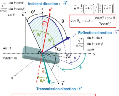
Figure 1 describes the detailed geometry of the propagation of the radiation across a rough sea surface in the configuration of a downward incident beam coming from the atmosphere and entering into the ocean layer.
Fig. 1. Geometry of the propagation of the light across a rough sea surface for the case of a downward incident beam coming from the atmosphere and entering into the ocean (air to sea). The directions of the incident beam, the reflection and the transmission of light are shown. In Fig. 1, the notations are as follows: θia is the incidence angle (i.e. half angle between the
incident and the reflection directions), θtw is the angle of refraction relative to the direction
perpendicular to the facet of the wave n
, θn is the zenith angle that corresponds to the direction perpendicular to the facet of wave, θt is the zenith angle of the transmission direction,
φ is the azimuth, s, v, and t are the vectors describing the coordinates of the incident, reflected and transmitted light respectively. m is the refractive index of the water.
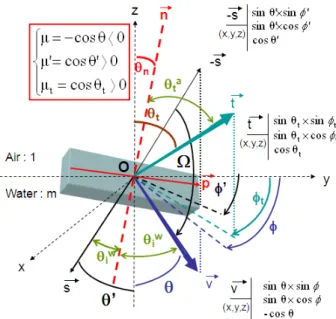
Figure 2 describes the detailed geometry of the propagation of the radiation across a rough sea surface in the configuration of an upward radiation exiting the ocean.
Fig. 2. Geometry of the propagation of the light across a rough sea surface for the case of an upward radiation exiting the ocean (sea to air). The directions of the incident beam, the reflection and the transmission of light are shown. The incident direction is given by the vector
s
−. In Fig. 2, the notations are as follows: θiw and θta are respectively the incidence angle and
the angle of refraction relative to the direction perpendicular to the facet of wave n. θn is the
zenith angle that corresponds to the direction perpendicular to the facet of wave. θ’ and φ' are respectively the zenith and azimuth angle of the incident beam relative to the vertical axis z. θ’
and φ' are the zenith and azimuth angle of the reflected beam. s, v, and t are the vectors
describing the coordinates of the incident, reflected and transmitted light respectively. m is the
refractive index of the water.
2.2.2 Modelling of the reflection matrix of the light scattered in the atmosphere onto the sea surface (reflection “air to air”)
The components of the incident Stokes vector (direct solar beam and diffuse light) that are reflected onto the sea toward the direction (μr, φr), for the first order of scattering in the
atmosphere (order 1) and the other orders (order n), are expressed as follows [Eq. (3)]:
( ) ( ) ( ) ( ) ( ) ( ) R 1 0 0 0 2 0 R n n 1 ' 0 ' 1 1
Order 1: L , , RAA , , , . exp / ,
4π. 1 Order n :L , , RAA , , ', ' L , ', ' . ' . ', 4π. r r r r r r r r r r E d d π ϕ μ τ μ ϕ μ ϕ μ ϕ τ μ μ τ μ ϕ μ ϕ μ ϕ τ μ ϕ μ ϕ μ ↑ ↑ ↓ − = = − = × × = × ×
(3) where:μ’ = –cosθ’ (0 < θ’ < π/2) is the cosine of the zenith angle of the downwelling incident
light direction,
φ’ is the azimuth angle of the incident light direction, μ0 is the cosine of the solar zenith angle,
φ0 is the azimuth angle of the solar incident direction,
μr = cos θ (0 < θ < π/2) is the cosine of the zenith angle of the upwelling reflected light,
φr is the azimuth angle of the reflected light direction,
(
)
RAA μ ϕ μ ϕr, , ', 'r is the “air-air” surface reflection matrix for an incident beam coming
from the direction (μ’, φ’) and reflected toward the direction (μr, φr),
(
)
(
(
)
)
(
)
R n R n R n R n I , , L , , Q , , U , , τ μ ϕ τ μ ϕ τ μ ϕ τ μ ϕ ↑ ↑ ↑ ↑ = is the reflected Stokes vector at the order of scattering n,
resulting from the reflection on the sea surface of the incident light at the order of scattering n-1, E 0 0 E =
is the solar irradiance at Top Of Atmosphere (TOA) coming from the direction
(μ0, φ0). As mentioned above, the convention that is used in both the OSOA and OSOAA
models is to consider a solar irradiance value E that is equal to π,
(
)
n 1
L↓− τ μ ϕ, ', ' is the incident Stokes vector at the order of scattering n-1 (which
corresponds to the diffuse incident light at the surface level).
In the presence of a rough sea surface, the surface reflection matrix “air to air”
(
)
RAA μ ϕ μ ϕr, , ', 'r , that is mentioned in Eq. (3), is determined by the Fresnel reflection matrix, noted RFAA, which should be weighted by the probability function, noted gR, of
encountering a wave facet given the geometrical configuration of the incident and the reflected directions [Eqs. (4) and (5)]. It should be highlighted that the weighting of RFAA by
gR was not performed in the previous OSOA code because the geometry of the specular
reflection is well determined in the case of a flat sea surface. As far as a rough surface is considered, the specular reflection remains valid for each wave slope. The solar reflected light toward any desired observation geometry is then calculated by taking into account for the statistics of wave slopes geometry by the weighting function gR (correlated to the wind
speed).
Since the Fresnel reflection matrix from a reference frame associated to the reflection plane is well known, the application of rotation matrices is required to take into account the transition to frames associated to the incident meridian plane and to the reflection meridian plane from the reflection plane [Eq. (6)].
(
)
R(
)
( )
AA( )
RAA , , ', ' g , , ', ' .RF ( ).a ' , r r r r i μ ϕ μ ϕ = μ ϕ μ ϕ × ℜ −χ θ ℜ χ (4) where:(
)
2 4 22 tan 1 , , ', ' exp , .cos n R r r n g μ ϕ μ ϕ θ σ θ σ = × − (5) σ2 is given by Eq. (2),χ’ is the rotation angle between the direction perpendicular to the incident meridian plane
and the direction perpendicular to the reflection plane,
-χ is the rotation angle between the direction perpendicular to the reflection plane and the
direction perpendicular to the reflection meridian plane,
( )
χ'ℜ is the rotation matrix that is expressed as follows [Eq. (6)]:
( )
' 10 cos 2 '0 sin 2 ' .0 0 sin 2 ' cos 2 ' χ χ χ χ χ ℜ = − (6)AA
RF ( )a i
θ is the Fresnel reflection matrix (air to air) for a reference frame associated to the reflection plane, where θιa is the incidence angle from the atmosphere relative to the vector
perpendicular to the wave facet as expressed within Fig. 1. The Fresnel reflection matrix is expressed as follows [Eqs. (7)–(10)]:
( )
11 12 AA 12 11 33 R ( ) R ( ) 0 RF R ( ) R ( ) 0 , 0 0 R ( ) a a i i a a a i i i a i θ θ θ θ θ θ = (7) where:(
) (
)
(
) (
)
2 2 11 r 2 2 12 r 33 r R ( ) 0.5 r ( ) r ( ) , R ( ) 0.5 r ( ) r ( ) , R ( ) r ( ) r ( ), a a a i i i a a a i i i a a a i i i θ θ θ θ θ θ θ θ θ = × + = × − = × (8) 2 2 2 2 2 2 m .cos - m -sin ( ) r ( ) , m .cos m -sin ( ) a a i i a i a a i i θ θ θ θ θ = + (9) 2 2 2 2 cos - m -sin ( ) r ( ) , cos m -sin ( ) a a i i a r i a a i i θ θ θ θ θ = + (10)2.2.3 Modelling of the transmission matrix of the light scattered in the atmosphere from the air to the sea medium
Similarly as for the reflection matrix [Eq. (3)], the transmission matrix of the direct solar beam and of the diffuse light through the sea surface toward the direction (μt, φt) is expressed
for the first order of scattering and any other order n as follows [Eq. (11)]:
( ) ( ) ( ) ( ) ( ) ( ) 0 T1 0 0 0 2 0 0 0 T n n 1 ' 0 ' 1 1
Order 1: L , , TAW , , , . . exp / , π. 1 Order n : L , , TAW , , ', ' .L , ' , ' . ' . ', π. t t t t t t t t t t E d d π ϕ μ τ μ ϕ μ ϕ μ ϕ τ μ μ τ μ ϕ μ ϕ μ ϕ τ μ ϕ μ ϕ μ ↓ − ↓ − ↓ + − = = − = × = ×
(11) where:μt = cos θt (0 < θt < π/2) is the cosine of the zenith angle of the downwelling transmitted
light,
φt is the azimuth angle of the transmitted light,
(
)
TAW μ ϕ μ ϕt, , ', 't is the transmission matrix from the air to the sea medium for an incident beam coming from the direction (μ’, φ’) that is transmitted toward the direction (μt,
φt),
(
)
0 Tn
L↓ − τ μ ϕ, ,t t is the Stokes vector at an order of scattering n, just beneath the sea surface (noted as the level 0-), resulting from the transmission through the sea surface of the incident light at the previous order of scattering (order n-1).
The transmission matrix TAW
(
μ ϕ μ ϕt, , ', 't)
from air to sea is expressed as follows [Eq.(
)
(
) ( )
( )
(
)
FLUX AW t T t 2 2 TAW μ , ,μ', ' g μ , ,μ', ' .TF ( ). ' .cos .cos , .cos cos a t t t i t w a t i w a t i m m ϕ ϕ ϕ ϕ χ θ χ θ θ θ θ = ×ℜ − ℜ × − (12) where:θia is the incidence angle from the atmosphere relative to the vector perpendicular to the
wave facet,
θtw is the refraction angle into the sea relative to the vector perpendicular to the wave facet
[Fig. 1],
χt’ is the rotation angle between the direction perpendicular to the incident meridian plane
and the direction perpendicular to the transmission plane,
-χt is the rotation angle between the direction perpendicular to the transmission plane and
the direction perpendicular to the transmission meridian plane,
m is the refractive index of seawater,
gT(μt, φt, μ’, φ’) is the probability function of encountering a wave facet for the incident
direction (μ’, φ’) and the transmission direction (μt, φt). Since there is a single configuration of
the reflected and transmitted light given the geometry of the incident light and of the wave facet, the probability function gT and gR are related as follows [Eq. (13)]:
(
)
(
)
T t R r
g μ , ,μ', 'ϕt ϕ =g μ , ,μ', ' .ϕr ϕ (13) The matrix TFFLUXAW ( )θia [Eq. (12)] is the Fresnel transmission matrix from the air to the
sea medium for a reference frame associated to the transmission plane. It is expressed as follows [Eqs. (14)-(17)]:
( )
11 12 FLUX AW 12 11 33 t ( ) t ( ) 0 m.cos TF t ( ) t ( ) 0 , cos 0 0 t ( ) a a i i w a t a a i a i i i a i θ θ θ θ θ θ θ θ = × (14) where:(
) (
)
(
) (
)
2 2 11 r 2 2 12 r 33 r t ( ) 0.5 t ( ) t ( ) , t ( ) 0.5 t ( ) t ( ) , t ( ) t ( ) t ( ), a a a i i i a a a i i i a a a i i i θ θ θ θ θ θ θ θ θ = × + = × − = × (15)(
)
1 t ( ) 1 r ( ) , m a a i i θ = × + θ (16) t ( ) 1 r ( ).a a r θi = + r θi (17)2.2.4 Modelling of the reflection matrix of the upward light scattered within the ocean that is reflected onto the sea surface (“sea to sea”)
The upwelling Stokes vector within the ocean only consists of diffuse light since the direct solar beam is a downward illumination. The reflection matrix that applies for the upwelling Stokes vector within the ocean that is reflected onto the sea surface toward the direction (μr,
(
)
(
)
2 1(
)
(
)
R n n 1 ' 0 ' 0 1 L 0-, , RWW , , ', ' .L 0-, ', ' . '. ', 4π. sea sea r r r r r d d π ϕ μ μ ϕ μ ϕ μ ϕ μ ϕ μ ϕ μ ↓ ↑ − = = = × −
(18) where:μ’ is the cosine of the zenith angle of the upwelling incident light direction,
φ’ is the azimuth angle of the incident light direction,
μr is the cosine of the zenith angle of the downwelling reflected light,
φr is the azimuth angle of the reflected light,
(
)
RWW μ ϕ μ ϕr, , ', 'r is the surface reflection matrix from “sea to sea” for an incident beam coming from the direction (μ’, φ’) that is reflected toward the direction (μr, φr),
(
)
R n
L↓sea 0-, ,μ ϕ is the Stokes vector at an order of scattering n, resulting from the reflection onto the sea surface (level 0- just beneath the sea surface) of the upwelling incident light at order of scattering n-1,
(
)
n 1
L↑sea− 0-, ', 'μ ϕ is the incident Stokes vector at an order of scattering n-1 (diffuse
upwelling light at sea surface at level 0-).
The surface reflection matrix “sea to sea” RWW
(
μ ϕ μ ϕr, , ', 'r)
is calculated from the Fresnel reflection matrix RFWW which should be weighted by the probability function gR ofencountering a wave facet [Eq. (19)]. The rotation matrices that are used to bring the frame associated to the incident meridian plane from the frame associated to the reflection meridian plane via the reflection plane should be accounted for as well in the calculation of
(
)
RWW μ ϕ μ ϕr, , ', 'r [Eq. (19)].(
)
(
)
(
)
WW( )
RWW , , ', ' , , ', ' .RF ( w). ' , R r r w i w g μ ϕ μ ϕ = μ ϕ μ ϕ × ℜ −χ θ ℜ χ (19) where:gR has been defined at Eq. (5),
χw’ is the rotation angle between the direction perpendicular to the incident meridian plane
and the direction perpendicular to the reflection plane,
-χw is the rotation angle between the direction perpendicular to the reflection plane and the
direction perpendicular to the reflection meridian plane,
( )
χ'ℜ is the rotation matrix defined by Eq. (6).
The matrix RFWW(θiw) [Eq. (19)] is the Fresnel reflection matrix (“sea to sea”) for a
reference frame associated to the reflection plane. RFWW(θiw) is expressed as follows [Eqs.
(20)-(23)]: 11 12 WW 12 11 33 R ( ) R ( ) 0 RF ( ) R ( ) R ( ) 0 , 0 0 R ( ) w w i i w w w i i i w i θ θ θ θ θ θ = (20) where:
θiw is the incidence angle from the sea water relative to the vector perpendicular to the
(
) (
)
(
) (
)
2 2 11 r 2 2 12 r 33 r R ( ) 0.5 r ( ) r ( ) , R ( ) 0.5 r ( ) r ( ) , R ( ) r ( ) r ( ), w w w i i i w w w i i i w w w i i i θ θ θ θ θ θ θ θ θ = × + = × − = × (21)( )
( )
2 2 2 2 cos m 1-m .sin r ( ) , cos m 1-m .sin w w i i w i w w i i θ θ θ θ θ − × = + × (22)( )
( )
2 2 2 2 m.cos 1-m .sin r ( ) . m.cos 1-m .sin w w i i w r i w w i i θ θ θ θ θ − = + (23)Note that for the case of a total reflection due to the critical angle in the water θlimw , the
terms of the Fresnel reflection matrix are defined as follows [Eq. (24)]:
11 lim 12 lim 33 lim R ( ) 1, R ( ) 0, R ( ) 1. w w i w w i w w i θ θ θ θ θ θ > = > = > = (24)
2.2.5 Modelling of the transmission matrix of the upward light scattered within the ocean from “sea to air”
The transmission through the sea surface of the upward Stokes vector, toward the direction (μt, φt), is expressed as follows [Eq. (25)]:
(
)
2 1(
)
(
)
Tn n 1 ' 0 ' 0 1 L 0 , , TWA , , ', ' .L 0-, ', ' . '. ', π. sea sea t t t t t d d π ϕ μ μ ϕ μ ϕ μ ϕ μ ϕ μ ϕ μ ↑ ↑ − = = + = ×
(25) where:μt = cos θt (0 < θt < π/2) is the cosine of the zenith angle of the upwelling transmitted light,
φt is the azimuth angle of the transmitted light direction,
(
)
TWA μ ϕ μ ϕt, , ', 't is the surface transmission matrix from the sea to the air for an
incident beam coming from the direction (μ’, φ’) that is transmitted toward the direction (μt,
φt),
(
)
Tn
L sea 0 , ,μ ϕt t
↑
+ is the Stokes vector at order of scattering n, just above the sea surface (noted level 0 + ), resulting from the transmission through the surface of the incident Stokes vector at the order of scattering n-1.
The surface transmission matrix “sea to air” TWA
(
μ ϕ μ ϕt, , ', 't)
is expressed as follows [Eq. (26)]:(
)
(
) (
)
( )
(
)
(
)
FLUX WA t T t 2 TWA μ , ,μ', ' g μ , ,μ', ' .TF . ' cos .cos , .cos cos w t t wt i wt a w t i w a i t m ϕ ϕ ϕ ϕ χ θ χ θ θ θ θ = ×ℜ − ℜ × − (26) where:θiw is the incidence angle from the sea relative to the vector perpendicular to the facet of
the wave [Fig. 2],
θta is the refraction angle into the air relative to the vector perpendicular to the facet of the
wave,
χwt’ is the rotation angle between the direction perpendicular to the incident meridian plane
and the direction perpendicular to the transmission plane,
-χwt is the rotation angle between the direction perpendicular to the transmission plane and
the direction perpendicular to the transmission meridian plane,
gT(μt, φt, μ’, φ’) has been defined at Eq. (13).
( )
FLUX WA
TF w
i
θ is the Fresnel transmission matrix from sea to air for a reference frame associated to the transmission plane. It is expressed as follows [Eqs. (27)–(30)].
( )
11 12 FLUX WA 12 11 33 t ( ) t ( ) 0 cos TF t ( ) t ( ) 0 , m.cos 0 0 t ( ) w w i i a w t w w i w i i i w i θ θ θ θ θ θ θ θ = × (27) where:(
) (
)
(
) (
)
2 2 11 r 2 2 12 r 33 r t ( ) 0.5 t ( ) t ( ) , t ( ) 0.5 t ( ) t ( ) , t ( ) t ( ) t ( ), w w w i i i w w w i i i w w w i i i θ θ θ θ θ θ θ θ θ = × + = × − = × (28)(
)
t ( w) m 1 r ( w) , i i θ = × + θ (29) t ( w) 1 r ( w). r θi = + r θi (30)3. Validation and performance of the OSOAA model
Since the flat sea surface OSOA model has already been validated in details by Chami et al. [11], the validation procedure of the OSOAA model is focused on the validation of the implementation of the rough sea surface, bearing in mind that it was first verified that both OSOA and OSOAA models provide exactly similar results for a flat sea surface (i.e., σ2 = 0 in
[Eq. (2)]). Therefore, specific cases of simulations are defined to test and to verify the correct implementation of the rough sea surface. The results are then compared with those obtained by the extended General Adding Program (eGAP) code. This code is originally based on the work done by De Haan et al. [31] for polarized light scattered by isolated atmospheres, and was extended by Chowdhary [32] to include polarized light scattering by ocean systems [see also 17,44]. The eGAP model solves the radiative transfer model using the adding/doubling method. The similarities between eGAP and OSOAA are as follows: (i) they both use the Stokes vector formalism; (ii) they both expand the Stokes vector into a Fourier series; (iii) the same set of Gaussian quadrature angles is used for the intercomparison; (iv) they both use the geometrical optics approach to obtain the sea surface matrices from the Cox and Munk (1954) surface slope model. Hence, eGAP and OSOAA also share many numerical features which means that the successful cross-comparison made here verifies that the OSOAA model is coded properly and that the solution method used by OSOAA to solve the radiative transfer equation and to model the roughened sea surface in the atmosphere-ocean system is robust.
In addition to the intercomparison exercise, the conservation of the radiant fluxes along the atmosphere-ocean system in the presence of a rough sea surface is verified as well to check self-consistency of the OSOAA model.
3.1 Intercomparison between the OSOAA and eGAP models for the validation of the implementation of the rough sea surface
The Stokes parameters (I,Q,U) calculated by OSOAA model are compared with the results obtained by the eGAP code to validate the correct implementation of the diffuse and solar direct light reflection/transmission through the air/sea interface. The simulations take into account all the scattering processes that occur in the atmosphere-ocean system. They also include all the interactions between the air and the sea interface for a rough sea surface (i.e. for a wind speed value different from zero). The comparisons that are discussed here are carried out for the level just above the sea surface (level 0 + ).
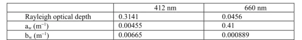
The conditions of the simulations are as follows. The calculations are performed at the wavelengths 412 nm and 660 nm which are representative of cases showing a high and a low number of scattering events in the atmosphere-ocean system including close to the air-sea interface. The solar zenith angle value is 30°, the number of Gaussian quadrature angles for the atmosphere is 40, the atmospheric scattering is only due to molecules (i.e., purely Rayleigh atmosphere with no aerosols), the oceanic constituents only consist of water molecules (i.e. no hydrosols). The reduced 3x3 Mueller scattering matrices of Rayleigh and water molecules used here are similar to those which are described by Mishchenko et al. [33] and by Adams and Kattawar [34] respectively. The optical properties of the air and water molecules used for the simulations are reported in Table 1. The factor of molecular depolarization in the air and in the sea is zero. The sea bottom depth is 1000 m, with a sea bottom albedo value of 0. The wind speed value W is set at 7 m s−1 and the wave distribution
is determined using the Cox and Munk model [30]. The output of the simulations is the angular distribution of the Stokes parameters I, Q and U normalized to an extraterrestrial irradiance value of π. Note that the convention used in OSOAA model (and in the forthcoming figures) to define azimuth angles is that a relative azimuth angle of 180° corresponds to the plane that contains the sun in the solar plane (i.e. the vertical half-plane containing the backscattering direction) while a relative azimuth angle of 0° corresponds to the half-plane that contains the specular reflection in anti-solar half-plane (i.e. the vertical half plane containing the sunglint of a flat ocean surface).
Table 1. Values of the optical properties of the air and seawater molecules used for the validation of OSOAA model. The absorption and scattering coefficients of pure seawater,
noted aw and bw respectively, are also reported (in m−1).
412 nm 660 nm
Rayleigh optical depth 0.3141 0.0456
aw (m−1) 0.00455 0.41
bw (m−1) 0.00665 0.000889
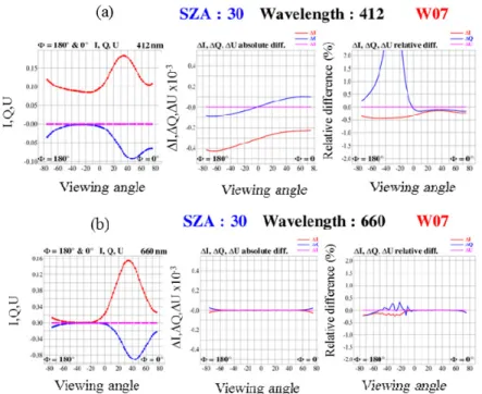
Figure 3 shows the results of the comparison of the upward Stokes parameters (I, Q, U) that are calculated just above the sea surface (level 0 + ) by the OSOAA and eGAP radiative transfer codes.
Fig. 3. Comparisons of the Stokes parameters I, Q and U normalized to an extraterrestrial irradiance value of π as a function of the viewing angle between the eGAP and OSOAA models at the sea surface level (level 0 + ): (a) at 412 (top panel) and (b) at 660 nm (lower panel) for the conditions of simulations outlined in section 3.1 (solar zenith angle SZA value of 30°, wind speed value of 7 m s−1 (W07)). In the left column, eGAP calculations are shown as
solid lines; OSOAA outputs are shown as dotted lines. The absolute differences (middle column) between the eGAP and OSOAA Stokes parameters are noted ΔI = IeGAP-IOSOAA, ΔQ =
QeGAP-QOSOAA and ΔU = UeGAP-UOSOAA. The relative differences (right column), which are defined as ΔI/IeGAP, ΔQ/QeGAP, ΔU/UeGAP, are expressed in percents.
A very nice agreement is obtained between both radiative transfer models. At 412 nm, where the interactions between the scattered light within the atmospheric or oceanic layers and the sea surface are the most important, the absolute differences are lower than 0.4 × 10⁻³
for the Stokes parameter I (i.e. radiance) and lower than 0.1 × 10⁻³ for Q and U. The relative
differences are not greater than 0.8% except for the parameters Q and U in the particular case where viewing angles corresponds to a degree of polarization very close to zero. For this specific latter geometry, the relative difference is meaningless since the division by a number close to zero leads to artificial high relative differences values. At 660 nm, where the number of scattering events is much lower than at 412 nm, the absolute differences are lower than 0.02 × 10⁻³ for all Stokes parameters.
Similar satisfactory agreements between the eGAP and OSOAA models were obtained for other conditions of simulations, such as other solar zenith angle (i.e. 60°), other azimuth values (i.e. φ = 90°), other wind speed values (i.e. 5 m s−1 and 10 m s−1) and other level of
observation (i.e. TOA). Note that the comparisons between the eGAP and OSOAA models for results obtained at TOA level showed relative differences values less than 0.2%, which are even lower than those observed at the sea surface level 0 + [Fig. 3] due to the fact that the amplitude of the upward radiation at TOA has undergone fewer interactions with the ocean surface-body system than at the level 0 + . The overall inter-comparisons performed between OSOAA and eGAP models confirm the good implementation of the rough sea surface within OSOAA model.
3.2 Conservation of energy within OSOAA model
An important verification that needs to be performed to make sure that the implementation of the rough sea surface within the radiative transfer code does not induce any loss of photons relies on checking that the energy is conserved when the radiation propagates across the sea surface. In other words, there should not be any loss of photons between the atmosphere and the ocean due to the introduction of a rough sea surface. A simple way to carry out this verification is to compare the downward plane irradiance (defined as the integral of the radiance over the lower hemisphere), hereafter referred to as Ed, with the upward irradiance
(defined as the integral of the radiance over the upper hemisphere), hereafter referred to as Eu,
at the sea surface level (i.e. level 0 + and level 0-). For that purpose, simulations were carried out for the specific following conditions. The solar zenith angle value is 30°, the extraterrestrial solar irradiance value is equal to π, both the atmosphere and ocean are supposed to be completely transparent (i.e., no scattering or absorption processes in each layer), the sea bottom albedo is zero, the wind speed value is 7 m s−1. Since there are no
scattering processes occurring in the atmosphere and ocean layers here, the results of the calculations are independent of the wavelength. For these specific simulations conditions (transparent atmosphere and ocean): the downwelling plane irradiance just above the sea surface, Ed(0 + ), only consists of the direct solar beam; the downwelling irradiance just
beneath the surface, Ed(0-), only consists of the direct solar beam that is transmitted into the
ocean, the upwelling irradiance just above the sea surface, Eu(0 + ), only consists of the
reflection of the direct solar beam onto the sea surface. Therefore, the conservation of energy implies that the incident flux should be equal to the sum of the transmitted flux and the reflected flux. The conservation of energy could thus be expressed as follows [Eq. (31)]:
(0 ) (0 ) (0 ) (0 ),
d d u u
E + =E − +E + +E − (31) where Eu(0-), which is the upwelling irradiance just below the sea surface, is equal to zero
here since there is no scattering or sources in the ocean component. The results clearly show that the conservation of energy within the OSOAA model is verified by less than 0.01%, which is highly satisfactory (Table 2). Note that a good consistency (less than 1%) was obtained as well at other solar zenith angle (e.g., 60°). Therefore, the implementation of the rough sea surface does not induce any significant loss of photons thus confirming the self-consistency of the OSOAA model. Some loss of photons could be expected (i.e., the relative difference in Table 2 is not exactly 0%) because the sea surface model used in OSOAA does not account for photon paths in which reflection from the side of a wave directly leads to a further interaction with another wave surface as it could be done when a full 3D structure is used to model the sea surface [26]. The consideration for multiple interactions at the sea surface as a 3D structure modelling could provide is to ensure an exact conservation of energy within the model as recently highlighted by Mobley [26]. However, the satisfactory results of Table 2 show that neglecting the photons interacting from one wave to another within OSOAA model remains a second-order effect which should not induce large errors in the calculations of the Stokes vector across the sea surface.
Table 2. Results showing the conservation of energy within OSOAA model based on Eq. (31). Ed(0 + ) is the downwelling plane irradiance just above the sea surface; Ed(0-) is the downwelling irradiance just beneath the surface, Eu(0 + ) is the upwelling irradiance just
above the sea surface. The simulations are carried out using OSOAA model with a transparent atmosphere, a transparent ocean, and a solar zenith angle of 30 degrees (see
section 3.2 for details). Since the extraterrestrial solar irradiance value is π, the irradiances values are dimensionless. The relative difference between Ed(0 + ) and the
sum (Ed(0-) + Eu(0 + )) is also reported (in %).
Ed(0 + ) Ed(0-) Eu(0 + ) Ed(0-) + Eu(0 + ) Relative difference between column 1 and 4 (in %)
3.3 Performance and improved capabilities of simulation of the OSOAA model
In addition to the consideration of the rough sea surface, the OSOAA model has many other improvements relatively to the initial OSOA model from which it is based [11]. The number and the complexity of available aerosol and hydrosol models are more realistic than for OSOA model thus making the inputs of the simulations more close to real-world conditions. As an example, aerosols models could be defined either based on well-known models taken from the literature such as the Shettle and Fenn model [35] and the World Meteorological Organization (WMO) [36] models, or by the user himself using various type of size distributions (e.g., power law, mix of log normal size distributions for the fine and coarse modes). The hydrosol models can also be defined using a mix of size distributions (power law and log normal distributions) that is helpful to emphasize special modes of hydrosol size that can happen in natural waters, during phytoplankton blooms conditions for example.
Another originality of the OSOAA model is its capability to use measurements of the scattering function (for intensity) or scattering matrix (for polarization) of aerosols and hydrosols as input of the computations. Such capability is of primary importance to correctly model the marine reflectance using measurements of the volume scattering function of hydrosols. That should be more available in the near future due to the recent development of many volume scattering meters instruments [37–42].
It should also be highlighted that an interesting advantage of the OSOAA model is that it provides outputs of the radiance and degree of polarization at all levels (altitude or depth) within the atmosphere and the ocean layers. The initial OSOA model only provided outputs at the sea surface or at the top of atmosphere level. The advanced OSOAA model could thus be used for applications like underwater vision which requires knowledge of the radiance at various depths within the ocean.
Finally, the OSOAA radiative transfer model has been developed to ensure an operational use by any users for the computations of the Stokes vector (radiance and degree of polarization) throughout the atmosphere-ocean system in the presence of a rough sea surface. For that purpose, a graphical user interface (GUI) has been developed to perform runs of simulations in a user-friendly environment. Note also that the model could be launched using a command line file which permits launching many runs of computations, which is highly useful for generating Look Up Tables.
The numerical resolution of the radiative transfer equation by OSOAA model has been optimized to ensure fast computations which include all the multiple scattering processes in the atmosphere and ocean layers. As an example, the duration of the computation of the Stokes parameters for a purely Rayleigh atmosphere (i.e. no aerosols) and only pure seawater (i.e. no hydrosols) at 443 nm for an ocean depth of 1000m is 2.5 seconds when the simulation is performed on a PC Linux Redhat 5 64bits system (processor XW4600 CORE 2 DUI E8500). Such a satisfactory computation speed associated to the very good validation results of OSOAA model presented in section 3.1 where OSOAA model was shown to be consistent with eGAP model within 0.8% thus confirm the good performance and accuracy of the OSOAA code.
4. Application of the OSOAA model to the characterization of the directionality of the water leaving reflectance for a rough interface
Knowledge of the angular dependence of the water leaving reflectance, which is defined as the ratio between the water leaving radiance and the downwelling irradiance just above the sea surface (level 0 + ), is of great interest for correctly modelling the radiation that is received at the top of atmosphere by multi-angular satellite sensors like the POLDER sensor (Centre National d’Etudes Spatiales) [43] or the forthcoming “Multi-Viewing, Multi-Channel, Multi-Polarization Imaging Mission (3MI)” mission (European Space Agency/Eumetsat). The consideration of the multi-angular properties of the light exiting the ocean in the inverse
algorithms that are applied to satellite images should improve as well the detection of the aerosols. As an example, it was previously shown that the directional effects of the water-leaving reflectance at short visible wavelengths (lower than 550 nm) on the signal modeled at the top of the atmosphere needs to be accounted for to accurately retrieve the aerosol properties from multi-angular observations [44–46]. However, most of the inverse algorithms that are currently used to determine the aerosol properties from multidirectional radiation received at the top of atmosphere either assume a Lambertian water leaving reflectance (i.e. the water leaving reflectance is independent of the geometry of observation) [47–49] or use a two-components ocean surface directional reflectance model which takes into the directional effects of sunglint and whitecaps [50] regardless of the directional effects induced by the hydrosols themselves.
The angular dependence of the oceanic surface has been previously studied in the literature by oceanographers [51–54]. However, the formalism that is used by oceanographers to quantify the directionality of the water leaving reflectance relies on an analytical linearization of the radiative transfer equation proposed by Morel and Prieur [55]. The linearization consists in establishing a relationship between the water leaving reflectance and the optical properties of the hydrosols (i.e. absorption and backscattering coefficients) through a factor, so-called “f/Q” factor, which accounts for the directionality of the radiation. The representation of the directional effects induced by the water leaving reflectance using the simple “f/Q” factor is not really appropriate if one aims at retrieving the aerosol optical properties from satellite multi-angular data over the ocean. This is because knowledge of the remote sensing directional reflectance is required as inputs of inverse algorithms in this latter case [56]. Here, simulations are carried out using the OSOAA model to characterize the directional variations of the water leaving reflectance (at the level 0 + ) induced by the hydrosols. The influence of the wind speed on these directional variations is also investigated.
4.1 Conditions of simulations
The computations are performed for two oceanic conditions: (i) a phytoplankton dominated water type (i.e. no mineral-like particles), and (ii) a mineral-like particles dominated water type (i.e. no phytoplankton particles). The full conditions of simulations are as follows. The solar zenith angle value is set to 30°, the aerosol model is the Shettle and Fenn [35] maritime model with a relative humidity of 98% (model M98), the aerosol optical depth at 550 nm is 0.2, the scattering matrix (phase function and degree of polarization) of phytoplankton particles is modelled using Mie theory with a refractive index of 1.05 and a Junge power law size distribution having an exponent value of 4, which is the average exponent value within the range of exponent values typically found in the ocean. The chlorophyll a concentration is 1 mg m−3. The scattering matrix of mineral-like particles is modelled using Mie theory with a
refractive index of 1.15 and a Junge power law size distribution having an exponent value of 4. The concentration of the sediments is 5 mg.ℓ−1. The scattering and absorption coefficients
of the hydrosols are obtained using the same bio-optical models as those used in the initial OSOA radiative transfer code (see [11] for details). The sea bottom albedo is zero (black bottom). The computations are performed at 443 nm, which is an ocean color wavelength where the number of scattering events is high, for various wind speed values, namely 2 m s−1,
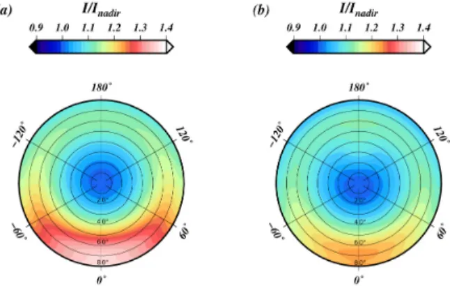
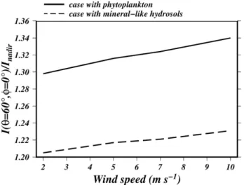
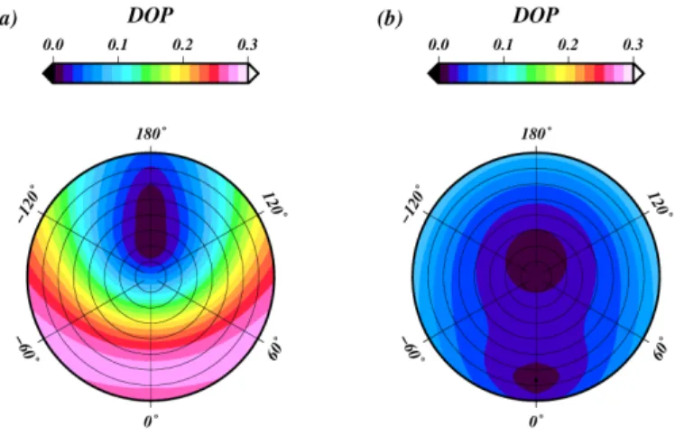
5 m s−1, 7 m s−1 and 10 m s−1. The outputs of the simulation consist of polar diagrams
representing the ratio between the water leaving reflectance at a given geometry (azimuth and viewing angles), hereafter noted as I, and the water leaving reflectance for the nadir direction (i.e. the viewing angle is 0°), hereafter noted as Inadir. Such a ratio is relevant since it directly
quantifies the directional effects of the ocean and the difference with the Lambertian assumption. It should be highlighted that the value of the ratio I/Inadir is supposed to be 1 for a
Lambertian surface since the radiance I is independent of the geometry of observation in Lambertian conditions. To make sure that the water leaving reflectance only consists of the contribution of the signal exiting the ocean, the computations were performed in two steps.